Tackling Uncertainty: Forecasting the Energy Consumption and Demand of an Electric Arc Furnace with Limited Knowledge on Process Parameters

Abstract

The iron and steel industry significantly contributes to global energy use and greenhouse gas emissions. The rising deployment of volatile renewables and the resultant need for flexibility, coupled with specific challenges in electric steelmaking (e.g., operation optimization, optimized power purchasing, effective grid capacity monitoring), require accurate energy consumption and demand forecasts for electric steel mills to align with the energy transition. This study investigates diverse approaches to forecast the energy consumption and demand of an electric arc furnace—one of the largest consumers on the grid—considering various forecast horizons and objectives with limited knowledge on process parameters. The results are evaluated for accuracy, robustness, and costs. Two grid connection capacity monitoring approaches—a one-step and a multi-step Long Short-Term Memory neural network—are assessed for intra-hour energy demand forecasts. The one-step approach effectively models energy demand, while the multi-step approach encounters challenges in representing different operational phases of the furnace. By employing a combined statistic–stochastic model integrating a Seasonal Auto-Regressive Moving Average model and Markov chains, the study extends the forecast horizon for optimized day-ahead electricity procurement. However, the accuracy decreases as the forecast horizon lengthens. Nevertheless, the day-ahead forecast provides substantial benefits, including reduced energy balancing needs and potential cost savings.

1. Introduction

Industry accounts for approximately one-third of global energy consumption and is expected to maintain this share in the future [1]. Modelling and forecasting industrial energy use remain challenging yet essential tasks. Furthermore, the increasing deployment of volatile renewable energy sources is expected to pose challenges to the energy system, leading to higher levels of uncertainty that affect future electricity (spot) market prices and increase the demand for flexibility [2], including individual energy-intensive industrial units participating in energy or capacity markets.

The iron and steel industry is a major industrial contributor to global energy consumption and greenhouse gas emissions (7% in 2021) [3]. In 2018, 1.8 million tonnes of crude steel were produced, mainly through the blast furnace and basic oxygen furnace (BF-BOF) route (71%). The alternative electric arc furnace (EAF) route is a low-carbon alternative, emitting only 0.46 t CO₂ per ton of crude steel, significantly less than the 2.20 t CO₂ emitted by the BF-BOF route [4]. The primary reason for the difference lies in the input materials used: the BF-BOF route uses iron ore, whereas the EAF route uses steel scrap. As such, electric steel mills present an opportunity for the decarbonization and electrification of the iron and steel industry; with a production share of 24% in 2018, their use is expected to increase in the coming decades [3]. Nonetheless, the EAF route faces challenges, including power quality issues due to high power peaks and its batch-wise operation [4]. Despite these challenges, expanded deployment of renewables could reinforce the use of the EAF route. Since renewables like wind and solar are highly volatile, a reinforced employment requires accurate knowledge of the EAF process’ energy usage for various forecast horizons.

As electric steel mills are among the largest (electricity) consumers in the grids, energy consumption and demand forecasting can contribute to a secure grid operation [5]. Additionally, knowledge about temporal resolved future energy usage assists industrial sites in optimizing energy management, improving energy procurement strategies and avoiding costs associated with exceeding the maximum contracted grid connection capacity without affecting productivity. This knowledge also enables implementation of demand side management measures [6]. The stochastic operational behaviour, complexity, and limited insight into future process parameters of the upcoming batches make EAFs particularly challenging in terms of energy consumption and demand forecasts.

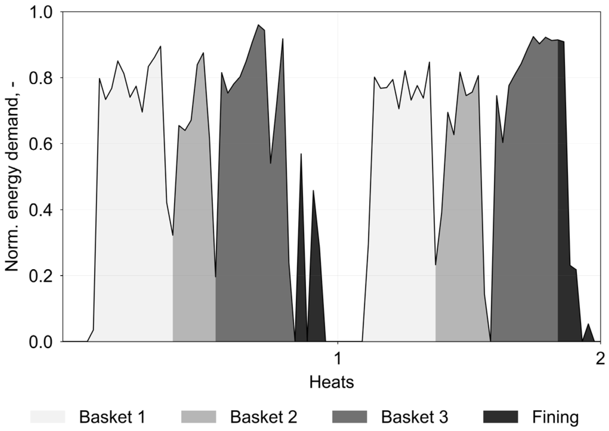
1.1. The EAF Process

An EAF is a vessel-like production unit utilized for melting steel scrap to produce various steel types. The EAF examined in this study accounts for app. 60% of the average energy consumption in the electric steel mill and exclusively produces reinforcing steel. This specific furnace is equipped with three graphite alternative current (AC) electrodes (85% of energy usage) and with three additional gas burners (15% of energy usage) to ensure better temperature distribution within the vessel and to enhance melting efficiency. As the initial unit in the process chain, its discontinuous operation mode sets the pace for all other downstream processes. Each operational cycle, referred to as a “heat”, encompasses multiple phases. It starts with a preparation phase, followed by charging and melting of typically three baskets of steel scrap. Scrap selection for the three baskets occurs at the onset of the heat or, for baskets 2 and 3, while the heat has already begun. Subsequent to the melting phases, the heat progresses to the fining phase. During this phase, pulverized coal and other additives are added to create foam slag. The purpose of foam slag is to absorb unwanted chemicals and remove them from the steel melt. In the final tapping phase, the foam slag is removed first, before the crude steel is poured into a preheated ladle, a refractory-lined container used for transporting the liquid crude steel to the subsequent process unit. Generally, little to no energy is required during the preparation and tapping phases. The entire duration required to complete a heat is referred to as tap-to-tap time. Figure 1 illustrates a representative energy demand curve of the examined EAF, delineating the various operational phases for two heats. Additionally,

Table 1. Average scrap mass, duration, and energy consumption of different operational EAF phases of the investigated EAF (normalized, in %).

	Scrap Mass [%]	Duration [%]	Heat-Based Energy Consumption [%]
Preparation	-	5.2	0.2
Basket 1	47.4	29.0	31.6
Basket 2	24.1	16.2	19.6
Basket 3	28.5	18.2	25.7
Fining	-	25.2	20.8
Tapping	-	6.2	2.1

provides specific details of average scrap masses, phase durations, and energy consumption shares for different operational phases of the examined EAF. The data for Figure 1 and Table 1 were provided by the EAF operator. Due to constraints in publishing the actual values of the examined EAF and confidentiality issues, all data and results in this study are presented in a normalized form.

Basket 1 exhibits the largest mass of inserted scrap (47.4%) and accounts for the highest proportion of energy consumption (31.6%). Basket 2, on the other hand, generally has the smallest scrap mass (24.1%). A significant share of the energy consumption is attributed to the fining phase (20.8%), during which metallurgical properties are adjusted.

The operational behaviour of the EAF is characterized by stochastic variability, primarily because melting steel scrap necessitates varying amounts of energy due to fluctuations in chemical composition [7]. Depending on the desired steel quality, specific scrap qualities are utilized. However, for reinforcing steel, minor scrap qualities suffice. The classification of scrap quality is based on the European Steel Scrap Specification [8]. This list specifies, beneath permissible bulk density, debris content and maximum dimensions of the scrap, that is, the target maximum concentrations of the chemical elements. The values specified for the analyses correspond to the practical empirical values of the various countries of the European Union. Therefore, the scrap qualities are in fact known. The main scrap qualities used in the investigated EAF are E1 (app. 35%) and E3 (app. 35%). The rest is made up of E3/E1 (app. 20%), and in extracts of E8, E40, and EHRM.

Table 2. Characteristics of utilized scrap qualities per European Steel Scrap Specification [8] (n.d. stands for not defined).

Category	Specification	Dimensions	Density	Steriles	Aimed Analytical Contents (Residuals) in %
					Cu	Sn	Cr, Ni, Mo
Old Scrap	E1	Thickness < 6 mm <1.5 × 0.5 × 0.5 m	≥0.5	<1.5%	≤0.400	≤0.020	Σ ≤ 0.300
Old Scrap	E3	Thickness ≥ 6 mm <1.5 × 0.5 × 0.5 m	≥0.6	≤1%	≤0.250	≤0.010	Σ ≤ 0.250
New Scrap	E8	Thickness < 3 mm <1.5 × 0.5 × 0.5 m	≥0.4	<0.3%	Σ ≤ 0.300	Σ ≤ 0.300	Σ ≤ 0.300
Shredded	E40	n.d.	>0.9	<0.4%	Σ ≤ 0.250	Σ ≤ 0.020	n.d.
High Residual Scrap	EHRM	max. 1.5 × 0.5 × 0.5 m	≥0.6	<0.7%	≤0.400	≤0.030	Σ ≤ 1.0

shows the specification of the main scrap qualities used. However, within a scrap class, the permissive range of chemical element concentrations is broad and it is still not guaranteed that the scrap fulfils the properties of the assigned scrap class.

Although fundamental EAF mechanisms have been extensively studied, they remain poorly understood due to extreme conditions and complexity. The energy dynamics within the vessel are influenced by various factors, such as scrap quality or bulk density, and lead to a heterogeneous temperature distribution. The nonlinear nature of the process, concerning power losses, electrode covering, or unexpected downstream events, must be taken into account [9]. Furthermore, despite the increased levels of automation in the EAF process, certain tasks, such as the sampling during the melting process, operation during the fining phase due to optical evaluation of the foam slag, manipulation while tapping, the selection and insertion of scrap, changing electrodes, or the overall high level of control, still heavily rely on the experience and decision making of the operating crew and can influence the progress of a heat significantly.

1.2. Forecast Modelling

Efforts to optimize future outcomes have given rise to forecast modelling, providing decision makers with necessary information to take appropriate actions [10]. In recent decades, various methods and approaches have evolved across scientific fields. According to the literature, there is no standardized classification of forecast approaches. In this study, we propose the following distinctions for energy forecast modelling (Figure 2):

Firstly, we categorize forecast models based on available information. Therefore, we focus on the input side of the model: “perfect knowledge” refers to seamless knowledge of future input parameters, system states, or production plans (known or deterministic) within the forecasting horizon. Forecasts based on specified scenarios also count in this category. In contrast, non-perfect knowledge models lack information about future input parameters (unknown or stochastic) and rely on observations from the past or historic data distributions. It has to be acknowledged that working with non-perfect knowledge is inextricably linked to uncertainties.

Secondly, we classify methodological approaches to address forecasting problems and distinguish between physics- or mathematics-based, statistics-based and machine learning. Physics- and mathematics-based approaches include thermodynamic laws and basic laws of physics and chemistry. It can be stated that different methods are suitable for forecasting different types of curves and processes [11]. Nonetheless, no concrete guidelines exist on how to forecast a certain variable regarding its curve characteristic and information about future states. The quality and applicability of a forecast still heavily depend on the set of skills and experience of the person who builds the model [12].

The forecast horizon is another important aspect of forecast modelling, describing the length of time in the future for which forecasts are to be prepared. Traditional terms like “short”, “mid”, and “long” are often used, but these terms are vague and lack uniformity. In the research field of photovoltaics, more precise terms such as “day-ahead”, “intra-day”, or “intra-hour” offer a higher level of precision [10] (Figure 3). These terms are better suited for forecasts related to electricity consumption and purchasing, as they reflect the market behaviour. The temporal resolution of a forecast links closely with the forecasting horizon, representing the density of forecasted data points within it. This resolution can range from milliseconds to several years, depending on the specific problem.

1.3. Energy Forecast Modelling of EAFs

Significant research has focused on modelling the EAF process and determining its energy consumption. As stated in Section 1.1, the stochastic nature of an EAF process makes that challenging and various approaches are investigated through different attempts:

One of the existing physics-based models is the work from Çamdalı and Tunç (2002) [13], investigating the influence of different process parameters on electric energy consumption. Similarly, Logar et al. (2011) [14] established a mathematical process model to describe the scrap-melting process for control design purposes and optimized energy use.

The review from Carlsson et al. (2019) [9] describes various statistics-based EAF models, including approaches like regular (multivariate) linear regression and combined with partial least squares regression. Dianmin et al. (2004) [15] investigated another type of linear regression using the nonnegative least squares method, including a random approximated greedy search (RAGS) for feature selection and information about maintenance periods and production plans to determine daily EAF energy consumption.

Machine learning approaches have recently gained popularity in EAF energy consumption modelling. Andonovski and Tomažič (2022) [16] used nine input variables and four operational phases to simulate the heat-wise energy consumption, comparing approaches like Support Vector Machines, k-nearest Neighbour, or Gaussian processes with Fuzzy Logic. Carlsson et al. (2019) [9] explored Artificial neural networks, Deep neural networks, and Random Forest methods for determining EAF energy consumption. Kovačič et al. (2019) [17] simulated heat-wise EAF energy consumption with genetic programming, leveraging perfect knowledge of 25 input parameters.

Commonly understood valuable input parameters for EAF energy consumption modelling and simulation include scrap mass, tap-to-tap time, scrap quality, produced steel quality, steel temperature, additives such as lime or ferrous alloys, and the amount of injected oxygen. However, it is important to note regarding Carlsson et al.’s work [18] that power-on-time (referring to the duration for which the electric arc is active and the furnace is powered on) during a heat, while impactful, is not suitable due to its lack of independence.

1.4. Research Needs

As mentioned in Section 1.3. there are various EAF models available for predicting energy consumption. However, we identified a research gap based on the following points:

Firstly, the available models exhibit a coarse time resolution in predicting energy consumption, ranging from a minimum of one heat to daily values. These models lack the capability for time-resolved energy demand forecasting and cannot depict power peaks during EAF operation.

Secondly, these models rely on knowledge of various input parameters, presuming what we term perfect knowledge. In real-life applications, only non-perfect knowledge is available due to inherent process conditions. For instance, in the investigated EAF, only specific scrap qualities are melted. While the scrap qualities are known, within a scrap class, a wide range of chemical element concentrations are permissible. Data analysis revealed no correlations between the use of different scrap classes and energy demand. Furthermore, scrap is not chemically analysed before being sorted in the scrap yard and melted in the EAF. Thus, the chemical composition of the scrap of future batches is unknown. Similarly, parameters such as the temperature development of the melt or the oxygen demand for a heat are difficult to predict as these arise from a combination of the furnace’s control system and the conditions within the furnace vessel, such as the density or the chemical composition of the scrap.

These circumstances render existing models inapplicable for future heats [9]. Additionally, predicting process timing, including the initiation and completion times of future heats and operational phases within heats, is often neglected. As discussed in Section 1.1, understanding these times is crucial due to the EAF’s influence on downstream processes. Notably, the work of Dock et al. (2021) [19] is an exception, generating time-resolved synthetic load profiles of various electric steel mill components, including an EAF. However, for the day-ahead forecast of energy consumption and especially for the intra-hour forecast of energy demand, the synthetic load profile generation is not sufficiently accurate enough.

This paper contributes to the scientific community by demonstrating how to model time-resolved energy consumption (1 h intervals) and demand (1 min intervals) forecasts for future EAF runs. Our focus is on predicting the energy consumption and demand of the investigated EAF using parameters that are either known in the future or predictable and have a strong correlation with the required energy amount. We link these parameters with knowledge derived from historic data. This serves two key purposes: developing a maximum guard function for monitoring the electric steel mill’s grid contracted connection capacity (forecasting horizon < 60 min) and supporting optimized day-ahead electricity procurement (forecasting horizon up to 36 h). Additionally, we address challenges posed by stochastic operational behaviour and limited knowledge. This leads to the following main research questions:

• Is a neural network approach suitable for forecasting the energy demand in a temporally resolved manner to monitor the contracted grid connection capacity of an EAF?
• How can optimized electricity procurement be supported by a statistic–stochastic energy consumption forecast model based on non-perfect knowledge?
• How accurate and robust are the forecast results qualitatively and quantitatively?

To answer these research questions, different methodologies are investigated, recognizing that no single perfect model exists but that combining methods can enhance performance, particularly when different objectives are pursued [11]. The work is structured as follows: Section 2 describes the materials and methodologies used, including Long Short-Term Memory (LSTM) neural networks and Seasonal Auto-Regressive Moving Average (SARIMA) models, as well as Markov chains as statistic–stochastic concepts. Section 3 presents the results and discussion of the investigated approaches, and Section 4 concludes the work on the main results and insights, along with an outlook for further research in this area.

2. Materials and Methods

In this chapter, we delve into the data and theoretical underpinnings of the models used for forecasting the energy consumption and demand of an EAF. We continue by providing insight into the used LSTM neural network approach, which serves as the foundation for both, the one-step LSTM neural network (O-LSTM NN), and the multi-step LSTM neural network (M-LSTM NN) for energy demand forecasting. Additionally, we introduce the statistic–stochastic model, combining an SARIMA approach with the stochastic concept of Markov chains for day-ahead energy consumption forecasting.

The used data originated from a representative operational period of an Austrian EAF throughout the year 2021 encompassing approximately 1800 heats. They comprises# a wide range of parameters, including energy-related factors such as electricity and gas demand, process timing parameters (initiation and completion times for heats), and input materials parameters, notably scrap masses both in total and with detailed breakdowns for individual baskets, as well as thermal parameters like steel temperature. It is important to note that some parameters exhibited continuous behaviour, while others were specific to individual heats. After extraction, the data underwent a cleaning process to remove outliers, identified through domain knowledge, due to physical limitations (indicating potential measurement errors) and the 1.5-IQR-method. The 1.5-IQR method is based on the Inter-Quartile Range (IQR), describing the difference between the first quartile (Q1) and the third quartile (Q3) of the data. All data points which were below the lower bound (Q1 − 1.5 × IQR) or over the upper bound (Q3 + 1.5 × IQR) were considered as outliers [20]. The original data varied in temporal resolutions, subsequently resampled to consistent 1 min intervals. Therefore, the dataset for modelling comprised approximately 90,000 data points for continuous parameters, covering a span of roughly 62 days. The selection of parameters for modelling was based on insights of data analysis, employing correlation analysis using the software Visplore (v2023a (1.5.2)) [21], insights from the literature, and data availability. Correlation analysis revealed one main relation between energy consumption and scrap mass with a Pearson Correlation Coefficient of 0.62. While process parameters and input materials significantly influence energy consumption, there were also unforeseen, and therefore not in the production plan, factors, which included maintenance work or production delays impact energy usage. Furthermore, the subjective experience or intuition of operational staff during manual activities, while influential, are unquantifiable and also not included in the analysis.

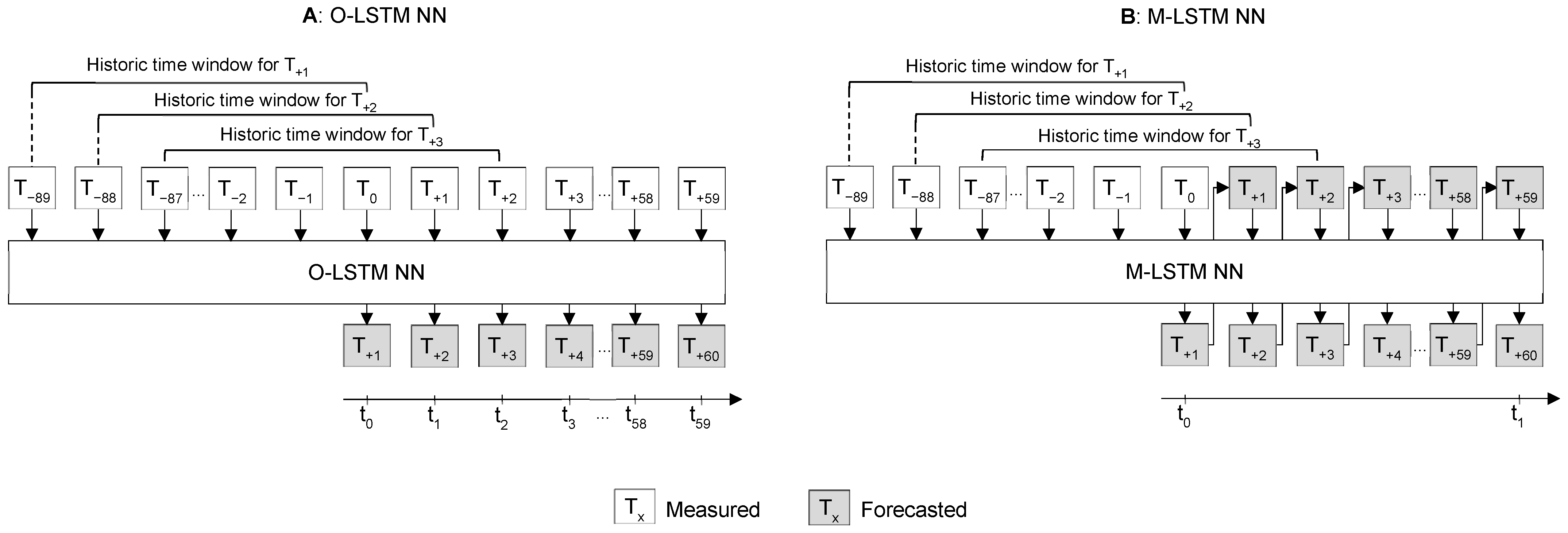
2.1. Machine Learning: LSTM Neural Networks for Intra-Hour Forecast

For intra-hour energy demand forecasting, two neural networks were investigated, aiming for monitoring the contracted grid capacity. In general, neural networks come in various types based on their intended applications. In the context of forecast modelling, Long Short-Term Memory Recurrent neural networks (LSTM-RNNs) prove particularly suitable in terms of short forecast horizons [22]. LSTMs, compared to standard RNNs, capture more extensive historical context (LSTMs < 1000 time steps vs. RNNs < 10). Memory blocks within hidden layers enable handling short- and long-term dependencies in time series data [22,23].

To establish mathematically describable relationships and define internal model parameters, the neural networks must undergo training. This process involves splitting data into training, validation, and test sets. While the proportions may vary, it is customary for training data to constitute approximately 75% to 80% of the dataset. In this study, we allocated 80% for training, 10% for validation data, and 10% for test data. Besides model parameters, so called hyperparameters, dictating the neural network’s structure (e.g., number of layers, nodes) and performance (e.g., learning rate), must be pre-defined before training [24]. In our work, we used the method GridSearch [25] for setting up the hyperparameters. Both neural networks, the O-LSTM NN and M-LSTM NN, consist of three layers, each employing up to 90 nodes. Implementation took place in Python using Keras, a high-level application programming interface (API) of the TensorFlow library. Besides optimizing the hyperparameters via GridSearch, the models are characterized by the following key parameters: a linear activation function, Mean Squared Error (MSE) for evaluating the loss function, and the ADAM optimizer.

The O-LSTM NN predicts the next value within the chosen time resolution (1 min) and thus serves a very short forecasting horizon (Figure 4A). Therefore, our model utilizes historical energy demand values within a defined time window (90 timesteps from the immediate past) as input to forecast the next value in the future (T₋₈₉ to T₀ for T₊₁). After the value for T₊₁ is measured in real-time, it is available for the forecast of the next time step. To forecast the future value for T₊₂, the time window of past values proceeds one step forward (T₋₈₈ to T₊₁). Therefore, the input side of the model contains only real measured values of the energy demand. In this manner, the forecast rolls along with the real time axis. To extend the forecast horizon, the M-LSTM NN comes into play. This starts like the O-LSTM NN but iterates, using the previous forecasted output as input for each subsequent step, enabling the forecast of multiple data points extending the forecasting horizon from 1 to 60 min in the investigated case (Figure 4B). It is important to note that as multi-step forecasts rely on previously predicted values, errors accumulate over time [26].

2.2. Statistic–Stochastic Model: SARIMA and Markov Chains for Day-Ahead Forecast

A hybrid model that combines statistical and stochastic methods has been developed for forecasting energy consumption, particularly for day-ahead electricity purchasing within a 36 h forecast horizon. This horizon aligns with the day-ahead market’s operational requirements, where knowledge of hourly resolved energy consumptions for the whole next day until 12 p.m. on the current day (market clearing) is crucial. The workflow for the statistic–stochastic model is illustrated in Figure 5.

Since the needed amount of electrical energy required for each heat depends heavily on the inserted scrap mass, it is necessary to forecast the future scrap masses for upcoming heats of the desired day-ahead time horizon. This is realized with a SARIMA model. A SARIMA model essentially combines an auto-regressive (AR) and a moving average (MA) approach. The AR component models observations based on historical behaviour, while the MA component constitutes a linear regression incorporating current time series values and historic process error values [27]. Initially rooted in economics, these approaches has gained extensive application in industrial and energy-related domains due to their versatility in modelling both deterministic and stochastic behaviours. For instance, SARIMA approaches were employed to forecast the heat demand in district heating systems [27], demand patterns in specific regions in Ghana [28], and short-term electrical loads in combination with Fast Fourier Transformation [29]. SARIMA models are characterized by seven main parameters: (p, d, q) (P, D, Q)_s. Here, p represents the order of auto-regression, d signifies the order of integration (or stationarity), and q denotes the moving average order. P, D, and Q refer to the same concepts as p, d, and q but are applied to the seasonal component of the time series. The seasonal period is denoted as s [30]. Parameters p and P are determined using the autocorrelation function (ACF), while q and Q are determined through the partial autocorrelation function (PACF). d and D are calculated using the Augmented Dickey–Fuller test. Parameter selection is highly contingent on the time series characteristics. In this specific case, the seasonality is set to 35, reflecting an average of 35 heats completed every 24 h across different days, indicating a certain degree of regularity. The parameters employed to predict scrap masses are (10, 0, 6) (3, 1, 4)₃₅.

In the next step, the needed energy amount is calculated through a linear regression relationship between scrap mass and energy consumption (Figure 6). After calculating the required overall energy consumption for future heats, the amount of energy is allocated across the heat’s operational phases based on historical data distributions (Table 1). The heat’s duration, along with its initiation and completion times, can be similarly derived from the predicted scrap mass.

Within the energy-relevant operating phases (three melting phases and fining), a Markov chain sequence in a 1 min resolution is generated using the previously calculated energy consumption and duration. The principle of generating Markov chains can be applied to model fluctuating energy consumers like EAFs. In the field of EAF steelmaking, Esfahani and Vahidi (2012) [31] utilized a Hidden Markov model to simulate the behaviour of the electric arc itself. Chen et al. (2003) [32] modelled the non-linear, highly time-varying load of an electric arc at least one step in advance using first- and second-order Markov-like models.

Processes involving time-resolved load profiles consist of a sequence of discrete states. In a sequence of observed states, there is a probability of transitioning from one state (i) to another (j) within one time step (n) (1). p_ij(n) represents this transition probability.

$$p_{ij}\left(n\right)=Prob\left\{X_{n+1}=j\right|X_n=i\},$$

(1)

To construct a Markov chain, these probabilities are organized in a matrix P. Each element of the matrix P(n) must satisfy two conditions: the probability of transitioning from one state to the next is less than 1, and the row-wise sum of all probabilities p_ij(n) equals 1 (Equations (2) and (3)).

$$0\le p_{ij}\left(n\right)\le 1,$$

(2)

$${\displaystyle {\sum }_{all j}}{p}_{ij}\left(n\right)=1,$$

(3)

Transition probabilities are cumulated using a specific equation to construct a Markov sequence. Starting with an initial state and a generated discrete random number z (0 ≤ z ≤ 1), the cumulated transition probability matrix determines the next state, which becomes the initial state for the next time step. A comprehensive explanation of Markov chains, including their construction and applications, can be found in the study by Stewart (2009) [33].

Before initializing the needed transition probability matrix, the data undergo preprocessing, including checks for heat completeness (presence of all six operational phases), correct operational phase order, and adequate heat length (between 30 and 60 min). Separate transition probability matrices are calculated for the three melting phases and the fining phase to account for their specific characteristics. Additionally, a search for the most common start values was performed for these phases to initialize the Markov sequences’ generation. This part of the model is also implemented in Python (PyCharm 2023.3.4), primarily utilising libraries such as NumPy, pandas, and statsmodels.

The Markov sequence for the whole heat is then segmented into the demand curves for electricity and natural gas in a last step. Since the natural gas demand shows a similar pattern across the heats, a third-order polynomial fit is employed to construct the natural gas demand curve. With a straightforward resampling algorithm, the demand curves can be aggregated into 1 h energy consumption values as a foundation for electricity procurement in the day-ahead market.

3. Results and Discussion

In this chapter, we present the results of the investigated forecast approaches and assess their accuracy and robustness using five different samples from the test dataset (Sample 1 to 5). Each forecast approach (O-LSTM NN, M-LSTM NN, and statistic–stochastic model) was applied to each of the five test samples. We employ the relative Root Mean Squared Error (rRMSE) and the Mean Average Percentage Error (MAPE) as error measures. By applying these error measures, we compare the known data with the generated forecasts in a quantitative manner. The RMSE captures the standard deviation of the residuals, while the rRMSE presents results in a percentage form and therefore enhances interpretability (Equation (4)). This measure considers the number of data points ($n$), the observed (real) values ($o_i$), the forecasted values ($f_i$), and the mean of the observed values ($\overline{o_i})$. The MAPE also expresses the forecast accuracy as a percentage (Equation (5)). These error measures are especially suitable for our study’s normalized data.

$$\mathrm{r}\mathrm{R}\mathrm{M}\mathrm{S}\mathrm{E}=\frac{\sqrt{\frac{1}{n}{\displaystyle {\sum }_{i=1}^n}(o_i-f_i)²}}{\overline{o_i}}·100\%,$$

(4)

$$\mathrm{M}\mathrm{A}\mathrm{P}\mathrm{E}=\frac{1}{n}{\displaystyle {\sum }_{i=1}^n}\frac{\left|o_i-f_i\right|}{o_i}·100\%,$$

(5)

The quantitative investigation focuses on two main aspects: the stability of the error measures over the forecast horizon and across the investigated samples. As the presented forecasting approaches aim at different objectives and markets, the target variables and considered periods for calculating the error measures differ (

Table 3. Target variable and time frame of error measures for investigated approaches.

Approach	Target Variable, Unit	Error Measure for …
O-LSTM NN	Energy Demand, MW	15 min
M-LSTM NN	Energy Demand, MW	15 min
Statistic–stochastic model
- SARIMA	Scrap mass, t	Hours (heats)
- Markov	Energy Consumption, MWh	One hour

). The rRMSE and MAPE are calculated for 15 min segments for the intra-hour approaches (O-LSTM NN and M-LSTM NN). We choose 15 min averages, since the pricing of the maximum contracted grid connection capacity for large industrial consumers is based on their maximum yearly 15 min average. Therefore, exceeding this average during production is linked to high additional costs. We evaluated the results based on the statistic–stochastic model (scrap masses as intermediate results and energy consumption) also with the rRMSE and MAPE but based on one-hour segments, since this is the usual unit to buy electricity on the spot market. Additionally, a monetary evaluation was conducted for the statistic–stochastic model in regard to two different methods of electricity procurement: standard load profile purchasing and forecast model purchasing.

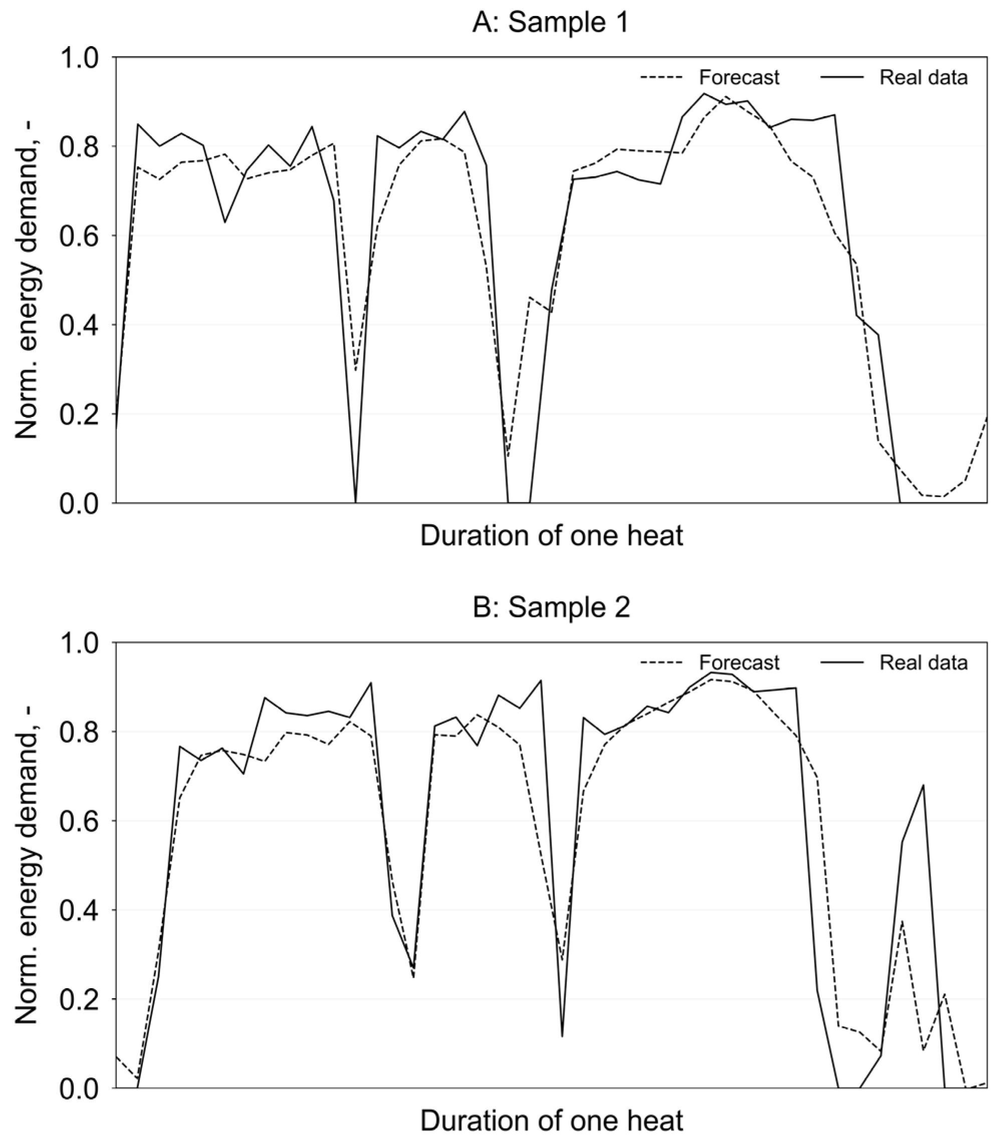
3.1. Intra-Hour Forecast

3.1.1. O-LSTM NN

For intra-hour forecasts, which serve as a guard for maximum contracted grid connection capacity, it is crucial to know the EAF’s energy demand in a temporally resolved manner to detect power peaks. The O-LSTM NN has a forecast horizon of one minute. Figure 7 shows the energy demand forecast for Sample 1 and 2 using the O-LSTM NN introduced in Section 3.1.1. Besides quantitative error measures, accurately representing the curve’s characteristics is important for the maximum guard function. Figure 7 demonstrates that the curve characteristic is appropriately modelled, distinguishing charging from melting phases and accurately depicting peaks during melting.

Looking at the rRMSE (

Table 4. O-LSTM NN: error measures in 15 min segments.

	rRMSE, %				MAPE, %
	0′–15′	15′–30′	30′–45′	45′–60′	0′–15′	15′–30′	30′–45′	45′–60′
Sample 1	3.71	1.02	3.42	11.97	11.75	0.95	2.94	7.66
Sample 2	1.30	8.44	6.16	41.43	1.64	7.55	5.40	41.59
Sample 3	7.97	0.73	6.50	-	5.87	0.60	15.90	-
Sample 4	10.00	14.83	2.05	2.76	7.33	14.36	2.09	17.71
Sample 5	30.38	16.29	0.17	3.22	25.06	25.13	0.18	2.55
Mean	10.67	8.26	3.66	11.88	10.33	9.72	5.30	17.38

), no significant pattern over the analysed five samples and the four considered time intervals is notable. In contrast, the MAPE increases in the last 15 min segment (45′–60′), with a mean of 17.38% across the samples. The other 15 min segments have mean MAPE values of 10.33% (0′–15′), 9.72% (15′–30′), and 5.30% (30′–45′). The higher error measures in the last segment are attributed to the fining phase at the end of a heat. During fining, the slag is formed, which primarily functions to remove unwanted components from the melt. The amount of unwanted components depends heavily on the quality of the inserted steel scrap and therefore varies widely for different heats. This results in a more error-prone forecast for this segment as information about the chemical composition of the scrap is not available. However, the fining phase shows considerably lower peak power compared to the melting phases. The maximum power demand of a heat will not be in this operational phase, which makes it not critical regarding the maximum contracted grid connection capacity. A comparison between the samples shows that the rRMSE ranges from 0.73% to 16.29% (with an outlier in Sample 2 (41.43%)) and that the MAPE ranges from 0.18% to 17.71%. There are no error measures for Sample 3 in the last 15 min segment, as the heat’s duration was less than 45 min. In summary, it can be stated that the O-LSTM NN approach works well for the considered samples.

3.1.2. M-LSTM NN

The results of the M-LSTM NN for Samples 3 and 4 are exemplarily shown in Figure 8. Notably, the charging phases between the melting phases are less accurately depicted compared to the O-LSTM NN. Furthermore, the forecasted curve appears much smoother than the real one.

Quantitative error measures (

Table 5. M-LSTM NN: error measures in 15 min segments.

	rRMSE, %				MAPE, %
	0′–15′	15′–30′	30′–45′	45′–60′	0′–15′	15′–30′	30′–45′	45′–60′
Sample 1	18.71	3.35	15.39	50.63	60.11	3.13	13.30	32.40
Sample 2	41.87	12.94	8.04	46.49	53.84	11.48	7.19	46.30
Sample 3	10.00	0.44	5.81	-	7.46	0.37	14.22	-
Sample 4	11.67	4.51	4.45	17.49	8.59	4.41	4.35	13.64
Sample 5	25.75	41.01	9.23	38.67	21.33	63.35	7.23	30.01
Mean	21.60	12.45	8.58	38.32	30.27	16.55	9.26	30.59

) reveal a pattern in the rRMSE results, where they are higher in the first and last segment (21.60% (0′–15′) and 38.32% (for 45′–60′)) and of a larger range from 0.44% to 50.63%. The MAPE also exhibits higher values in the first and last 15 min segments, with mean values over all samples of 30.27% and 30.59%. This suggests that the M-LSTM NN approach struggles to model the initiation and completion of a heat. The other 15 min segments have a mean MAPE of 16.55% (15′–30′) and 9.26% (30′–45′). Again, there are no error measures for Sample 3 in the last 15 min segment, as the heat’s duration was less than 45 min. Similar to the O-LSTM NN, the M-LSTM NN also faces challenges when representing the fining phase, primarily due to the same reasons mentioned in Section 3.1.1. Comparing samples, the average MAPE ranges from 9.26% to 30.59%, wider than that of the O-LSTM NN. Furthermore, the M-LSTM NN’s error measures are higher than those of the O-LSTM NN, indicating decreased forecast accuracy with an increasing forecast horizon length.

If a very brief time window (<1 min) suffices to react to a probable exceeding of the grid capacity, the O-LSTM NN approach prevails due to its higher accuracy over the M-LSTM NN. Should this action window be too short, the M-LSTM NN becomes the choice, as it is able to cover a longer future time horizon despite lower accuracy. It is essential to note that the M-LSTM NN approach can only work successfully when the forecast begins at the initiation of a heat. Starting calculations within a heat leads to unusable results because there is no possibility to give the model information about the actual EAF phase. Additionally, forecasting more than one heat into the future is problematic for this approach, as it cannot handle varying lengths of breaks between the heats. In contrast, the O-LSTM NN, while capable of displaying breaks between heats, is limited by a forecast horizon of just one time step, equivalent to one minute in this case.

3.2. Day-Ahead Forecast

To optimize electricity purchasing, we employed the combined statistic–stochastic model described in Section 2.2 for forecasting hourly energy consumption one day ahead. We evaluated the consumption forecast quantitatively with the introduced error measures and monetarily, considering two methods of electricity procurement: standard load profile purchasing and forecast model purchasing.

Table 6. SARIMA: error measures for forecasted scrap masses for different numbers of heats.

	rRMSE, %				MAPE, %
	10 Heats	20 Heats	30 Heats	60 Heats	10 Heats	20 Heats	30 Heats	60 Heats
	(App. 7 h)	(App. 14 h)	(App. 21 h)	(36(+) h)	(App. 7 h)	(App. 14 h)	(App. 21 h)	(36(+) h)
Sample 1	3.12	3.44	3.44	3.98	2.13	2.72	2.95	3.36
Sample 2	4.52	4.73	4.20	4.09	2.64	4.33	2.84	3.47
Sample 3	3.88	3.76	3.66	3.77	2.03	2.89	3.10	2.94
Sample 4	2.80	3.55	3.77	3.45	1.63	2.77	2.53	2.80
Sample 5	2.15	2.15	3.23	3.23	2.52	1.66	3.02	2.47
Mean	3.29	3.53	3.66	3.70	2.19	2.87	2.89	3.01

presents the results of the forecasted scrap masses, forming the foundation for the energy consumption forecast. To assess the approach’s robustness, we used the five same samples as discussed at the beginning of Section 3. Additionally, we explored different forecast horizons to evaluate the SARIMA approach’s suitability. On average, 52 heats span a 36 h period and, to ensure comprehensive coverage, extend a few hours beyond the intended time range (60 heats, 36(+)). This also mimics realistic procurement behaviour, allowing operational staff a window of time to make decisions before market clearing. Both rRMSE and MAPE exhibit a slightly increasing error pattern as the forecasted number of heats rises. With 10 (app. 7 h) heats, the mean rRMSE is 3.29%, while it increases to 3.70% with 60 heats (36(+) h). Similarly, the mean MAPE is 2.19% for 10 heats and 3.01% for 60 heats. These results suggest that forecast accuracy improves with a shorter horizon. Nonetheless, considering the desired application, the SARIMA approach with a 36(+) h forecasting horizon still provides satisfactory accuracy.

Table 7. Statistic–stochastic model: Error measures for forecasted energy consumption for different forecast horizons.

	rRMSE, %				MAPE, %
	10 Heats	20 Heats	30 Heats	60 Heats	10 Heats	20 Heats	30 Heats	60 Heats
	(App. 7 h)	(App. 14 h)	(App. 21 h)	(36(+) h)	(App. 7 h)	(App. 14 h)	(App. 21 h)	(36(+) h)
Sample 1	16.07	14.13	25.99	23.96	10.65	8.88	17.17	15.26
Sample 2	22.67	23.44	24.75	23.26	13.26	14.48	15.17	17.93
Sample 3	15.40	22.23	21.04	23.44	10.47	16.16	14.20	15.08
Sample 4	15.57	19.99	27.05	25.36	10.41	13.45	23.66	21.30
Sample 5	21.83	20.68	19.80	18.02	15.83	13.57	11.73	10.44
Mean	18.31	20.09	23.73	22.81	12.12	13.31	16.39	16.00

displays the error measures for the energy consumption forecast. As shown, the rRMSE (MAPE) increases with a longer forecast horizon, ranging from 18.31% (12.12%) to 22.81% (16.00%). This further confirms that forecasts become slightly less accurate as the forecast horizon extends. Observations reveal that there are larger discrepancies in the hourly forecasted energy consumption compared to the forecasted scrap masses. We attribute this to two main factors: Firstly, the correlation between scrap mass and energy consumption is not absolute. Secondly, the considerable volatility in scrap quality, particularly in its chemical composition, significantly influences the energy needed for scrap melting [7]. It is important to note that our investigations did not consider the chemical composition of used scrap due to the unavailability of the data.

In addition, a monetary evaluation was conducted to assess the model’s support for optimized energy procurement. Two scenarios were compared: electricity purchase based on the previous year’s load profile (standard load profile) and based on the results of the statistic–stochastic forecast model. Both scenarios involved buying electricity exclusively from the spot market, with any excess or shortfall traded on the energy balancing market. Electricity prices for the investigated period were obtained from the Austrian Power Grid AG, the Austrian electricity grid operator [34,35]. Figure 9 illustrates the comparison between the real data and standard load profile (A) and between the real data and forecast model results (B). Deviations are further detailed in

Table 8. Monetary evaluation for standard load profile and forecast model (positive (negative) values for MWh to be balanced describe excess (shortfall) energy and negative (positive) values for cost savings describe costs (profit)).

	Standard Load Profile		Forecast Model
	MWh to Be Balanced, %	Cost Savings, %	MWh to Be Balanced, %	Cost Savings, %
Sample 1	8.42	1.48	3.33	0.61
Sample 2	15.60	−3.39	1.23	−0.17
Sample 3	16.06	−3.82	−0.95	−0.66
Sample 4	14.20	−2.60	2.83	0.52
Sample 5	6.31	−0.47	−2.71	0.75
Mean	12.12	−1.76	2.21	0.21

. The results show that when electricity is procured based on the standard load profile, a substantial amount of energy must be balanced (12.12%, absolute mean across all samples, relative to the actual consumption). In contrast, utilising the forecast model for purchasing requires balancing only 2.21% of energy. Though the costs associated with balancing energy are subject to complex market conditions, it can be concluded that purchasing electricity using the forecast model can yield cost savings (0.21% mean per sample) compared to the procurement based on the standard load profile (−1.76% mean per sample, implying long-term costs for balancing energy on the energy balancing market). Furthermore, the approximately 2% difference in electricity costs between the two procurement scenarios amounts to hundreds of thousands of euros annually for an electric steel mill.

4. Conclusions

In energy consumption and demand forecasting, it is essential to recognize that no forecast is perfect. While traditional error measures offer a well-understood metric for assessing forecast accuracy, they may not fully capture the economic value of forecast errors. Evaluating energy forecasts accurately can be quite challenging, as they are utilized to influence or guide decision-making processes. The way forecasts are employed plays a significant role in evaluating forecast errors [10]. In this study, we addressed the research questions regarding energy consumption and demand forecasting for an EAF while pursuing two objectives: monitoring contracted grid connection capacity and optimising electricity purchasing for the day-ahead market. We demonstrated how to conduct a time series forecast of EAF energy usage, employing various methods for different forecast horizons. Furthermore, we presented the evaluation process to assess forecast quality in a qualitative, quantitative, and monetary manner.

For the intra-hour forecast, two approaches were considered: the O-LSTM NN and M-LSTM NN. The O-LSTM NN exhibited promising results in accurately modelling the energy demand curve, particularly distinguishing between charging and melting phases and capturing peak demand during melting phases. Quantitative analysis using error measures for 15 min segments showed good performance across the forecast horizon (mean rRMSE across all samples: 10.67% (0′–15′), 8.26% (15′–30′), 3.66% (30′–45′) and 11.88% (45′–60′)). However, the MAPE indicated a higher accuracy for the first three 15 min segments (10.33% (0′–15′), 9.72% (15′–30′), and 5.30% (30′–45′)) compared to the last segment (17.38% (45′–60′)), attributed to the challenges in predicting the fining phase accurately. Overall, the O-LSTM NN approach proved to be robust and effective across the investigated samples. The M-LSTM NN approach faced challenges in accurately representing the charging phases and exhibited a smoother forecasted curve compared to the actual data. Error measures for the M-LSTM NN were generally higher than those for the O-LSTM NN, indicating a decreased forecast accuracy with an increasing forecast horizon. The rRMSE results were as follows: 21.60% (0′–15′), 12.45% (15′–30′), 8.58% (30′–45′), and 38.32% (45′–60′). The MAPE showed a similar pattern with higher error measures in the first and last 15 min segment: 30.27% (0′–15′), 16.55% (15′–30′), 9.26% (30′–45′), and 30.59% (45′–60′). The M-LSTM NN approach required the forecast execution to start at the initiation of a heat and had limitations in handling breaks between heats, unlike the O-LSTM NN approach. Therefore, the results suggest that the M-LSTM NN approach may have limitations in its applicability and accuracy compared to the O-LSTM NN approach but offers the ability to forecast a wider time window into the future and supports processes where a longer time window is needed for decision making.

For the day-ahead forecast, we employed a combined statistic–stochastic model based on SARIMA and Markov chains to forecast hourly energy consumption. Evaluating the SARIMA part of the model for scrap mass forecasting revealed an increasing rRMSE (MAPE) as the forecast horizon grows, starting from 3.29% (2.19%) for app. 7 h (10 heats) to 3.70% (3.01%) for 36(+) h (60 heats). Nonetheless, even with a 36(+) h forecast horizon, SARIMA demonstrated satisfactory accuracy for our intended application. Predicting energy consumption based on the forecasted scrap masses showed increasing but still acceptable error measures with longer forecast horizons (8 to 36(+) h), also indicating reduced accuracy as the horizon extends. The rRMSE ranged from 18.31 % for 8 h to 22.81% for 36(+) h and the MAPE ranged from 12.12% for 8 h to 16.00% for 36(+) h.

In addition to the quantitative evaluation of the combined statistic–stochastic model, we conducted a monetary valuation to assess the practical impact of the forecast model on electricity procurement strategies. Comparing electricity purchases based on the standard load profile using the forecast model highlighted significant benefits in cost reduction (0.21% mean across all samples) and reducing energy balancing needs (2.21% of actual consumption for use of forecast model versus 12.12% for use of standard load profile).

Two main takeaways can be stated: As Makridakis et al. (2022) [11] noted, and as our study confirms, a longer forecast horizon tends to have a lower accuracy. Different forecasting methods exhibit varying rates of accuracy deterioration over extended horizons. Despite the challenges in accurately evaluating energy forecasts, our study contributes to understanding the performance of various methods in the specific context of EAF energy usage forecasting, considering grid capacity monitoring and optimized electricity purchasing objectives. The findings suggest that better-informed day-ahead scheduling for large (industrial) consumers could, besides offering a potential for cost savings, alleviate grid stress. This, in turn, might aid energy conservation by avoiding excess energy provision and, consequently, reduce CO₂ emissions through enhanced efficiency measures.

Moving forward, further investigations should be conducted with the models implemented at the industrial site. This requires ensuring a seamless data connection and developing an execution routine that integrates real-world trigger information. In the context of intra-day forecasting, accuracy is crucial, highlighting the necessity for a rolling horizon approach and the integration of feedback loops for real-time process monitoring and alignment with the forecasted information—a concept commonly known as digital twinning.

Since electric steel plants can differ greatly in terms of their production due to the steel qualities produced; these approaches must be tested with real production data from other electric steel plants in order to make a cross-industry statement.

To address forecasting challenges, potential improvements involve considering the chemical composition of the scrap. To facilitate this, it is recommended to enhance scrap sorting and scrap (quality) homogenisation processes. Furthermore, a higher degree of process automation could improve predictability in the EAF process. In conclusion, digitizing the EAF steelmaking process to enhance predictability and control offers opportunities for better integration of demand side management, improving energy efficiency and cost control.

References

1. Greening, L.A.; Boyd, G.; Roop, J.M. Modeling of industrial energy consumption: An introduction and context. Energy Econ. 2007, 29, 599–608. [Google Scholar] [CrossRef]
2. Paulus, M.; Borggrefe, F. The potential of demand-side management in energy-intensive industries for electricity markets in Germany. Appl. Energy 2011, 88, 432–441. [Google Scholar] [CrossRef]
3. International Energy Agency. Iron and Steel Technology Roadmap: Towards More Sustainable Steelmaking; International Energy Agency: Paris, France, 2021. [Google Scholar]
4. Fan, Z.; Friedmann, S.J. Low-carbon production of iron and steel: Technology options, economic assessment, and policy. Joule 2021, 5, 829–862. [Google Scholar] [CrossRef]
5. Marchiori, F.; Belloni, A.; Benini, M.; Cateni, S.; Colla, V.; Ebel, A.; Lupinelli, M.; Nastasi, G.; Neuer, M.; Pietrosanti, C.; et al. Integrated Dynamic Energy Management for Steel Production. Energy Procedia 2017, 105, 2772–2777. [Google Scholar] [CrossRef]
6. Chen, C.; Liu, Y.; Kumar, M.; Qin, J.; Ren, Y. Energy consumption modelling using deep learning embedded semi-supervised learning. Comput. Ind. Eng. 2019, 135, 757–765. [Google Scholar] [CrossRef]
7. Carlsson, L.S.; Samuelsson, P.B.; Jönsson, P.G. Modeling the Effect of Scrap on the Electrical Energy Consumption of an Electric Arc Furnace. Processes 2020, 8, 1044. [Google Scholar] [CrossRef]
8. European Ferrous Recovery and Recycling Federation. EU-27 Steel Scrap Specification; European Ferrous Recovery and Recycling Federation: Brussels, Belgium, 2007. [Google Scholar]
9. Carlsson, L.S.; Samuelsson, P.B.; Jönsson, P.G. Predicting the Electrical Energy Consumption of Electric Arc Furnaces Using Statistical Modeling. Metals 2019, 9, 959. [Google Scholar] [CrossRef]
10. Hong, T.; Pinson, P.; Wang, Y.; Weron, R.; Yang, D.; Zareipour, H. Energy Forecasting: A Review and Outlook. IEEE Open J. Power Energy 2020, 7, 376–388. [Google Scholar] [CrossRef]
11. Makridakis, S.; Spiliotis, E.; Assimakopoulos, V.; Semenoglou, A.-A.; Mulder, G.; Nikolopoulos, K. Statistical, machine learning and deep learning forecasting methods: Comparisons and ways forward. J. Oper. Res. Soc. 2022, 74, 840–859. [Google Scholar] [CrossRef]
12. Barker, J. Machine learning in M4: What makes a good unstructured model? Int. J. Forecast. 2020, 36, 150–155. [Google Scholar] [CrossRef]
13. Çamdalı, Ü.; Tunç, M. Modelling of electric energy consumption in the AC electric arc furnace. Int. J. Energy Res. 2002, 26, 935–947. [Google Scholar] [CrossRef]
14. Logar, V.; Dovžan, D.; Škrjanc, I. Mathematical Modeling and Experimental Validation of an Electric Arc Furnace. ISIJ Int. 2011, 51, 382–391. [Google Scholar] [CrossRef]
15. Zhou, D.; Gao, F.; Guan, X.; Chen, Z.; Li, S.; Lu, Q. Daily electricity consumption forecast for a steel corporation based on NNLS with feature selection. In Proceedings of the 2004 International Conference on Power System Technology, 2004. PowerCon 2004, Singapore, 21–24 November 2004; pp. 1292–1297. [Google Scholar] [CrossRef]
16. Andonovski, G.; Tomažič, S. Comparison of data-based models for prediction and optimization of energy consumption in electric arc furnace (EAF). IFAC-PapersOnLine 2022, 55, 373–378. [Google Scholar] [CrossRef]
17. Kovačič, M.; Stopar, K.; Vertnik, R.; Šarler, B. Comprehensive Electric Arc Furnace Electric Energy Consumption Modeling: A Pilot Study. Energies 2019, 12, 2142. [Google Scholar] [CrossRef]
18. Carlsson, L.; Samuelsson, P.; Jönsson, P. Using Interpretable Machine Learning to Predict the Electrical Energy Consumption of an Electric Arc Furnace. Stahl Eisen 2019, 139, 24–29. [Google Scholar]
19. Dock, J.; Janz, D.; Weiss, J.; Marschnig, A.; Kienberger, T. Time- and component-resolved energy system model of an electric steel mill. Clean. Eng. Technol. 2021, 4, 100223. [Google Scholar] [CrossRef]
20. Baumann, S.; Gnisia, M.; Feifel, P.; Klingauf, U. Identifikation und Behandlung von Ausreißern in Flugbetriebsdaten für Machine Learning Modelle. In Proceedings of the Deutscher Luft- und Raumfahrtkongress 2018, Friedrichshafen, Germany, 6 September 2018. [Google Scholar]
21. Visplore—Software for Visual Time Series Analysis, Visplore (v2023 a (1.5.2)); Visplore GmbH: Vienna, Austria, 2020.
22. Butt, F.M.; Hussain, L.; Mahmood, A.; Lone, K.J. Artificial Intelligence based accurately load forecasting system to forecast short and medium-term load demands. Math. Biosci. Eng. 2020, 18, 400–425. [Google Scholar] [CrossRef] [PubMed]
23. Staudemeyer, R.C.; Morris, E.R. Understanding LSTM—A Tutorial into Long Short-Term Memory Recurrent Neural Networks. arXiv 2019, arXiv:1909.09586v1. [Google Scholar]
24. Elgeldawi, E.; Sayed, A.; Galal, A.R.; Zaki, A.M. Hyperparameter Tuning for Machine Learning Algorithms Used for Arabic Sentiment Analysis. Informatics 2021, 8, 79. [Google Scholar] [CrossRef]
25. Carlsson, L.S.; Samuelsson, P.B.; Jönsson, P.G. Interpretable Machine Learning—Tools to Interpret the Predictions of a Machine Learning Model Predicting the Electrical Energy Consumption of an Electric Arc Furnace. Steel Res. Int. 2020, 91, 2000053. [Google Scholar] [CrossRef]
26. Taieb, S.B.; Sorjamaa, A.; Bontempi, G. Multiple-output modeling for multi-step-ahead time series forecasting. Neurocomputing 2010, 73, 1950–1957. [Google Scholar] [CrossRef]
27. Fang, T.; Lahdelma, R. Evaluation of a multiple linear regression model and SARIMA model in forecasting heat demand for district heating system. Appl. Energy 2016, 179, 544–552. [Google Scholar] [CrossRef]
28. Andoh, P.Y.; Sekyere, C.K.K.; Mensah, L.D.; Dzebre, D.E.K. Forecasting Electricity Demand in Ghana with the SARIMA Model. J. Appl. Eng. Technol. Sci. 2021, 3, 1–9. [Google Scholar] [CrossRef]
29. Musbah, H.; El-Hawary, M. SARIMA Model Forecasting of Short-Term Electrical Load Data Augmented by Fast Fourier Transform Seasonality Detection. In Proceedings of the 2019 IEEE Canadian Conference of Electrical and Computer Engineering (CCECE), Edmonton, AB, Canada, 5–8 May 2019. [Google Scholar]
30. Hu, W.; Tong, S.; Mengersen, K.; Connell, D. Weather variability and the incidence of cryptosporidiosis: Comparison of time series poisson regression and SARIMA models. Ann. Epidemiol. 2007, 17, 679–688. [Google Scholar] [CrossRef] [PubMed]
31. Esfahani, M.T.; Vahidi, B. A New Stochastic Model of Electric Arc Furnace Based on Hidden Markov Model: A Study of Its Effects on the Power System. IEEE Trans. Power Deliv. 2012, 27, 1893–1901. [Google Scholar] [CrossRef]
32. Chen, F.; Sastry, V.V.; Venkata, S.S.; Athreya, K.B. A Robust Markov-Like Mode for Three Phase Arc Furnaces. Caribb. Colloq. Power Qual. 2003, 2003, 1–6. [Google Scholar]
33. Stewart, W. Probability, Markov Chains, Queues, and Simulation: The Mathematical Basis of Performance Modeling; Princeton University Press: Princeton, NJ, USA, 2009. [Google Scholar]
34. Austrian Power Grid AG. Ausgleichsenergiepreise. Available online: https://markttransparenz.apg.at/markt/Markttransparenz/Netzregelung/Ausgleichsenergiepreise (accessed on 4 November 2023).
35. Austrian Power Grid AG. Day-Ahead Preise. Available online: https://markttransparenz.apg.at/markt/Markttransparenz/Uebertragung/EXAA-Spotmarkt (accessed on 4 November 2023).
Figure 1. Representative energy demand for two heats of the investigated EAF.
Energies 17 01326 g001
Figure 2. Forecast model classification scheme.
Energies 17 01326 g002
Figure 3. Impact area of different forecast horizons.
Energies 17 01326 g003
Figure 4. Model execution flow of O-LSTM NN (A) and M-LSTM NN (B).
Energies 17 01326 g004
Figure 5. Workflow of statistic–stochastic model.
Energies 17 01326 g005
Figure 6. Heat-wise EAF energy consumption based on inserted scrap mass using linear regression (regression line: grey line; whole dataset: transparent data points; representative sample of one week: solid data points).
Energies 17 01326 g006
Figure 7. Energy demand forecast of Sample 1 (A) and 2 (B) with O-LSTM NN.
Energies 17 01326 g007
Figure 8. Energy demand forecast of Sample 3 (A) and 4 (B) with M-LSTM NN.
Energies 17 01326 g008
Figure 9. Comparison of real data with the forecast (A) and the standard load profile (B) of the day-ahead electricity consumption for Sample 1.
Energies 17 01326 g009