
Predictive Energy Management of a Building-Integrated Microgrid: A Case Study


Processes, Materials and Solar Energy (PROMES-CNRS) Laboratory, University Perpignan Via Domitia, Rambla de la Thermodynamique, Tecnosud, 66100 Perpignan, France
*
Author to whom correspondence should be addressed.
Energies 2024, 17(6), 1355; https://doi.org/10.3390/en17061355
Submission received: 5 February 2024
/
Revised: 5 March 2024
/
Accepted: 9 March 2024
/
Published: 12 March 2024
(This article belongs to the Special Issue Advanced Control, Operation and Energy Management of Distribution Networks and Smart Grids)
Abstract
:The efficient integration of distributed energy resources (DERs) in buildings is a challenge that can be addressed through the deployment of multienergy microgrids (MGs). In this context, the Interreg SUDOE project IMPROVEMENT was launched at the end of the year 2019 with the aim of developing efficient solutions allowing public buildings with critical loads to be turned into net-zero-energy buildings (nZEBs). The work presented in this paper deals with the development of a predictive energy management system (PEMS) for the management of thermal resources and users’ thermal comfort in public buildings. Optimization-based/optimization-free model predictive control (MPC) algorithms are presented and validated in simulations using data collected in a public building equipped with a multienergy MG. Models of the thermal MG components were developed. The strategy currently used in the building relies on proportional–integral–derivative (PID) and rule-based (RB) controllers. The interconnection between the thermal part and the electrical part of the building-integrated MG is managed by taking advantage of the solar photovoltaic (PV) power generation surplus. The optimization-based MPC EMS has the best performance but is rather computationally expensive. The optimization-free MPC EMS is slightly less efficient but has a significantly reduced computational cost, making it the best solution for in situ implementation.
1. Introduction
The main grid is undergoing a gradual shift from a centralized to a decentralized structure. This is mainly due to the large-scale deployment of renewables, whose successful integration into the grid can be achieved through electrical/thermal/multienergy microgrids (MGs), including building-integrated microgrids (BIMGs), sometimes called nanogrids [1]. Electrical MGs can be defined as multiple parallel-connected distributed generators with coordinated control strategies that are able to operate either in grid-connected or islanded mode. Greater flexibility is crucial for grid-connected MGs as it allows local management of renewable energy sources and makes buildings more energy-efficient and sustainable. The U.S. Department of Energy defines an electrical MGs as “a group of interconnected loads and distributed energy resources within clearly defined electrical boundaries that acts as a single controllable entity with respect to the main grid”. For its part, the French Energy Regulation Commission (CRE) defines electrical MGs as “small-scale power grids designed to provide a reliable power supply to a small number of consumers”. Because renewable energy sources, like solar and wind, are diffuse and intermittent, storage systems are needed. Energy storage makes it possible to compensate for the intermittent nature of these renewable energy sources and increases their penetration into the grid. However, the most commonly used storage systems—electrochemical batteries—are still expensive [2]. According to the EDF (Electricité de France) [3], “thermal microgrids are buildings, clusters of buildings or district energy systems that combine heat recovery and storage, renewable energy sources, and power management through smart and distributed communications and control techniques”. According to the French Energy Regulation Commission [4,5,6], “the microgrid concept, likely to concern different system scales (i.e., a building, a district, an industrial or a craft zone, a village, etc.), is being extended to heat and natural gas networks, and can thus be thought out in a multifaceted manner”. The building sector accounts for around 30% of the world’s energy consumption [7]; thermal energy is responsible for more than 75% of this consumption [7]. According to the U.S. Department of Energy [8], heating, ventilation, and air-conditioning (HVAC) is about one-third of a building’s energy consumption in the United States of America. As an interesting solution to reduce the use of fossil fuels, solar hot water systems for space heating are booming [7]. As a result, the development of tools for improved HVAC design and operation has become a popular topic among researchers these past few years. On a wider scale, research activities dealing with the (smart) management of thermal resources and users’ thermal comfort in buildings are numerous. Regardless of the MG type and size, efficient strategies for energy resource management are needed. These strategies can be implemented through energy management systems (EMSs), i.e., automation systems designed to achieve energy efficiency through process optimization, taking advantage of energy measurements from the field. According to the International Electrotechnical Commission (IEC), an EMS is “a computer system comprising a software platform providing basic support services and a set of applications providing the functionality needed for the effective operation of electrical generation and transmission facilities so as to assure adequate security of energy supply at minimum cost” [9]. According to the International Organization for Standardization (ISO), “an energy management system involves developing and implementing an energy policy, setting achievable targets for energy use, and designing action plans to reach them and measure progress. This might include implementing new energy-efficient technologies, reducing energy waste or improving current processes to cut energy costs” [10]. In electrical/thermal/multienergy MGs, EMSs play a key role in the efficient management of distributed generators and energy storage systems in both grid-connected and islanded operation modes [11,12,13,14].
In [15], Chen et al. propose an MPC strategy for the management of a multisource MGs that combines electrical, thermal, and gas systems. Economic dispatch, which is a mechanism for determining the best cost-effective point of operation for all controllable devices, is performed. The proposed MPC strategy provides better results in simulation than conventional methods. In [16,17], a fuzzy energy management strategy is developed for enhancing the energy self-consumption of a residential multienergy (thermal/electrical) MG, taking advantage of a possible power generation surplus through heat storage. In [3], an MPC controller is developed for the management of the multienergy MG the Standford facilities are equipped with. The authors aim to reduce the economic cost of energy consumption, the environmental impact of the facilities, water usage, and the reliance on fossil fuels. In [18], both the steady-state model and the optimization scheduling formulation allowing the integrated operating cost of a multienergy MG to be minimized are presented. In [19], a demand-side management (DSM)-based energy management strategy is proposed by Pascual et al. in the context of a residential MG equipped with photovoltaic solar panels, a small wind turbine, and solar thermal collectors. The power exchanged with the main grid is managed using batteries and a controllable electric water heater. An improved grid power profile is achieved while reducing the overall cost of the system (mainly thanks to a smaller battery) by using forecasts and controlling the electric water heater. In [20], Tang et al. present a model predictive control approach aiming at reducing the power bought from the main grid but also satisfying thermal comfort constraints in a multienergy building-integrated MG. Thanks to the proposed approach, the power consumption is controlled and the thermal comfort temperature is satisfied. A simplified model is used, with no significant impact on the results. In [21], Kia et al. propose an optimal scheduling approach for thermal and electrical power generations in a multienergy MG. A gap decision theory method is employed to handle uncertainties. The strategy is able to operate the system in a robust/opportunistic way. As a result, either robustness is improved or the economic cost is reduced. In [22], Chen et al. propose a novel cumulative relative regret decision-making strategy for the robust optimization of a multienergy MG. The proposed approach is compared with a standard robust optimization approach, stochastic programming, and a minimum worst-scenario regret (MWR) strategy. Thanks to such an approach, robustness is ensured and the economic cost is reduced. Even if networked multienergy MGs are quite uncommon systems, Zhong et al. [23] have developed a day-ahead scheduling strategy with the aim of reducing both the economic cost and the emissions in a simulation. In [24], Hirao et al. propose an MPC strategy to manage a ground-source heat pump used to heat different buildings. The proposed approach is optimization-free. Once production and consumption forecasts are provided to the MPC controller, it selects among the different heating modes the one to be used. According to the authors, the proposed approach can be implemented in a real urban environment. In [25], Garnier et al. present an MPC strategy with low computational cost to manage thermal comfort in a nonresidential building. The idea behind the strategy is to identify the right instant to turn on/off the HVAC system in order to satisfy thermal comfort constraints during occupancy periods. The EnergyPlus software (version 8.1.0) was used to model the system. Thanks to the proposed approach, energy consumption is reduced, while the users’ thermal comfort is satisfied. In [26], Violante et al. present an MPC-based EMS dedicated to the management of isolated multienergy MG. The aim is to minimize the cost related to the use of fossil fuels and satisfy thermal comfort constraints. A real testbed was used to validate the EMS, allowing energy consumption to be reduced while preserving thermal comfort. In this work, nonuniform time intervals are used to reduce computation time. Finally, review papers on heat pump control strategies are proposed by Pean et al. [27] and Fischer et al. [28]. Rule-based strategies, which are easy to implement, and predictive strategies, which offer improved performance but can be computationally expensive, are reviewed, among other strategies for heat pump control.
The Interreg SUDOE project IMPROVEMENT (Integration of Combined Cooling, Heating and Power Microgrids in Zero Energy Public Buildings with High Power Quality and Continuity Requirements) was launched at the end of the year 2019 (www.improvement-sudoe.es) with the aim of turning public buildings with critical loads (i.e., hospitals, research centers, military facilities, etc.) into net-zero-energy buildings (nZEBs) by integrating multienergy MGs. The project is supported by the European Regional Development Fund (ERDF) and takes advantage of real case studies. The ERDF operates as part of the European Union’s economic, social, and territorial cohesion policy. It aims to strengthen economic and social cohesion in the European Union by correcting imbalances between regions. IMPROVEMENT is briefly presented in the following section. An overview of the work presented in this paper—this work deals with the development of a predictive EMS for the management of thermal resources and users’ thermal comfort in a public building equipped with a multienergy MG—is given as well [29]. This paper is organized as follows: Section 2 deals with the Interreg SUDOE project IMPROVEMENT. The case study is described in Section 3. The models of the thermal MG components are presented in Section 4. Section 5 depicts the energy management strategies and the control results. The paper ends with a conclusion and an outlook on future work (Section 6).
2. Interreg SUDOE Project IMPROVEMENT
2.1. Specific Objectives of the Project
As mentioned previously (see Section 1), the main objective of the Interreg SUDOE project IMPROVEMENT was to turn public buildings with critical loads into nZEBs by integrating multienergy MGs with combined heat, cooling, and power generation and storage systems. The project has three specific objectives, defined as follows [30]: (1) improve energy efficiency in public buildings through the development of a solar heating and cooling generation system and the incorporation of active and passive techniques; (2) develop a fault-resilient power management system for multienergy MGs under criteria of high-quality supply design; and (3) develop an EMS for renewable generation MGs equipped with hybrid energy storage under criteria of minimum degradation, maximum efficiency, and prioritization in the use of renewable energy.
Two pilot buildings were under investigation in the project. The first one is located in Lisbon, Portugal, and the second one is located in Puertollano, Spain. Only the Lisbon pilot building, which houses the National Energy and Geology Laboratory (LNEG), is considered in this work. This building-integrated MG is multienergy (see Section 3).
2.2. Contribution to the Project
The main contribution to the project is an advanced EMS based on model predictive control (MPC), developed using data collected in situ. The aim behind the IMPROVEMENT EMS is to manage the building’s thermal resources and users’ thermal comfort in a predictive way. To this end, optimization-free/based MPC controllers were developed and evaluated in simulation. The management of thermal resources relies on controlling both an air-to-water heat pump and a thermal energy storage while the management of users’ thermal comfort relies on controlling fan coil units. Optimization-free MPC controllers are paramount in controlling the computational cost associated with managing the building energy resources. In addition, it is worth mentioning the following aspects.
- The way the interconnection between the thermal part and the electrical part of the building-integrated MG can be managed is discussed. An interesting option, which is considered in this work, is to take advantage of a possible PV power generation surplus, which can be stored in a thermal energy storage system [2,31].
- The IMPROVEMENT EMS has to be ready for in situ implementation. To this end, the EMS takes advantage of existing controllers. The core idea behind its development is to supervise PID and RB controllers with MPC controllers in order to achieve optimal energy efficiency in public buildings equipped with multienergy MGs.
3. Case Study
3.1. Description of the LNEG Building-Integrated MG
The case study is the LNEG building-integrated MG located in Lisbon, Portugal [30]. The MG components are shown in Figure 1. Regarding the electrical MG, PV solar panels provide electricity to feed the loads or to charge a bank of batteries. The energy stored in the batteries can be discharged to meet the loads. However, if the electrical resources are not sufficient, the main grid can supply electricity to the electrical MG, which is connected to the thermal MG via an air-to-water heat pump (HP). The HP is powered by the main grid or using the PV power generation surplus coming from the electrical MG. In the thermal MG, solar collectors (SCs) supply heat to a hot water tank (HWT), which in turn supplies heat to a thermal energy storage (TES). The HP can also supply heat to the thermal energy storage. Finally, fan coil units (FCUs) use the heat coming from the TES to heat the different rooms in the building (Figure 2). The facility has two individual offices, R1 and R2 (11 each), a meeting room R3 (22 ), and a multipurpose room, R4 (83 ), for a total surface area of 170 . R1, R2, and R3 have standard single-glazed windows. R4 has two wide single-glazed windows and is often used for technical sessions and scientific presentations. Phase change materials are used to regulate the thermal inertia of the glazed areas (for both the southwest and northeast walls of R4), and highly efficient thermal and acoustic insulation panels are installed in the false ceiling. R1 is considered in this work, even if the room is not equipped with an air temperature sensor. In addition, R1 and R2 are very similar, which is why the results obtained for R2 are replicated to R1. The electrical MG is composed of 4 kWp solar photovoltaic panels and a 30 kWh bank of batteries. In the thermal MG, there are two hot water tanks: the first one (the HWT) is heated by the SCs and supplies heat to the second one (the TES). The TES is heated by the HP as well. The characteristics of the thermal MG components are as follows:
- The total surface of the evacuated tube SCs is 4 ;
- The HWT—a BAXI (Lisbon, Portugal) FST 300 accumulator—has a capacity of 300 L;
- The TES—a Lapesa (Lisbon, Portugal) G1000IS accumulator—has a capacity of 1000 L;
- The air-to-water HP—a Daitsu (São João da Talha, Portugal) CRAD 2 UiAWP 60 T—has a power of 16 ;
- The fan coil units are the Daitsu FDLA AC TS 3IFD2007 (×2), the Daitsu FMCD EC TOTAL 3IFD2010, and the Daitsu FDLA AC TS 3IFD5037.
3.2. Operation of the LNEG Pilot Building
In the LNEG pilot building, the bank of batteries does not have a high power of charge, and power consumption is very low, resulting in a high PV power generation surplus compared with the overall production. That is why the idea of using this surplus to supply the HP is interesting in this case study. However, if there is no PV power generation surplus, the main grid supplies electricity to the HP. If the PV panels and the bank of batteries do not supply enough electricity to meet the needs of the building, electricity is bought from the main grid. The FCUs are used to heat rooms R1, R2, R3, and R4, according to the following three operation modes:
- 1.
- The economic mode: Heat can be accumulated in the TES using two sources, the SCs and the HWT or the HP. The heat stored in the TES is then transferred to the rooms.
- 2.
- The economic mode with disconnected SCs: Heat can be accumulated in the TES only using the HP. The heat stored in the TES is then transferred to the rooms.
- 3.
- The direct mode: No heat is stored in the TES, only the HP supplies heat to the rooms through the FCUs. Only this mode is considered in this work in order to take advantage of the SCs the building is equipped with.
3.3. Operation Data
Operation and meteorological data are collected in situ thanks to the measuring devices the pilot building is equipped with. The sampling time is 10 min. Using data from the year 2022, the models were developed and simulations were performed. The data are consistent. There are only a few issues in the database: the missing data represent less than 0.3%, which is not a problem as the amount of data is large, with the exception of some weather quantities (global irradiance, outdoor temperature, and air humidity, to name a few), and outliers are almost not present. The following quantities are measured in situ:
- Power consumption ();
- PV power generation ();
- Outdoor temperature ();
- The air temperature in the rooms of the building ();
- The temperature of the water in the 4th layer of the HWT ();
- The temperature of the water in the 1st layer of the TES ();
- The temperature of the water in the 4th layer of the TES ();
- The temperature of the water circulating between the HWT and the TES () and the temperature of the water circulating between the TES and the FCUs ();
- The flow rate of the water circulating between the HWT and the TES (), the flow rate of the water circulating between the TES and the FCUs (), and the flow rate of the water circulating between the HP and the TES ().
4. Thermal MG Modeling
4.1. Literature Review on Thermal MG Modeling
Efficient controllers are needed to improve the energy efficiency of thermal MGs. In this context, computationally tractable functional models of the systems the MG is equipped with are essential to the controllers’ design and evaluation. Numerous efforts are being made to develop control-oriented models [32,33]. Data-based modeling and first-principle-based modeling are the two main modeling categories in this field. Data-based models do not require detailed knowledge about the underlying process but correlations are only valid within the range of the dataset used. In contrast, first-principle-based models reflect physical laws. Such models are difficult to build but have superior generalization capability. The modeling of solar-energy-based systems for space heating is addressed in the literature, but to the best of the authors’ knowledge, there are very few papers describing the full stack of components as an integrated model that can be used to develop and validate advanced energy management strategies. In [32], Pasamontes et al. have decided for hybrid modeling to describe the behavior of a solar thermal energy system composed of several subsystems. The thermal flat solar collector field, the hot water accumulation system, and the gas heater are modeled using first-principle-based equations. The discrete dynamics are also included in the model of the whole system. More recently, Gerard et al. [33] realized a study dealing with thermal comfort in a building equipped with a solar water heater consisting of thermal collectors, a water storage tank, a boiler, and a low-temperature radiator. The Bond Graph formalism—a graphical representation of first-principle equations allowing the development of state-space representations of physical systems—has been used to model the solar water heater. A few years ago, solar combined heat and power systems were reviewed by Kasaeian et al. [34], with a focus put on combined solar–heat pump systems for space heating. This work suggests that integrated modeling needs to be improved for better economic and environmental assessment.
4.2. Thermal MG Components Modeling
Data were collected at the LNEG pilot building and used to develop and validate simulation models of the solar hot water system components. The layout of the LNEG pilot building is shown in Figure 1. The thermal MG is shown in Figure 2. Mass and energy balance equations [35,36] are used to explain the units’ thermal behavior.
4.2.1. Evacuated Tube Solar Collectors
The pilot building is equipped with evacuated tube SCs. This kind of system is well suited to hot water heating applications. The SCs capture the radiant solar energy and convert it into thermal energy. This energy is transferred through a fluid. The precise modeling of the evacuated tube SCs [37] can result in a high computational cost when used along optimization-based strategies. Even if simplified models exist [38,39], the model proposed by Buzas et al. [35] is used, as the main interest of this model is to provide the temperature of the heat transfer fluid. As there is no accumulation of mass in the SCs, only the energy balance equation is considered. is the energy absorbed by the SCs, is the energy carried by the heat transfer fluid, and is the energy loss to the atmosphere by the SCs. The energy balance of the SCs is defined in the following way (1):
The energy absorbed by the SCs is as follows (2):
where is the SCs surface area (), is the optical efficiency (dimensionless), and I is the global tilted irradiance (GTI), measured with an angle of 45° () [35].
The energy carried by the heat transfer fluid () is as follows (3):
where is the mass flow rate of the heat transfer fluid (), is the specific heat capacity of the heat transfer fluid (), and and are the inlet and outlet temperatures, respectively.
Finally, the heat loss in the SCs is given by the following Equation (4):
where is the heat loss coefficient (), is the SCs surface area (), and is the absolute temperature of the SCs surface.
Since it is quite challenging to measure the surface temperature, for simplicity, the absolute temperature is approximated in Equation (5), with the outdoor temperature:
The mass flow rate is expressed in terms of volumetric flow rate (), as , with the heat transfer fluid density. Hence, after further rearranging of Equation (6), the final formulation is as follows (7):
From an automatic control perspective, the GTI (measured with an angle of 45°) I and the outdoor temperature are disturbances, while the heat transfer fluid inlet and outlet temperatures ( and ) are controlled variables, and the heat transfer fluid flow rate is a manipulated variable.
4.2.2. Hot Water Tank and Thermal Energy Storage Tank
The LNEG pilot building has a hot water tank (HWT) and a thermal energy storage (TES), equipped with heat exchangers. Heat storage relies on a stratification process, where hot water sits on cold water, as depicted in Figure 3 (HWT) and Figure 4 (TES). The SCs heat the water in the HWT directly. Then, the HWT provides heat to the FCUs, which are supplying heat to the rooms, via the TES. During the night or in case of cloudy conditions, continuous space heating is ensured thanks to the TES. The TES allows shifting energy consumption from on-peak to off-peak hours as well, significantly improving system performance and reducing the economic cost. A similar modeling approach, which is based on the energy balance equations, is considered for both the HWT and the TES. In this work, the node-based energy balance method is used, i.e., the energy balance equation for each node (12 in this case) is evaluated in [40,41]. The terms “node” and “layer” are interchangeably used in the literature, and the term “layer” is chosen for convenience here.
The following assumptions are made for model simplification [42]:
- The fluid used in the tanks is incompressible;
- The pressure in the tanks is assumed to be appropriate to avoid fluid phase changes;
- The mixing of layers due to buoyancy force is considered as negligible;
- There is no mass flowing in or out of the systems; hence, the mass balance equation is not considered.
As can be observed in Figure 3 (HWT), the fluid coming from the SCs circulates in the HWT heat exchanger, from layer 1 to layer 12. As can be observed in Figure 4 (TES), the water coming from the HWT (layer 1) circulates in the TES heat exchanger, from layer 6 to layer 10. Then, this water is back to the HWT (layer 12). The water circulating in the HP enters the top of the TES (layer 1) and leaves it at the bottom (layer 12), without circulating in a heat exchanger. The stored water leaves the TES from the top (layer 1), circulates through the FCUs, and then comes back to the bottom of the TES (layer 12). The temperature of the water in layer j is calculated from the respective temperatures of the water in layers and , as well as the temperature of the fluid circulating in the heat exchanger (layer j).
The energy balance for layer j is given by Equation (8), where , , and are the temperatures of the water in layers , j, and of the HWT (), respectively; is the flow rate of the water circulating between the HWT and the TES (); is the volume of the HWT (); is the density of water (); is the specific heat capacity of water (); is the HWT overall heat loss coefficient (); is the overall heat transfer coefficient of the HWT heat exchanger (); is the HWT cross-sectional surface of a layer (); is the air temperature in the thermal storage room of the LNEG pilot building in Lisbon, Portugal; and is the height of a layer in the HWT ():
In [41], Nash et al. introduce , (i.e., the internal heat transfer coefficients between layers), and (i.e., the internal heat transfer scaling parameter) in order to force the heat to be transferred downward or upward. These coefficients are calculated as follows using Equations (9) and (10):
The layers in contact with the water coming from the SCs (layer 1) or the TES (layer 12) (i.e., boundary layers of water in the tank) have specific equations. As hot water comes from the SCs, with being the temperature of the water leaving the collectors (this water is considered as layer 0 in the developed model), layer 1 has the following Equation (11):
As the cold fluid comes from the TES, with being the temperature of the water entering the HWT (this water is considered as layer 13 in the developed model), layer 12 has the following Equation (12):
Equations (8), (11), and (12) describe the dynamic behavior of the stratified HWT. It is worth mentioning that all the model parameters are derived from the available data (collected in the LNEG pilot building). To describe the dynamic behavior of the hot fluid circulating in the heat exchanger, Equations (13) and (14) are used for layer 1 and layer j, respectively:
where is the flow rate of the hot fluid circulating in the HWT heat exchanger (), is the density of the fluid (), is the specific heat capacity of the fluid (), is the volume of the HWT heat exchanger (), and is the overall heat transfer coefficient of the HWT heat exchanger ().
Regarding the TES, which has the same equations as the HWT, the influence of the HP has to be taken into consideration. As a consequence, a change is made to the model as the water circulating in the HP enters the first layer of the TES (15) and is mixed with the water already in the tank, and is added. The water coming from the HWT enters the TES at layer 6, through the heat exchanger, and leaves it at layer 10:
where is the flow rate of the water circulating between the FCUs and the TES (), is the flow rate of the water circulating between the HP and the TES (), is the volume of the TES (), is the TES overall heat loss coefficient (), and is the TES cross-sectional surface of a layer ().
4.2.3. Fan Coil Units
Fan coil units (FCUs) are HVAC systems widely used in buildings because they are easy to install, provide mounting versatility, and have low noise levels. A typical FCU is composed of a supply fan, a heat exchanger coil, filters, and noise alternators. In the heating coil, the supply air temperature is increased to the predefined temperature. This conditioned air is then used to heat the building’s thermal zones during occupancy periods. Note that the air filters do not directly affect the air temperature in a thermal zone; hence, the filters’ dynamics are neglected. The heat exchanger is a high-efficiency shell-and-tube-type heating coil. The mathematical model of this air-to-water heating coil—the energy balance equation is applied to both the shell- and tube-side fluid flow rates—is given by Equations (16) and (17). The hot water in the shell coming from the tanks heats the supply air in the tube side to the required temperature. In [43,44], the authors present a heat exchanger model that has been adapted to the system the LNEG pilot building is equipped with. A more detailed model has been developed by Bastida et al. [45], but such a complex model is not necessary in this work and would result in a higher computational cost. The required flow rate of the supply air entering the thermal zones is manipulated through the thermal zone controller. Note that the heat loss to the outside environment is considered negligible. Equations (16) and (17) deal with the dynamic behavior of the heat exchanged between the shell- and tube-side fluids for the cocurrent flow [43]:
where and are the inlet and outlet water temperatures of the stratified TES (), respectively, and are the inlet and outlet air temperatures of the heating coil (), respectively, and are the water and supply airflow rates (), respectively, is the volume of the heating coil (), is the volume of room z (), and are the tube/air-side and shell/water-side areas (), respectively, is the FCU conductive heat transfer coefficient (), is the length of the tube (), is the density of water (), is the specific heat capacity of water (), is the density of air (), and is the specific heat capacity of air ().
4.3. Thermal Zones Modeling
In this work, focus is put on the air temperature in the rooms as a thermal comfort indicator. There are four rooms of interest in the building, defining four thermal zones. The RC model (18), which is based on the first law of thermodynamics, is used for modeling these thermal zones [44,46]:
where is the air temperature in the room z () (in this study, is considered to be equal to ), is the flow rate of the supply air entering room z (), is the volume of room z (), is the supply air temperature (), is the outdoor temperature (), is the absolute thermal resistance of the walls of room z (), is the space occupied by a person in room z (), is the solar aperture of room z (), I is the solar irradiance (), is the solar transmittance of the window in room z (-) [47,48], and .
In addition, an internal heat gain q of 70 is considered for each person—a person with an office activity has a metabolic activity equivalent to 1 [25]—in the building. The same metabolic activity is considered in each room as activities are all the same. Simulations are performed by considering one person in room R1, one person in room R2, four (or more) persons in room R3, and sixteen (or more) persons in room R4. Let us note that thermal modeling could be improved by taking into consideration quantities like the walls’ temperature, the air temperature in adjacent rooms, the temperature of the ceiling surface, or the ground temperature. Due to limitations in the instrumentation of the building, it was not possible to carry this out at all.
4.4. Model Validation
4.4.1. Criteria
The derived mathematical models were simulated using numerical data from the LNEG pilot building. Model validation (see Table 1) was performed with site data and evaluated using the root-mean-square error (RMSE). The RMSE is defined as the square root of the average of squared errors and is given in Equation (19):
where n is the number of data points, is the measured data , and is its corresponding estimation. For more information on the RMSE, the interested reader is referred to [49].
The normalized root-mean-square error (nRMSE) formulation is given in Equation (20):
where and are the maximum and minimum values of the measured data, respectively.
4.4.2. Thermal Zone Modeling: Results
The validation of the thermal zones model was conducted without turning on the FCUs. The FCUs are not used on weekends, so, in order to validate the model, these periods are considered. Validation with the FCUs turned on is not possible, as the flow rate of the water circulating in the FCUs and the FCU supply air flow rate are not measured. The GTI (measured with an angle of 45°) and outdoor air temperature have been used as model inputs. In addition, the solar aperture is modified in order to correct the irradiance entering the rooms. Because global irradiance is measured on the roof of a building that is not the LNEG pilot building, some empirical adjustments have been made to obtain appreciable results regarding the validation of the thermal zones model. From what can be observed in Figure 5, Figure 6 and Figure 7, the behavior of air temperature in rooms R2, R3, and R4 (from May 1 to May 4) is correctly described. The modeling error, for all rooms, is lower than . Of course, this could be enhanced. However, in this work, we decided on a simplified thermal zones model, allowing the proposed predictive approach to be evaluated in simulation. In this context, the modeling error is acceptable. Anyway, the model should be improved, as the reference temperature must remain between 20 and . Table 1 summarizes the results for two periods of time (in February and May).
4.4.3. TES Modeling: Results
Due to the lack of sensors for online measurements, the SCs—both the inlet and outlet fluid temperatures are unknown—and the HWT models are impossible to validate. Only the TES model was validated, using measurements of the temperature of the water circulating in the HP, the temperature of the water circulating in the FCUs, the temperature of the water coming from the HWT and leaving the TES, and the different volumetric flow rates. In addition, let us note that due to the COVID-19 pandemic, the rooms of the LNEG pilot building were mostly empty during the period we collected data. The model is validated using data from two days (May 11–12) with many people in the rooms. In addition, the FCUs are used at full speed. Thus, a proper consumption profile was registered and could be used for model validation, at least for validating the TES model, as the known quantities are the flow rate and the temperature of the water circulating in the FCUs. Taking a look at Figure 8, one can observe that the simulated temperature of the water in the TES (layers 1 and 4) is close to the measured temperature. The modeling error is lower than , which is acceptable, as the reference temperature is . Let us note that the FCUs were turned off during the night, but a malfunction occurred in the system and the water was circulating in the TES, from layer 1 to layer 12. That is why the error the model produces is high during this period. But, during the day, the modeling error is close to zero. Overall, both the RMSE and the nRMSE are quite low, as can be seen in Table 1.
5. Energy Management Strategies
5.1. Overview
The present section gives an overview of the algorithms developed for the management of thermal resources and users’ thermal comfort in public buildings. The principles on which the strategies are built are detailed. The case study—the LNEG pilot building located in Lisbon, Portugal—allowed the proposed energy management strategy to be evaluated in simulation, using real data collected in situ. The strategy currently implemented in the LNEG pilot building, which is considered as the reference strategy, is based on PID and rule-based controllers, used to satisfy thermal comfort constraints in the four rooms of interest and manage the building’s thermal resources. The SCs and the HWT are operated with a PID controller (), the same applies to the HP () and the fan coil units (FCUs) (). Regarding the TES, a rule-based (RB) controller is used () (Figure 9). Such a control strategy is standard, one of the specifications of the IMPROVEMENT EMS—this energy management system relies on model predictive control—is to be capable of interacting with controllers already in use. So, the two main ideas behind the proposed MPC controllers, whether they are optimization-based or optimization-free, are as follows: (1) supervise the PID/rule-based controllers used in the LNEG pilot building and (2) take advantage of the PV power generation surplus to handle the interconnection between the electrical part and the thermal part of the building-integrated MG.
The MPC controllers developed for the management of thermal resources and users’ thermal comfort are either optimization-based or optimization-free. The prediction horizon is 24 h (perfect forecasts are used to feed the MPC controllers). The sampling time is 10 min. Regarding the optimization-based MPC controllers, the optimization problem is solved using a genetic algorithm. The implementation of MPC-based approaches can be computationally extensive, as a result, the development of efficient but also computationally tractable algorithms was essential in the project. In addition, the IMPROVEMENT EMS takes advantage of the controllers already in use: The FCUs’ PID controllers () are supervised by an optimization-based/free MPC controller (). The HP’s PID controller and the TES’s rule-based controller are supervised by an optimization-based/free MPC controller (). Optimization-free MPC controllers are at the heart of the proposed management strategy, as they contribute to efficiently controlling the associated computational cost. Of course, the impact on the performance of switching from optimization-based MPC controllers to optimization-free MPC controllers will be evaluated. Regarding both the SCs and the HWT, no other control action than the one already performed () is required, as the needs for thermal energy in the building are fully met (Figure 9).
All the controllers developed for the management of thermal resources and users’ thermal comfort in public buildings equipped with multienergy MGs are presented in Section 5.2, which deals with the management of users’ thermal comfort, and Section 5.3, which deals with the management of thermal resources, respectively. The existing PID and RB controllers that the LNEG pilot building is equipped with are presented as well.
5.2. Management of Thermal Comfort
In this section, a review of approaches for the management of thermal comfort is first presented. Then, the control strategies proposed for the management of users’ thermal comfort in a public building equipped with a multienergy MG are described. The existing PID controllers and the optimization-free/based model predictive controllers are presented.
5.2.1. Literature Review on Strategies for the Management of Thermal Comfort in Buildings
A review is first conducted to highlight tendencies towards the management of thermal comfort in buildings. In [50], Ma et al. propose a coordinated strategy based on distributed MPC to satisfy thermal comfort constraints in different (temperature) areas of a building equipped with a multi-zone HVAC system. In [48], Sianen et al. present an MPC-based strategy for the management of thermal comfort—the predicted mean vote (PMV) is used as a thermal comfort indicator—and energy efficiency in a house in Japan, equipped with an HVAC system. Different tests were conducted for all seasons, with a PID strategy considered as the reference strategy. The predictive strategy outperforms the PID strategy. In [51], Barata et al. opt for a distributed MPC controller to manage thermal comfort in three different houses while minimizing the economic cost of energy consumption and favoring green energy. In [8], Jeon et al. have decided on an MPC-based strategy, with the EnergyPlus software being used to model a real commercial building. Thanks to the proposed strategy, energy savings are achieved and thermal comfort constraints are satisfied. In addition, the computational cost is efficiently controlled. An MPC-based strategy with controlled computational cost is proposed by Garnier et al. as well [25], with the aim of satisfying thermal comfort constraints in a non-residential building. The main idea behind the strategy is to identify the best instant to turn on or off the multizone HVAC system the building is equipped with. The nonresidential building is modeled using the EnergyPlus software. Thanks to the proposed strategy, energy consumption is reduced and thermal comfort constraints are satisfied. In [52], the same authors propose another predictive approach dedicated to the control of multizone HVAC systems. Both heating and cooling modes are considered. The optimization problem is solved using a genetic algorithm. MPC is used by Violante et al. [26] for the management of isolated MGs with thermal energy resources as well. The developed EMS aims at minimizing the consumption of fossil fuels and satisfying thermal comfort constraints. It has been validated on a multienergy building-integrated MG in Bari, Italy. Thanks to the EMS, thermal comfort is slightly improved and energy consumption is reduced. Nonuniform and reducing-time intervals are used for the prediction horizon of the MPC controller in order to reduce the associated computational cost. A price-based demand response strategy is proposed by Zhang et al. [53] to control electrical and thermal loads while satisfying thermal comfort constraints in a multienergy MG. A day-ahead time window has been considered and has proven to be efficient for robust coordinated operation, maximizing the overall operation profits and satisfying thermal comfort constraints. An optimization-free MPC-based strategy is proposed by Hirao et al. [24] to manage a ground-source heat pump used to heat different buildings. Once production and consumption forecasts are provided, the best heating mode is selected among the seven modes available, allowing thermal comfort constraints to be satisfied and energy consumption to be reduced. According to the authors, the proposed approach can be implemented in a real urban environment.
Regarding the management of thermal comfort, the optimization-free MPC strategy presented in this paper is inspired by the work of Garnier et al. [25,52] in order to identify the best instant to turn on or off the HVAC system the LNEG pilot building is equipped with. The existing PID controllers are described in the next section of this paper.
5.2.2. Existing PID Controllers
The strategy currently implemented in the LNEG pilot building () is as follows: the flow rate of the water circulating between the TES and the FCUs, as well as the flow rate of the supply air between the FCUs and the rooms (R1, R2, R3, and R4), are regulated with PID controllers. The rooms are equipped with FCUs. In order to simulate this reference strategy, PID controllers whose parameters (Table 2) were optimized thanks to PID Tuner, a fast and widely applicable single-loop PID tuning method available in Matlab, were developed. The PID transfer function is given by Equation (21), with the proportional gain, the integral gain, the derivative gain, e the error, u the manipulated variable, and N the filter coefficient:
Let us note that the parameters are different from one controller to another, mainly because the rooms in the building are very different in both size and usage. The strategy aims at achieving a comfort temperature of 21 each business day between 8 AM and 6 PM through the control of the FCUs’ supply air flow rate ( for room z), allowing thermal comfort constraints to be satisfied. The flow rate of the water circulating between the TES and the FCUs ( for room z) is controlled in order to maintain a temperature of 30 and have enough heat for the water circulating in the FCUs.
5.2.3. Optimization-Based Model Predictive Controller ()
An optimization-based MPC strategy () is first proposed to decide on the best time steps to turn on or off the FCUs the building is equipped with, according to the principles previously discussed but extended. Not only the next time step is checked, but also all the time steps in the prediction horizon of the MPC controller to decide when the FCUs should be turned on or off. The objective function is defined as follows, for both occupancy and non-occupancy periods (22):
where is the heat delivered by the FCU room z is equipped with, is the air temperature constraint violation (in room z), and and are coefficients (empirically determined).
is defined as follows (23), with the number of time steps per hour, the prediction horizon (i.e., 24 h), the density of air, the heat capacity of air, the flow rate of the supply air entering room z, the supply air temperature, and the air temperature in room z:
is defined as follows (24), with as the prediction horizon, as the air temperature in room z, as the maximum air temperature, as the minimum air temperature, and as a coefficient allowing to be converted into a valid unit:
The optimization problem, whose formulation is inspired by the work of Barata et al. [51] dealing with maintaining the air temperature in the rooms of a house within acceptable bounds and minimizing energy consumption, is defined as follows (25), with as the best time steps to turn on or off the FCU room z is equipped with. During winter, the aim is to keep the temperature in the rooms of the building between and in order to satisfy thermal comfort constraints. If the air temperature in room z crosses a boundary, Equation (24) is used to calculate .
The optimization problem is solved using a genetic algorithm (GA). GAs are methods used for solving both constrained and unconstrained optimization problems. These algorithms are based on a natural selection process that mimics biological evolution. A population of individual solutions is repeatedly modified and evolves toward the optimal solution of the problem.
5.2.4. Optimization-Free Model Predictive Controller ()
Optimization-based MPC strategies require large computation resources which makes them hard to implement in situ. As a result, a computationally tractable optimization-free MPC strategy (), which is inspired by the strategy proposed by Garnier et al. [25,52], is proposed. The idea behind such a strategy is to check if turning on or off the HVAC system at the next time step allows thermal comfort constraints to be satisfied and energy consumption to be reduced. The strategy can be defined as an iterative approach allowing the time at which the FCUs have to be turned on to reach a comfort temperature or turned off depending on the period of the day, which can be an occupancy period or a nonoccupancy period, to be identified. So, the strategy relies on checking at different time steps if thermal comfort constraints are satisfied in case the FCUs are turned on. During nonoccupancy periods, the FCUs are turned on as late as possible to satisfy thermal comfort constraints when people arrive. During occupancy periods, the FCUs are turned off as early as possible to satisfy thermal comfort constraints as long as the building is occupied. For each room in the building, a possible time step to turn on or off the FCUs is identified. This is the starting point of the process and, as not every time step is checked, the associated computational cost is reduced. Indeed, the right time step to turn on or off the FCUs is not too far from the identified time step. By identifying in advance the time at which the FCUs have to be turned on or off, the energy consumption vector needed for implementing the control strategy proposed for managing the building’s thermal resources and the storage systems can be defined. Contrary to the PID controller () which tracks a temperature setpoint of 21 , the optimization-free MPC controller (), just like the optimization-based MPC controller (), tries to satisfy thermal comfort constraints (the comfort temperature is between 20 and 22 ).
5.2.5. Results: Management of Thermal Comfort
In this section, the results of the study are presented. The PID-based strategy () and both MPC strategies ( and ) are evaluated in the simulation. The simulations were run on a calculation server composed of two processors, Intel Xeon Gold 6230 @ 2.10 GHz with 20 cores and 40 threads, 512 Go of RAM, and an average CPU mark of 26657. The time step is 10 min and, as a result, all the calculations have to be performed in less than 10 min. Perfect forecasts are considered here. Let us note that a parallel pool with 18 workers was used for the strategy, while the two other strategies (i.e., and ) do not rely on parallel computing. The so-called workers are Matlab computational engines executing tasks depending on the assignment given by the Parallel Computing Toolbox. The interested reader is referred to the Matlab website for details on parallel computing using Matlab 2023a [54]. Regarding the TES (the water entering the FCUs comes from the TES), the goal is to maintain the water in the fourth layer at a temperature of at least 38 . The first layer of the tank is hotter but, due to the distance between the storage room, which is at the top of the building, and the rooms on the first floor, there is a drop in temperature. Taking a look at the data, one can observe that the temperature of the water reaching the FCUs is above 36 . Let us note that the on-site PID controllers operate from 8 AM to 6 PM to ensure a temperature of 21 in the rooms of the building at all time. The simulation parameters can be found in Table 3.
Both MPC strategies ( and ) are able to identify the best time to turn on the FCUs at the beginning of the day and turn them off before the end of the day. Thus, the FCUs operate for less time and, as a result, energy consumption is reduced. There is no air temperature constraint violation with these strategies. With the PID-based strategy (), the FCUs are always turned on during the day, from 8 AM to 6 PM. However, occupancy periods start at 8 AM, and because it takes time to heat the rooms, the comfortable temperature is not reached at the beginning of the occupancy periods, leading to an air temperature constraint violation (Table 4). With the PID-based strategy (), the constraint violation is about 20 min (on average) per day. Furthermore, letting the FCUs turned on for the whole day is not necessary and results in a higher energy consumption. That is why energy consumption is lower with both MPC strategies, as can be seen in Table 5. Thanks to the ability to predict the best time to turn on or off the FCUs, thermal comfort constraints are satisfied for all weather conditions and all rooms. Furthermore, the heat delivered by the FCUs is reduced by 28% for room R4, 32% for both rooms R1 and R2, and 48% for room R3 for the three winter days, compared with the PID-based strategy (). For the three spring days, it is reduced by 14% for room R3, 54% for both rooms R1 and R2, and 59% for room R4. This significant reduction in energy consumption observed during the spring season can be explained by the fact that outdoor temperature is higher than during the winter season and close to the setpoint temperature. So, the FCUs do not have to be turned on for the whole day, as can be observed in Figure 10 and Figure 11. Results of both MPC strategies are exactly the same, but the computational cost, which is defined as the product of the simulation duration and the number of workers, is significantly reduced (−98%) with , as can be seen in Table 6. As previously mentioned, it should be noted that the strategy is based on using 18 workers in parallel, while the strategy is not. As a result, the strategy is the one to choose for in situ implementation.
5.3. Management of Thermal Resources
A review of approaches for the management of thermal resources is first presented. Advanced control strategies are needed to efficiently manage multienergy building-integrated MGs equipped with heat pumps. Then, the strategies proposed to control the air-to-water HP the LNEG pilot building is equipped with—these strategies are inspired by some of the research works presented here—are described. The aim is to reduce both the associated economic cost and the carbon footprint while ensuring that system constraints are satisfied. Of course, electricity can be bought from the main grid in order to feed the HP but an idea is to take advantage of the PV power generation surplus. By doing so, less electricity is wasted, and both the associated economic cost and the carbon footprint are reduced.
5.3.1. Literature Review on Strategies for the Management of Thermal Resources
First, the role of heat pumps in smart grids and MGs is investigated, with a focus placed on control approaches [28]. Nonpredictive control strategies (i.e., rule-based or planning strategies) or predictive control strategies can be used. When properly controlled, heat pumps can help ease the transition to a decentralized energy system and increase flexibility. In [27], a review of control strategies for activating energy flexibility with heat pumps is conducted. The paper focuses on rule-based and MPC strategies. According to Péan et al., rule-based controllers are easy to implement and provide satisfactory performance, whereas MPC controllers achieve better performance but implementation is complex. The authors conclude that more experimental work has to be conducted and a thermal storage system is necessary for activating the energy flexibility of buildings. In [55], the authors investigate the effect of model mismatch on an MPC controller performance, when applied to a solar heating system equipped with a heat pump. A genetic algorithm is used to solve the optimization problem. The MPC strategy performs well in simulation, but load shifting is less effective when implemented in situ. In addition, the results show that model mismatch has a significant impact on control performance, and it does prevent effective load shifting in specific situations. In [56], the authors report on a simulation-based study and investigate the demand response potential of an MPC controller for space heating. The MPC controller is compared with a PID one. The results indicate that economic MPC reduces both the total electricity cost and the hourly maximum consumption and shifts consumption from on-peak to off-peak periods. However, it may cause an increase in emissions. In contrast, a -minimizing MPC reduces such emissions but the total electricity costs are only marginally reduced. In addition, a shift in consumption from off-peak to on-peak periods can be observed. In [57], an optimized heat pump control for building heating is developed with the aim of minimizing power generation-related emissions. Weather and emission forecasts are used as inputs to an MPC controller. The results indicate that emission savings can be achieved in well-insulated buildings with floor heating. In addition, the authors highlight that both insulation and thermal mass influence the achievable flexibility savings, especially for floor heating.
5.3.2. Existing PID and Rule-Based (RB) Controllers
The LNEG pilot building has two groups of systems (see Figure 9). The first group of systems is composed of SCs and a hot water tank (HWT), managed using a PID controller (). The second group of systems is composed of an air-to-water HP and a thermal energy storage (TES), managed using a PID controller () and a rule-based controller (), respectively. In order to simulate this reference strategy, PID controllers whose parameters are summarized in Table 7 were developed. The PID transfer function is given by Equation (21) (see Section 5.2.2). The SCs supply heat to the HWT, which in turn can supply heat to the TES. The water in the TES can also be heated using the HP. Finally, the heat stored in the TES is supplied to the rooms via the FCUs. The temperature of the fluid leaving the SCs () is managed to reach 45 . The PID controller aims at regulating the flow rate of the HP and maximizing heat production. Regarding the TES, two rules () control the opening of the valves, thus enabling the choice of the HP or the HWT to supply heat to the system. The TES is first heated until the temperature of the water in the fourth layer—the temperature sensor is located in this layer—reaches 43 . The TES is heated again when the temperature of the water decreases below 38 . In addition, the TES is heated thanks to the HWT if the temperature of the water in the HWT is higher than the temperature of the water in the TES. Let us note that the HP can only be turned on from 7 AM to 6 PM: because the occupancy periods start in the morning at 8 AM, heat is stored in advance. There are some limitations in the functioning of the system: (1) the operating range of the HP is not flexible; (2) the temperature thresholds are imposed to heat the water in the TES with the HP; (3) and the HP operates most of the time in the middle of the day, when electricity tariffs are higher.
5.3.3. Optimization-Based Model Predictive Controller ()
The aim behind the development of an MPC controller, whether it is optimization-based () or not (), is to control both the HP, which can operate from 7 AM to 6 PM and can be used to heat the water in the TES, and the TES. Let us note that the PID controller used to manage both the SCs and the HWT () is integrated as it is into the predictive management approach. The MPC controller must decide on the power of the HP and the periods during which it operates while ensuring that the temperature of the water in the fourth layer of the TES is higher than during occupancy periods. The strategy aims to take advantage of the PV power generation surplus and periods of low electricity tariffs or periods of low emissions. Taking advantage of periods of low emissions in the control of a heat pump has already been put forward by Dahl Knudsen and Pettersen [56] and Leerbeck et al. [57]. The objective function is defined in the following way (26):
where is the number of time steps per hour (the time step is 10 min), is the prediction horizon of the MPC controller (i.e., 24 h), is the normalized economic cost, is the normalized emissions, and , , and are coefficients (empirically determined).
is defined as follows, with being the power of the HP and being the PV power generation surplus (27):
is defined as follows, with being a coefficient, being the prediction horizon of the MPC controller, and being the temperature of the water in the fourth layer of the TES (28):
The optimization problem is formulated in the following way, with the power of the HP (29) given by solving this problem using, as for (see Section 5.2.3), a genetic algorithm:
5.3.4. Optimization-Free Model Predictive Controller ()
With the optimization-free MPC strategy, the way occupancy and nonoccupancy periods are handled differs, but the algorithm is similar to the one used for the management of thermal comfort (see Section 5.2.3). Iterative research is used. During nonoccupancy periods, the algorithm checks if the temperature of the water in the fourth layer of the TES is higher than for the whole occupancy period. Otherwise, the time step for which is the lowest is selected to use the HP. If the thermal constraint is satisfied, the algorithm decides for this time step to turn on the HP. However, if the TES thermal constraint is not satisfied, the algorithm looks for another time step to turn on the HP when is low. During occupancy periods, the algorithm checks different time steps to turn off the HP and verifies if the TES thermal constraint is satisfied for the whole occupancy period. The closest time step to the actual time step is checked first to turn off the HP; otherwise, future time steps are checked to turn it off.
5.3.5. Results: Management of Thermal Resources
Let us note that a parallel pool with 18 workers was used for simulations involving the strategy, whereas the two other management strategies do not rely on parallel computing. The so-called workers are Matlab computational engines executing tasks depending on the assignment given by the Parallel Computing Toolbox. The interested reader is referred to the Matlab website for details [54]. The proposed MPC strategies are capable of deciding the most suitable periods during the day to turn on the HP, while the PID/rule-based () strategy implemented in situ can only turn it on from 7 AM to 6 PM. A comparison between the proposed MPC strategies and the PID/rule-based strategy is made from an economical point of view and considering the computational cost associated with their implementation. Simulations for three consecutive days were performed, according to four different scenarios, and are defined as follows:
- Scenario 1: winter season, with a maximum GTI (measured with an angle of 45°) of 400 , and no PV power generation surplus used;
- Scenario 2: winter season, with a maximum GTI (measured with an angle of 45°) of 400 , and a small part of the PV power generation surplus used;
- Scenario 3: spring season, with a maximum GTI (measured with an angle of 45°) of 800 , and no PV power generation surplus used;
- Scenario 4: spring season, with a maximum GTI (measured with an angle of 45°) of 800 , and an important part of the PV power generation surplus used.
Regarding the electricity bought from the main grid (see Table 8) and emissions (see Table 9), both MPC strategies outperform the rule-based strategy. The economic cost is divided by two at least. This can be explained by the fact that the strategy takes advantage of the HP during the day while electricity prices and emissions are higher than at night, while both MPC strategies are capable of anticipating these periods and tend to use the HP when electricity prices and emissions are lower. Such interesting behavior can be observed in Figure 12, Figure 13 and Figure 14. It is worth noting that in case of a PV power generation surplus, the amount of electricity bought from the main grid is divided by two at least with the MPC strategies, as both strategies take into consideration the future behavior of the system and how much heat will be provided to the TES, knowing that it is not necessary to overheat it. With the strategy, the thermal constraints are not always satisfied, which results in penalties, as can be seen in Table 10. For both MPC strategies, the value of , i.e., the hourly average temperature () constraint deviation, is always 0. With the strategy, the constraint violation is about 2 h and 30 min per day on average.
For most scenarios, the strategy outperforms both the strategy and the strategy, as it relies on an optimization process and is able to modulate the power consumption of the HP (between 0 and 4.84 ) at each time step, making it more flexible to find the best solutions. The strategy can only find the best time to turn on or off the HP (with a maximum power consumption of 4.84 ), but compared with the strategy, such a strategy is much more efficient. Regarding the economic cost, a difference ranging from 48% (in winter) to 96% (in spring) can be observed between the strategy and the strategy. Regarding emissions, a difference ranging from 37% (in winter) to 95% (in spring) can be observed between the strategy and the strategy. Regarding (see Table 11), a difference ranging from 0 to 28% can be observed between both MPC strategies. However, in case the strategy is used, the HP is turned on and off repeatedly—this will affect its lifetime significantly—which is not the case with the strategy. Regarding the computational cost (see Table 12), the strategy is expensive compared with the strategy, for which this cost is significantly reduced. Furthermore, keep in mind that the strategy uses a parallel pool with 18 workers, whereas the strategy does not rely on parallel computing. Thus, the difference between both strategies is much higher. To conclude, from a computational cost point of view, the strategy is the best choice for in situ implementation, as it does not degrade the economic cost significantly.
6. Conclusions and Outlook
A predictive EMS for the management of thermal resources and users’ thermal comfort in a public building equipped with a multienergy MG is presented in this paper. The EMS, developed in the framework of the Interreg SUDOE project IMPROVEMENT, relies on model predictive control. The project, which ended in May 2023, aimed at promoting multienergy MGs as a relevant solution to turn public buildings with critical loads into net-zero-energy buildings. In this context, optimization-based/free model predictive control algorithms were developed and validated in simulation, using data collected in a public building located in Lisbon, Portugal, equipped with a multienergy MG. The interconnection between the thermal part and the electrical part of the MG is managed by taking advantage of a possible PV power generation surplus to feed the heat pump. The reference strategy, which is the strategy currently used in the real building, is PID/rule-based. Both MPC strategies outperform the reference strategy, providing significant reductions in energy consumption, economic cost, and emissions. In addition, it is worth noting that all the system constraints are satisfied with both strategies.
Regarding the management of users’ thermal comfort, the simulations highlight that the PID/rule-based strategy used to control the fan coil units is not always capable of ensuring thermal comfort, whereas both MPC strategies are successful when it comes to satisfying thermal comfort constraints in the rooms. The optimization-free MPC strategy used to control the fan coil units is as effective as its optimization-based counterpart but has a lower computational cost, making this strategy the best choice for in situ implementation. Regarding the management of thermal resources, the optimization-free MPC strategy used to control both the heat pump and the thermal energy storage is very effective, compared with the PID/rule-based strategy, even if the most effective strategy is the optimization-based MPC strategy. However, the optimization-free MPC strategy has much lower computational cost compared with its optimization-based counterpart, which in addition tends to degrade the heat pump lifetime. The optimization-free MPC strategy used to control both the heat pump and the thermal energy storage is a very good candidate for in situ implementation.
The in situ implementation of control algorithms involves many challenges, among which managing computational complexity. As a result, optimization-free MPC controllers were developed to cope with limited computational resources and real-time constraints. In addition, in situ implementation requires real-time access to measurements. In case key physical quantities are not measured, in situ implementation can be difficult to realize. That is why an advanced metering infrastructure is needed to support such an implementation effort. A programmable logic controller (PLC) with advanced features is needed as well. Additionally, the choice of a low-level programming language for embedded systems should align with the specific requirements and constraints of the project. In case disturbances are forecasted using deep learning, large and consistent datasets are required. Preprocessing the data—to remove outliers or in case of missing data—is essential to achieve good training results and sufficient generalization ability.
Future work will first focus on implementing in situ the control algorithms developed. Due to various technical issues—among which are a closed PLC platform and a difficult installation of the metering devices—this could not be achieved during the project. Turning those algorithms into a software solution is required. In addition, a simplified model of the building-integrated MG should be used so that the implementation process will be easier. Also, the control strategy will be evaluated in a situation where the MG is disconnected from the main grid (intentional islanding is planned in advance), and focus will be put on its ability to satisfy critical loads. The addition of electric vehicles will be considered as well, and the predictive management of the batteries the vehicles are equipped with will be addressed.
Author Contributions
Conceptualization, J.E. and S.G.; methodology, R.M., T.D., J.E. and S.G.; software, R.M., T.D., J.E. and S.G.; validation, R.M., T.D., J.E. and S.G.; formal analysis, R.M., T.D., J.E. and S.G.; investigation, R.M., T.D., J.E. and S.G.; resources, R.M., T.D., J.E. and S.G.; data curation, R.M. and T.D.; writing—original draft preparation, R.M. and T.D.; writing—review and editing, J.E. and S.G.; visualization, J.E. and S.G.; supervision, J.E. and S.G.; project administration, S.G.; funding acquisition, J.E. and S.G. All authors have read and agreed to the published version of the manuscript.
Funding
This research was funded by the European Commission with the European Regional Development Funds (ERDF) under the Interreg SUDOE SOE3/P3/E0901 program (project IMPROVEMENT).
Institutional Review Board Statement
Not applicable.
Informed Consent Statement
Not applicable.
Data Availability Statement
Restrictions apply to the availability of the data. Data were obtained from the LNEG laboratory and are available from the authors with the permission of LNEG.
Acknowledgments
The authors would like to thank Jorge Facão, João Correia, David Loureiro (LNEG laboratory), and Carlos Silva (IST Lisboa) for their help and technical support.
Conflicts of Interest
The authors declare no conflicts of interest.
Nomenclature
| CCHP | Combined cooling, heating and power |
| CPU | Central processing unit |
| CRE | Commission de Régulation de l’Energie |
| CSP | Combined solar and power |
| DER | Distributed energy resource |
| DSM | Demand side management |
| EDF | Electricité de France |
| EMG | Electrical microgrid |
| EMS | Energy management system |
| FCU | Fan coil unit |
| GA | Genetic algorithm |
| GHI | Global horizontal irradiance |
| GTI | Global tilted irradiance |
| HP | Heat pump |
| HVAC | Heating, ventilation, and air-conditioning |
| HWT | Hot water tank |
| IEC | International Electrotechnical Commission |
| ISO | International Organization for Standardization |
| LNEG | Laboratório Nacional de Energia e Geologia |
| MG | Microgrid |
| MPC | Model predictive control |
| nRMSE | Normalized root-mean-square error |
| nZEB | Net-zero-energy building |
| PEMS | Predictive energy management system |
| PID | Proportional–integral–derivative |
| PI | Proportional-integral |
| PMV | Predicted mean vote |
| PV | Photovoltaics |
| RAM | Random-access memory |
| RB | Rule-based |
| RMSE | Root-mean-square error |
| SC | Solar collector |
| SUDOE | Southwestern Europe |
| TES | Thermal energy storage |
| WP | Work package |
References
- Du, W.; Zeng, M.; Shao, Y.; Dou, X.; Wang, J. Configuration of thermal storage tank of microgrid clusters considering thermal interaction. In Proceedings of the 2020 12th IEEE PES Asia-Pacific Power and Energy Engineering Conference (APPEEC), Nanjing, China, 20–23 September 2020; pp. 1–5. [Google Scholar] [CrossRef]
- Ziyati, D. Numerical Modeling of Large-Scale Compact PV-CSP Hybrid Plants. Ph.D. Thesis, Université Perpignan Via Domitia, Perpignan, France, 2022. Available online: https://tel.archives-ouvertes.fr/tel-03813759 (accessed on 12 January 2023).
- EDF Innovation Lab. Thermal Microgrid Project. Available online: https://www.edf-innovation-lab.com/thermal-microgrid-project/ (accessed on 7 February 2020).
- Commission de Régulation de l’Énergie (CRE). Thèse sur les Microgrids: Étude sur les Perspectives Stratégiques de L’énergie. 2018. Available online: http://fichiers.cre.fr/Etude-perspectives-strategiques/3Theses/7_These_Microgrids.pdf (accessed on 21 March 2020).
- Commission de Régulation de l’Énergie (CRE). Les Microgrids. Available online: http://www.smartgrids-cre.fr/index.php?p=microgrids (accessed on 21 March 2020).
- Mannini, R.; Eynard, J.; Grieu, S. A Survey of Recent Advances in the Smart Management of Microgrids and Networked Microgrids. Energies 2022, 15, 7009. [Google Scholar] [CrossRef]
- Rana, A. Renewables 2022 Global Status Report. Available online: https://www.ren21.net/wp-content/uploads/2019/05/GSR2022_Full_Report.pdf (accessed on 13 May 2022).
- Jeon, B.K.; Kim, E.J. White-Model Predictive Control for Balancing Energy Savings and Thermal Comfort. Energies 2022, 15, 2345. [Google Scholar] [CrossRef]
- Zia, M.F.; Elbouchikhi, E.; Benbouzid, M. Microgrids energy management systems: A critical review on methods, solutions, and prospects. Appl. Energy 2018, 222, 1033–1055. [Google Scholar] [CrossRef]
- ISO 50001 Energy Management Systems. Available online: https://www.iso.org/files/live/sites/isoorg/files/store/en/PUB100400.pdf (accessed on 21 October 2021).
- Mohamed, Y.A.R.I.; Radwan, A.A. Hierarchical Control System for Robust Microgrid Operation and Seamless Mode Transfer in Active Distribution Systems. IEEE Trans. Smart Grid 2011, 2, 352–362. [Google Scholar] [CrossRef]
- Hatziargyriou, N. Microgrids: Architectures and Control; Wiley-IEEE Press: Hoboken, NJ, USA, 2014; ISBN 978-1-118-72064-6. [Google Scholar]
- Cagnano, A.; De Tuglie, E.; Mancarella, P. Microgrids: Overview and guidelines for practical implementations and operation. Appl. Energy 2020, 258, 114039. [Google Scholar] [CrossRef]
- Issa, W.; El Khateb, A.; Anani, N.; Abusara, M. Smooth mode transfer in AC microgrids during unintentional islanding. Energy Procedia 2017, 134, 12–20. [Google Scholar] [CrossRef]
- Chen, K.; Li, Y.; Zhang, J.; Chen, S.; Niu, H.; Li, B. Dynamic economic dispatch for CHP-MG system based on mixed logical dynamic model and MPC method. In Proceedings of the 2020 39th Chinese Control Conference (CCC), Shenyang, China, 27–29 July 2020; pp. 1630–1636. [Google Scholar] [CrossRef]
- Arcos-Aviles, D.; Sotomayor, D.; Proaño, J.L.; Guinjoan, F.; Marietta, M.P.; Pascual, J.; Marroyo, L.; Sanchis, P. Fuzzy energy management strategy based on microgrid energy rate-of-change applied to an electro-thermal residential microgrid. In Proceedings of the 2017 IEEE 26th International Symposium on Industrial Electronics (ISIE), Edinburgh, UK, 19–21 June 2017; pp. 99–105. [Google Scholar] [CrossRef]
- Arcos-Aviles, D.; Pascual, J.; Guinjoan, F.; Marroyo, L.; García-Gutiérrez, G.; Gordillo-Orquera, R.; Llanos-Proaño, J.; Sanchis, P.; Motoasca, T.E. An Energy Management System Design Using Fuzzy Logic Control: Smoothing the Grid Power Profile of a Residential Electro-Thermal Microgrid. IEEE Access 2021, 9, 25172–25188. [Google Scholar] [CrossRef]
- Deboever, J.; Grijalva, S. Modeling and optimal scheduling of integrated thermal and electrical energy microgrid. In Proceedings of the 2016 North American Power Symposium (NAPS), Denver, CO, USA, 18–20 September 2016; pp. 1–6. [Google Scholar] [CrossRef]
- Pascual, J.; Arcos-Aviles, D.; Ursúa, A.; Sanchis, P.; Marroyo, L. Energy management for an electro-thermal renewable-based residential microgrid with energy balance forecasting and demand side management. Appl. Energy 2021, 295, 117062. [Google Scholar] [CrossRef]
- Tang, R.; Wang, S. Model predictive control for thermal energy storage and thermal comfort optimization of building demand response in smart grids. Appl. Energy 2019, 242, 873–882. [Google Scholar] [CrossRef]
- Kia, M.; Shafiekhani, M.; Arasteh, H.; Hashemi, S.M.; Shafie-khah, M.; Catalão, J.P.S. Short-term operation of microgrids with thermal and electrical loads under different uncertainties using information gap decision theory. Energy 2020, 208, 118418. [Google Scholar] [CrossRef]
- Chen, T.; Cao, Y.; Qing, X.; Zhang, J.; Sun, Y.; Amaratunga, G.A.J. Multi-energy microgrid robust energy management with a novel decision-making strategy. Energy 2022, 239, 121840. [Google Scholar] [CrossRef]
- Zhong, X.; Zhong, W.; Liu, Y.; Yang, C.; Xie, S. Optimal energy management for multi-energy multi-microgrid networks considering carbon emission limitations. Energy 2022, 246, 123428. [Google Scholar] [CrossRef]
- Hirao, N.; Ohsaki, A.; Kubota, T.; Fukumiya, K. Demonstrating a predictive control system for a ground source heat pump: A case study from an industry-university-government cooperation project for renewable energy technologies in Japan. In Proceedings of the 2018 IEEE International Conference on Industrial Technology (ICIT), Lyon, France, 20–22 February 2018; pp. 933–937. [Google Scholar] [CrossRef]
- Garnier, A.; Eynard, J.; Caussanel, M.; Grieu, S. Low computational cost technique for predictive management of thermal comfort in non-residential buildings. J. Process Control 2014, 24, 750–762. [Google Scholar] [CrossRef]
- Violante, W.; Cañizares, C.A.; Trovato, M.A.; Forte, G. An Energy Management System for Isolated Microgrids with Thermal Energy Resources. IEEE Trans. Smart Grid 2020, 11, 2880–2891. [Google Scholar] [CrossRef]
- Péan, T.Q.; Salom, J.; Costa-Castelló, R. Review of control strategies for improving the energy flexibility provided by heat pump systems in buildings. J. Process Control 2019, 74, 35–49. [Google Scholar] [CrossRef]
- Fischer, D.; Madani, H. On heat pumps in smart grids: A review. Renew. Sustain. Energy Rev. 2017, 70, 342–357. [Google Scholar] [CrossRef]
- Hashemi, S.M.; Arasteh, H.; Shafiekhani, M.; Kia, M.; Guerrero, J.M. Multi-objective operation of microgrids based on electrical and thermal flexibility metrics using the NNC and IGDT methods. Int. J. Electr. Power Energy Syst. 2023, 144, 108617. [Google Scholar] [CrossRef]
- Project Interreg SUDOE IMPROVEMENT. Available online: https://www.improvement-sudoe.es (accessed on 13 September 2021).
- Le Roux, D. Éco-Conception d’un échangeur-Stockeur Thermique de Type Thermocline. Ph.D. Thesis, Université Perpignan Via Domitia, Perpignan, France, 2022. Available online: https://tel.archives-ouvertes.fr/tel-03813734 (accessed on 24 November 2022).
- Pasamontes, M.; Álvarez, J.; Guzmán, J.; Berenguel, M.; Camacho, E. Hybrid modeling of a solar-thermal heating facility. Sol. Energy 2013, 97, 577–590. [Google Scholar] [CrossRef]
- Gerard, A.; Tahir, A.M.; Tankari, M.A.; Lefebvre, G. Modelling bond graph of a thermal solar water heater for thermal comfort in a building. In Proceedings of the 2017 IEEE International Conference on Environment and Electrical Engineering and 2017 IEEE Industrial and Commercial Power Systems Europe (EEEIC/I CPS Europe), Milan, Italy, 6–9 June 2017; pp. 1–6. [Google Scholar] [CrossRef]
- Kasaeian, A.; Nouri, G.; Ranjbaran, P.; Wen, D. Solar collectors and photovoltaics as combined heat and power systems: A critical review. Energy Convers. Manag. 2018, 156, 688–705. [Google Scholar] [CrossRef]
- Buzás, J.; Farkas, I.; Biró, A.; Németh, R. Modelling and Simulation of a Solar Thermal System. IFAC Proc. Vol. 1997, 30, 143–147. [Google Scholar] [CrossRef]
- Zeghib, I.; Chaker, A. Simulation of a solar domestic water heating system. Energy Procedia 2011, 6, 292–301. [Google Scholar] [CrossRef]
- Mishra, R.K.; Garg, V.; Tiwari, G.N. Thermal modeling and development of characteristic equations of evacuated tubular collector (ETC). Sol. Energy 2015, 116, 165–176. [Google Scholar] [CrossRef]
- Ndiaye, D. Simplified Model for Dynamic Simulation of Solar Systems with Evacuated Tube Collector. Procedia Eng. 2015, 118, 1250–1257. [Google Scholar] [CrossRef]
- Paradis, P.L.; Rousse, D.R.; Hallé, S.; Lamarche, L.; Quesada, G. Thermal modeling of evacuated tube solar air collectors. Sol. Energy 2015, 115, 708–721. [Google Scholar] [CrossRef]
- Buckley, R.C. Development of an Energy Storage Tank Model. 2012. Available online: https://scholar.utc.edu/theses/8/ (accessed on 1 February 2022).
- Nash, A.L.; Badithela, A.; Jain, N. Dynamic modeling of a sensible thermal energy storage tank with an immersed coil heat exchanger under three operation modes. Appl. Energy 2017, 195, 877–889. [Google Scholar] [CrossRef]
- Rahman, A.; Fumo, N.; Smith, A.D. Simplified modeling of thermal storage tank for distributed energy heat recovery applications. In Proceedings of the ASME 2015 9th International Conference on Energy Sustainability collocated with the ASME 2015 Power Conference, the ASME 2015 13th International Conference on Fuel Cell Science, Engineering and Technology, and the ASME 2015 Nuclear Forum. American Society of Mechanical Engineers Digital Collection, San Diego, CA, USA, 28 June–2 July 2015. [Google Scholar] [CrossRef]
- Riggs, J.B.; Karim, M.N. Chemical and Bio-Process Control; Prentice Hall: Hoboken, NJ, USA, 2006. [Google Scholar]
- Tashtoush, B.; Molhim, M.; Al-Rousan, M. Dynamic model of an HVAC system for control analysis. Energy 2005, 30, 1729–1745. [Google Scholar] [CrossRef]
- Bastida, H.; Ugalde-Loo, C.E.; Abeysekera, M.; Xu, X.; Qadrdan, M. Dynamic Modelling and Control of Counter-Flow Heat Exchangers for Heating and Cooling Systems. In Proceedings of the 2019 54th International Universities Power Engineering Conference (UPEC), Bucharest, Romania, 3–6 September 2019; pp. 1–6. [Google Scholar] [CrossRef]
- Darure, T. Contribution to Energy Optimization for Large-Scale Buildings: An Integrated Approach of Diagnosis and Economic Control with Moving Horizon. Ph.D. Thesis, Université de Lorraine, Nancy, France, 2017. Available online: https://theses.hal.science/tel-01647139 (accessed on 5 December 2021).
- Stamp, S.; Altamirano-Medina, H.; Lowe, R. Measuring and accounting for solar gains in steady state whole building heat loss measurements. Energy Build. 2017, 153, 168–178. [Google Scholar] [CrossRef]
- Sian En, O.; Yoshiki, M.; Lim, Y.; Tan, Y. Predictive Thermal Comfort Control for Cyber-Physical Home Systems. In Proceedings of the 2018 13th Annual Conference on System of Systems Engineering (SoSE), Paris, France, 19–22 June 2018; pp. 444–451. [Google Scholar] [CrossRef]
- Vandeput, N. Data Science for Supply Chain Forecasting; De Gruyter: Berlin, Germany, 2021. [Google Scholar] [CrossRef]
- Ma, S.; Zou, Y.; Li, S. Coordinated Control for air handling unit and variable air volume boxes in multi-zone HVAC system. J. Process Control 2021, 107, 17–26. [Google Scholar] [CrossRef]
- Barata, F.A.; Neves-Silva, R. Distributed model predictive control for thermal house comfort with auction of available energy. In Proceedings of the 2012 International Conference on Smart Grid Technology, Economics and Policies (SG-TEP), Nuremberg, Germany, 3–4 December 2012; pp. 1–4. [Google Scholar] [CrossRef]
- Garnier, A.; Eynard, J.; Caussanel, M.; Grieu, S. Predictive control of multizone heating, ventilation and air-conditioning systems in non-residential buildings. Appl. Soft Comput. 2015, 37, 847–862. [Google Scholar] [CrossRef]
- Zhang, C.; Xu, Y.; Li, Z.; Dong, Z.Y. Robustly Coordinated Operation of a Multi-Energy Microgrid With Flexible Electric and Thermal Loads. IEEE Trans. Smart Grid 2019, 10, 2765–2775. [Google Scholar] [CrossRef]
- MathWorks. Get Started with Parallel Computing Toolbox. Available online: https://fr.mathworks.com/help/parallel-computing/getting-started-with-parallel-computing-toolbox.html (accessed on 14 April 2020).
- Ahmad, M.W.; Eftekhari, M.; Steffen, T.; Rowley, P. The effect of model and objective function mismatch in model predictive control (MPC) for a solar heating system with a heat pump. In Proceedings of the 2014 UKACC International Conference on Control (CONTROL), Loughborough, UK, 9–11 July 2014; pp. 685–690. [Google Scholar] [CrossRef]
- Dahl Knudsen, M.; Petersen, S. Demand response potential of model predictive control of space heating based on price and carbon dioxide intensity signals. Energy Build. 2016, 125, 196–204. [Google Scholar] [CrossRef]
- Leerbeck, K.; Bacher, P.; Junker, R.G.; Tveit, A.; Corradi, O.; Madsen, H.; Ebrahimy, R. Control of Heat Pumps with CO2 Emission Intensity Forecasts. Energies 2020, 13, 2851. [Google Scholar] [CrossRef]
Figure 1.
Schematic of the LNEG building-integrated MG. The thermal MG is shown in Figure 2.
Figure 1.
Schematic of the LNEG building-integrated MG. The thermal MG is shown in Figure 2.

Figure 2.
Schematic of the LNEG thermal MG operated in economic mode. EMG: electrical MG (see Figure 1). HP: heat pump. SCs: solar collectors. HWT: hot water tank. TES: thermal energy storage. FCU: fan coil unit. : temperature of the water entering/leaving the SCs. : temperature of the water entering/leaving the HWT. : temperature of the water entering/leaving the TES. : temperature of the water entering/leaving the HP. : temperature of the water entering/leaving the FCUs. : flow rate of the fluid circulating between the SCs and the HWT. : flow rate of the water circulating between the HWT and the TES. : flow rate of the water circulating between the TES and the FCUs. : flow rate of the water circulating between the TES and the HP. : supply air flow rate. : electricity bought from the main grid. : PV power generation surplus.

Figure 3.
Schematic of the 300 L HWT. : temperature of the water entering/leaving the SCs. : temperature of the water entering/leaving the HWT. The heat exchanger (layer 1 to layer 12) is depicted by the coil in red.
Figure 3.
Schematic of the 300 L HWT. : temperature of the water entering/leaving the SCs. : temperature of the water entering/leaving the HWT. The heat exchanger (layer 1 to layer 12) is depicted by the coil in red.

Figure 4.
Schematic of the 1000 L TES. : temperature of the water entering/leaving the HWT. : temperature of the water entering/leaving the TES. : temperature of the water entering/leaving the HP. The heat exchanger (layer 6 to layer 10) is depicted by the red coil.
Figure 4.
Schematic of the 1000 L TES. : temperature of the water entering/leaving the HWT. : temperature of the water entering/leaving the TES. : temperature of the water entering/leaving the HP. The heat exchanger (layer 6 to layer 10) is depicted by the red coil.

Figure 5.
Air temperature in room R2, from May 1 to May 4. : simulated air temperature in room R2. : measured air temperature in room R2. : outdoor temperature.
Figure 5.
Air temperature in room R2, from May 1 to May 4. : simulated air temperature in room R2. : measured air temperature in room R2. : outdoor temperature.

Figure 6.
Air temperature in room R3, from May 1 to May 4. : simulated air temperature in room R3. : measured air temperature in room R3. : outdoor temperature.
Figure 6.
Air temperature in room R3, from May 1 to May 4. : simulated air temperature in room R3. : measured air temperature in room R3. : outdoor temperature.

Figure 7.
Air temperature in room R4, from May 1 to May 4. : simulated air temperature in room R4. : measured air temperature in room R4. : outdoor temperature.
Figure 7.
Air temperature in room R4, from May 1 to May 4. : simulated air temperature in room R4. : measured air temperature in room R4. : outdoor temperature.

Figure 8.
Water temperatures and volumetric flow rates (TES), from May 11 to May 12. : simulated/measured temperature of the water in layer 1 of the TES. : simulated/measured temperature of the water in layer 4 of the TES. : volumetric flow rate of the water circulating between the HP and the TES. : volumetric flow rate of the water circulating between the HWT and the TES. : volumetric flow rate of the water circulating between the TES and the FCUs.

Figure 9.
Synoptic of the IMPROVEMENT EMS. EMG: electrical microgrid. HP: heat pump. SCs: solar collectors. HWT: hot water tank. TES: thermal energy storage. FCU: fan coil unit. : SC/HWT PID controller. : HP PID controller. : TES rule-based controller. : HP/TES optimization-based MPC controller. : HP/TES optimization-free MPC controller. : FCU PID controller. : FCU optimization-based MPC controller. : FCU optimization-free MPC controller.

Figure 10.
PID-based strategy () for the management of thermal comfort in room R4 (3-day simulation). : air temperature in room R4. : outdoor temperature. : supply air flow rate of FCU 4. : flow rate of the water circulating between the TES and FCU 4.
Figure 10.
PID-based strategy () for the management of thermal comfort in room R4 (3-day simulation). : air temperature in room R4. : outdoor temperature. : supply air flow rate of FCU 4. : flow rate of the water circulating between the TES and FCU 4.

Figure 11.
Optimization-free/based MPC strategy () for the management of thermal comfort in room R4 (3-day simulation). : air temperature in room R4. : outdoor temperature. : supply air flow rate of FCU 4. : flow rate of the water circulating between the TES and FCU 4.
Figure 11.
Optimization-free/based MPC strategy () for the management of thermal comfort in room R4 (3-day simulation). : air temperature in room R4. : outdoor temperature. : supply air flow rate of FCU 4. : flow rate of the water circulating between the TES and FCU 4.

Figure 12.
strategy (3-day simulation). : temperature of the water in the hot water tank (HWT). : temperature of the fluid circulating in the SCs. : temperature of the water in the layer j of the TES. : flow rate of the water circulating between the HP and the TES. : flow rate of the water circulating between the HWT and the TES. : flow rate of the water circulating between the TES and the FCUs. : PV power generation surplus. : sum of normalized electricity tariffs and normalized emissions. : global tilted irradiance.

Figure 13.
strategy (3-day simulation). : temperature of the water in the hot water tank (HWT). : temperature of the fluid circulating in the SCs. : temperature of the water in the layer j of the TES. : flow rate of the water circulating between the HP and the TES. : flow rate of the water circulating between the HWT and the TES. : flow rate of the water circulating between the TES and the FCUs. : PV power generation surplus. : sum of normalized electricity tariffs and normalized emissions. : global tilted irradiance.

Figure 14.
strategy (3-day simulation). : temperature of the water in the hot water tank (HWT). : temperature of the fluid circulating in the SCs. : temperature of the water in the layer j of the TES. : flow rate of the water circulating between the HP and the TES. : flow rate of the water circulating between the HWT and the TES. : flow rate of the water circulating between the TES and the FCUs. : PV power generation surplus. : sum of normalized electricity tariffs and normalized emissions. : global tilted irradiance.


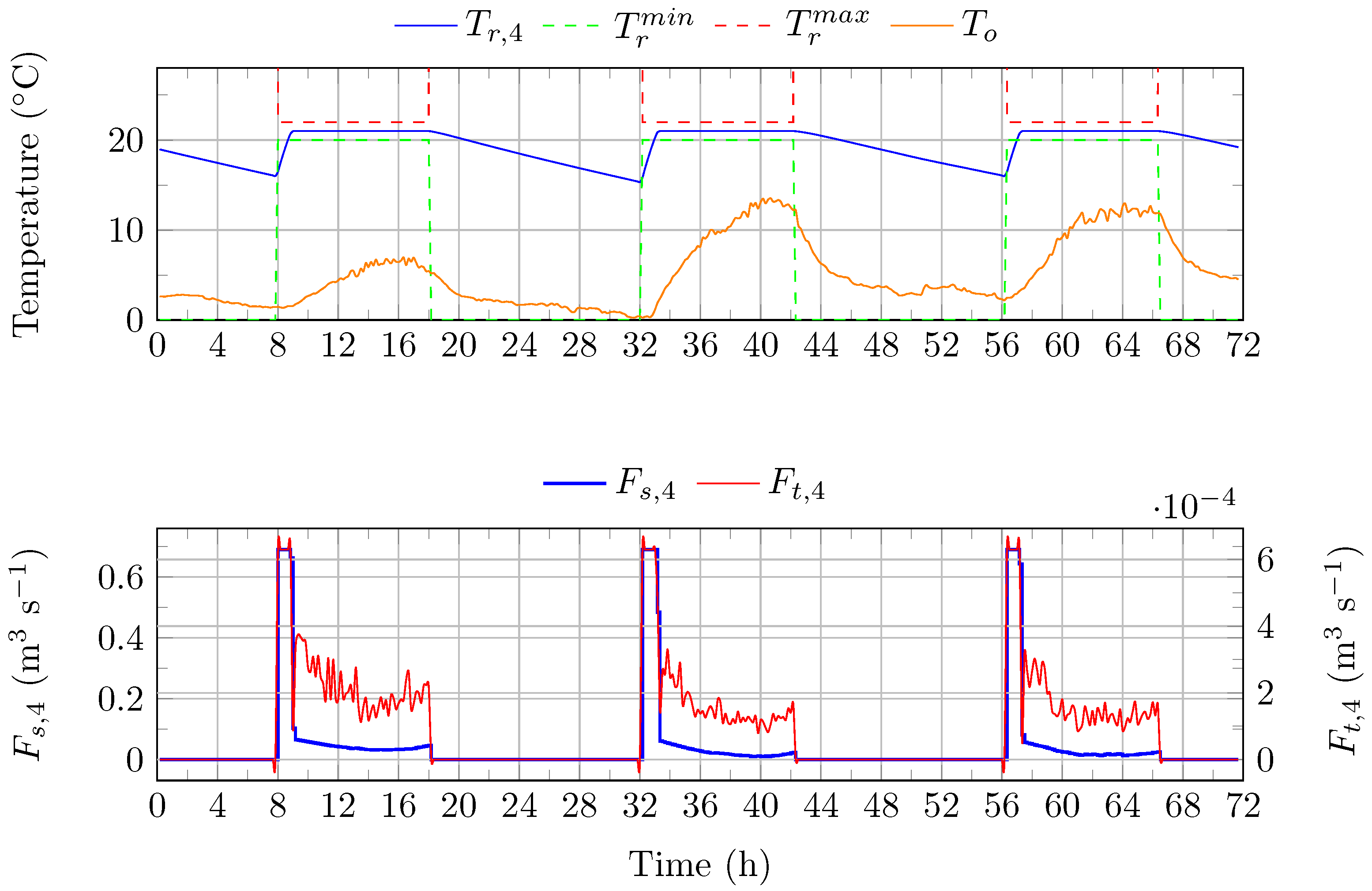
Table 1.
Modeling results. : air temperature in room z. : temperature of the water in the TES (layer j). RMSE: root-mean-square error. nRMSE: normalized root-mean-square error.
Table 1.
Modeling results. : air temperature in room z. : temperature of the water in the TES (layer j). RMSE: root-mean-square error. nRMSE: normalized root-mean-square error.
| Thermal Zones (R2, R3 and R4) | TES | |||||||
|---|---|---|---|---|---|---|---|---|
| February | May | May | ||||||
| RMSE | ||||||||
| nRMSE | ||||||||
Table 2.
PID controllers for the management of thermal comfort. TES: thermal energy storage. FCU: fan coil unit. : proportional gain. : integral gain. : derivative gain. N: filter coefficient.
Table 2.
PID controllers for the management of thermal comfort. TES: thermal energy storage. FCU: fan coil unit. : proportional gain. : integral gain. : derivative gain. N: filter coefficient.
| PID Controller | N | |||
|---|---|---|---|---|
| TES-FCU R1 | ||||
| TES-FCU R2 | ||||
| TES-FCU R3 | ||||
| TES-FCU R4 | ||||
| FCU R1/R2/R3 | ||||
| FCU R4 |
Table 3.
Simulation parameters.
| Room | R1 | R2 | R3 | R4 |
|---|---|---|---|---|
| Number of people | 1 | 1 | 4 | 16 |
| Beginning/end of the occupancy period | 8 AM/6 PM | |||
| Air temperature set point (occupancy/nonoccupancy period) | 21 /none | |||
| Minimum/maximum air temperature (occupancy period) | 20 /22 | |||
Table 4.
Air temperature constraint violation (3-day simulation). : PID-based strategy. : optimization-based MPC strategy. : optimization-free MPC strategy.
Table 4.
Air temperature constraint violation (3-day simulation). : PID-based strategy. : optimization-based MPC strategy. : optimization-free MPC strategy.
| [] | ||||
|---|---|---|---|---|
| Season | Strategy | R1/R2 | R3 | R4 |
| 0.20 | 0.05 | 0.66 | ||
| Winter | 0 | 0 | 0 | |
| 0 | 0 | 0 | ||
| 0.05 | 0.01 | 0.20 | ||
| Spring | 0 | 0 | 0 | |
| 0 | 0 | 0 | ||
Table 5.
Heat delivered by the FCUs (3-day simulation). : PID-based strategy. : optimization-based MPC strategy. : optimization-free MPC strategy.
Table 5.
Heat delivered by the FCUs (3-day simulation). : PID-based strategy. : optimization-based MPC strategy. : optimization-free MPC strategy.
| [kWh] | ||||
|---|---|---|---|---|
| Season | Strategy | R1/R2 | R3 | R4 |
| 2.2 | 2.2 | 15.6 | ||
| Winter | 1.5 | 1.3 | 11.4 | |
| 1.5 | 1.3 | 11.4 | ||
| 1.3 | 1.5 | 7.6 | ||
| Spring | 0.6 | 1.2 | 3.2 | |
| 0.6 | 1.2 | 3.2 | ||
Table 6.
Computational cost (3-day simulation). : PID-based strategy. : optimization-based MPC strategy (18 workers are used in parallel). : optimization-free MPC strategy. Calculation server used: two processors, Intel Xeon Gold 6230 @ 2.10 GHz with 20 cores and 40 threads, 512 Go of RAM, and an average CPU mark of 26,657.
| Computational Cost | ||||
|---|---|---|---|---|
| Season | Strategy | R1/R2 | R3 | R4 |
| 34 | 47 | 23 | ||
| Winter | 203,940 | 283,518 | 162,846 | |
| 5185 | 2754 | 2848 | ||
| 36 | 81 | 22 | ||
| Spring | 132,192 | 143,136 | 95,940 | |
| 2891 | 2827 | 3072 | ||
Table 7.
PID controllers for the management of thermal resources. SCs: solar collectors. HWT: hot water tank. HP: heat pump. : proportional gain. : integral gain. : derivative gain. N: filter coefficient.
Table 7.
PID controllers for the management of thermal resources. SCs: solar collectors. HWT: hot water tank. HP: heat pump. : proportional gain. : integral gain. : derivative gain. N: filter coefficient.
| System | N | |||
|---|---|---|---|---|
| SCs/HWT | ||||
| HP |
Table 8.
Electricity bought from the main grid (3-day simulation). : PID/rule-based strategy. : optimization-free MPC strategy. : optimization-based MPC strategy.
Table 8.
Electricity bought from the main grid (3-day simulation). : PID/rule-based strategy. : optimization-free MPC strategy. : optimization-based MPC strategy.
Electricity Bought from the Main Grid [ ] ] | |||
|---|---|---|---|
| Season | Strategy | No Use of PV Power Generation Surplus | Use of PV Power Generation Surplus |
| 26.36 | 21.91 | ||
| Winter | 14.08 | 12.34 | |
| 13.54 | 11.08 | ||
| 13.41 | 7.53 | ||
| Spring | 0.42 | 0.42 | |
| 0.31 | 0.35 | ||
Table 9.
emissions related to the electricity bought from the main grid (3-day simulation). : PID/rule-based strategy. : optimization-free MPC strategy. : optimization-based MPC strategy.
Table 9.
emissions related to the electricity bought from the main grid (3-day simulation). : PID/rule-based strategy. : optimization-free MPC strategy. : optimization-based MPC strategy.
| Emissions [] | |||
|---|---|---|---|
| Season | Strategy | No Use of PV Power Generation Surplus | Use of PV Power Generation Surplus |
| 55.8 | 46.5 | ||
| Winter | 35.6 | 31.7 | |
| 32.3 | 27.8 | ||
| 25.9 | 14.4 | ||
| Spring | 0.9 | 0.9 | |
| 0.7 | 0.7 | ||
Table 10.
Hourly average temperature () constraint deviation (3-day simulation). : PID/rule-based strategy.
Table 10.
Hourly average temperature () constraint deviation (3-day simulation). : PID/rule-based strategy.
| [] | |||
|---|---|---|---|
| Season | Strategy | No Use of PV Power Generation Surplus | Use of PV Power Generation Surplus |
| Winter | 1.43 | 1.41 | |
| Spring | 0.19 | 0.06 | |
Table 11.
Objective function (3-day simulation). : PID/rule-based strategy. : optimization-free MPC strategy. : optimization-based MPC strategy.
Table 11.
Objective function (3-day simulation). : PID/rule-based strategy. : optimization-free MPC strategy. : optimization-based MPC strategy.
| Objective Function [] | |||
|---|---|---|---|
| Season | Strategy | No Use of PV Power Generation Surplus | Use of PV Power Generation Surplus |
| 1167.2 | 1080.1 | ||
| Winter | 252.7 | 222.0 | |
| 240.5 | 206.7 | ||
| 310.9 | 150.9 | ||
| Spring | 6.7 | 6.7 | |
| 4.9 | 5.5 | ||
Table 12.
Computational cost (3-day simulation). : PID/rule-based strategy. : optimization-free MPC strategy. : optimization-based MPC strategy. Calculation server used: two processors Intel Xeon Gold 6230 @ 2.10 GHz with 20 cores and 40 threads, 512 Go of RAM and an average CPU mark of 26,657. ★ 18 workers in the parallel pool.
| Computational Cost | |||
|---|---|---|---|
| Season | Strategy | No Use of PV Power Generation Surplus | Use of PV Power Generation Surplus |
| 126 | 179 | ||
| Winter | 2824 | 2566 | |
| 3,280,284 ★ | 3,229,758 ★ | ||
| 157 | 176 | ||
| Spring | 1950 | 2669 | |
| 2,788,524 ★ | 2,589,102 ★ | ||
Disclaimer/Publisher’s Note: The statements, opinions and data contained in all publications are solely those of the individual author(s) and contributor(s) and not of MDPI and/or the editor(s). MDPI and/or the editor(s) disclaim responsibility for any injury to people or property resulting from any ideas, methods, instructions or products referred to in the content. |
© 2024 by the authors. Licensee MDPI, Basel, Switzerland. This article is an open access article distributed under the terms and conditions of the Creative Commons Attribution (CC BY) license (https://creativecommons.org/licenses/by/4.0/).
Share and Cite
MDPI and ACS Style
Mannini, R.; Darure, T.; Eynard, J.; Grieu, S. Predictive Energy Management of a Building-Integrated Microgrid: A Case Study. Energies 2024, 17, 1355. https://doi.org/10.3390/en17061355
AMA Style
Mannini R, Darure T, Eynard J, Grieu S. Predictive Energy Management of a Building-Integrated Microgrid: A Case Study. Energies. 2024; 17(6):1355. https://doi.org/10.3390/en17061355
Chicago/Turabian StyleMannini, Romain, Tejaswinee Darure, Julien Eynard, and Stéphane Grieu. 2024. "Predictive Energy Management of a Building-Integrated Microgrid: A Case Study" Energies 17, no. 6: 1355. https://doi.org/10.3390/en17061355
Note that from the first issue of 2016, this journal uses article numbers instead of page numbers. See further details here.