
Empowering Active Users: A Case Study with Economic Analysis of the Electric Energy Cost Calculation Post-Net-Metering Abolition in Slovenia

Faculty of Electrical Engineering and Computer Science, University of Maribor, 2000 Maribor, Slovenia
*
Author to whom correspondence should be addressed.
Energies 2024, 17(6), 1501; https://doi.org/10.3390/en17061501
Submission received: 26 February 2024
/
Revised: 15 March 2024
/
Accepted: 18 March 2024
/
Published: 21 March 2024
(This article belongs to the Special Issue Climate Changes and the Impacts on Power and Energy Systems)
Abstract
:This paper addresses the issue of the abolition of annual net metering in Slovenia and compares the electric energy costs for the studied active user after the abolition. The article also provides an exploration of the role played by an aggregator, which serves as a central entity that enables individuals to participate in the electric energy market. An analysis of the case study of an active user was made, where an analysis was made of the measurements of household consumption and photovoltaic plant production for the year 2022. This article presents an economic analysis with and without net metering and an analysis of the aggregator involvement strategies. In addition, a battery energy storage system was also considered in the analysis. An important part of the article is the identification of the flexibility potential for shiftable loads, which enable an aggregator to acquire insight into the energy consumption profile and energy production profile of active users. The following indicators were used to compare the strategies: annual electric energy cost and the indicators including self-sufficiency, self-consumption, and grid dependency. The findings indicate that, even in the absence of annual net metering, the active user can lower their costs for electric energy with the help of an aggregator.
1. Introduction
The flexibility potential of active users is ever increasing due to the growth in the use of the following power-consuming and/or power-producing appliances in households: heat pumps (HPs) for heating, electric vehicles (EVs), battery energy storage systems (BESSs), and renewable energy sources (RESs) such as solar power plants. An active user is an individual or a group of end-users who provide services for adjusting consumption and/or production. The integration of home appliances with home energy management systems (HEMSs) does present some challenges for households due to the complexity of the underlying processes and technologies [1,2], but also helps to improve the energy efficiency in households. The lack of awareness among active users about the sustainable use of electric energy decelerates the usage of HEMSs in households [3].
The EU countries have a variety of programs to encourage households to install photovoltaic systems (PVs) in their homes, as discussed in [4,5,6]. One of the programs that encourage households to install PV plants in Slovenia is net metering, which is described later. In [7], a method for the sizing of a PV plant and the environmental perspective are presented for a case study in Slovenia. The support laws and regulations of countries that encourage PV plants are some of the key factors in the economic feasibility of investing in a PV plant. An overview of the supporting policies in five EU countries through investment profitability is provided in [8]. This paper offers a detailed analysis of the support policies for photovoltaic installations in the residential sector across major European markets such as Flanders (Belgium), Germany, Italy, Spain, and France. It evaluates the economic viability of a household investment in a photovoltaic installation through a model based on the discounted cash flows of the installation over its lifetime. The study suggests that Italy’s support system has been the most profitable among the countries studied since 2010. Despite decreasing support levels, residential installations are still profitable in most cases under the current support policies, except for Spain. The study further highlights the potential of self-consumption to increase profits, especially in Spain and Germany. However, Flanders’ policy has no impact on levels of self-consumption. Finally, a comparison of past and present policies indicates varying levels of success in keeping the profitability of investments stable over the years, depending on the efficiency of the support policy. Germany’s support system stands out as the most balanced one over the last five years. The results of the study show that the supporting policies have a significant impact on investments’ profitability. Household users can also sell their electric energy and have different options, as discussed in [9], which compares the following three electric energy sales mechanisms: feed-in tariffs, net metering, and net purchase with sale. Each mechanism has been described using a simple microeconomic model. The mechanisms have been compared in terms of social welfare and the retail electric energy rate.
Annual net metering allows the solar power plant to cover the household’s electric energy needs while surpluses and deficits are regulated by the grid. When production exceeds consumption, the power plant sends the excess energy to the grid, while, during lower production time, the household receives electric energy from the grid. The annual calculation is made only once a year, at the end of the calendar year, and is based on the difference between the supplied and received electric energy. The decision as to whether any excess energy that arises after the end of the billing period will be handed over to the supplier for a fee or free of charge is a matter of agreement between the customer and the supplier. Several studies have been performed to optimize the size and operation of PV plants. In [10], the researchers were focused on the optimal design of PV systems in light of the specificity of Polish regulations. Since the annual net metering was valid, the annual consumption was relevant in the dimensioning of the PV plant. With the abolition of net metering, the methods for sizing PV plants will change.
The Directive 2019/944 EU [11] requires that the network fee must be non-discriminatory, regardless of whether the household user is included in the net metering policy. With the new regulation, the household user will be required to pay a network fee for all the electric energy delivered from the distribution grid [12]. Therefore, Slovenia coordinated its legalization with the EU legislation and adopted the Act on Promoting the Use of renewable energy sources [13] and the regulation on self-supply with electric energy from renewable energy sources [14], which will enter into force in 2024. Legislations will bring major changes in Slovenia’s network fee tariffs and abolish the concept of annual net metering, and cause many households in Slovenia to wonder about the profitability of investments in a PV plant. Households with installed PV plants need to consider their energy management strategies.
There is always a discrepancy between produced energy and household consumption. Therefore, for a reliable power supply, it is essential to connect the PV plant to the distribution grid or energy storage system. With the development and massive integration of BESS, many studies have been conducted to address the advantages of BESS in PV applications. A study performed by [15] is being carried out to provide household and commercial users with the optimal size of a PV plant based on their yearly consumption. In [16], the researchers proposed a multi-objective optimal sizing of a grid-connected household with a PV plant and BESS to minimize the total electric energy cost and grid dependency. In [17], the optimal size for a PV-BESS system is considered by the depth of discharge value and the optimal tilt angle of the PV panels. The BESS degradation was ignored. In [18], a framework is presented of a two-stage optimization model for the planning and operation for a household with a PV-BESS system. As a result, it is necessary to choose the optimal size of the PV and BESS to achieve the minimum cost of the system.
Active users can vary their electric energy consumption according to their needs and preferences, taking advantage of dynamic pricing and generation from renewable energy sources. Price-based programs are based on dynamic tariffs, where the prices of the tariff values change depending on the electric energy market circumstances and network conditions. Price-based programs based on time and power demand can be classified as the following [19]: time-of-use pricing, real-time pricing, and critical-peak pricing. In [20], a self-scheduling model for a HEMS is presented considering time-of-use pricing and real-time pricing, aiming to reduce the users’ electric energy costs. Additionally, various scenarios with the inclusion of BESSs are studied, to examine their impact on optimal performance. A HEMS optimization model for scheduling home appliances effectively under a time-of-use pricing tariff is presented in [21]. The HEMS optimizes the performance of multiple household appliances, including BESSs, EVs, air conditioners, and water heaters, to minimize electric energy costs.
The HEMS allows active users to manage their consumption and/or production actively, and to participate in new energy services and new opportunities in flexibility markets [22,23]. New energy services are implemented by combining consumers and producers. A more active involvement of active users will also require a new concept of the flexibility market. In [24], the trends in the new flexibility market were selected and compared, where the results showed that the new market platforms present promising models regarding technical and economic justification. Aggregator platforms for local trading between active users, like promoting peer-to-peer trading, were also analyzed in the article.
Demand-side flexibility (DSF) mechanisms can be classified into implicit and explicit DSF mechanisms [25]. Under the implicit DSF mechanism, active users increase or decrease consumption or production in response to electric energy price signals. Under the explicit DSF mechanism, active users increase or decrease consumption or production in response to the aggregator signal, which is based on energy market needs and ancillary products. The aggregator is a retailer of flexibility and has different roles: they aggregate, and coordinate flexibility provided by users, trade with flexibility, and conclude contracts with active user and flexible users (Flex Requesting parties), the transmission system operator, the distribution system operator, and the balance responsible party (BRP). In response, new aggregator platforms and flexibility market models are being developed and analyzed in [24]. The regulatory framework for the aggregator role is still under discussion, and is implemented differently in several EU countries. The status of explicit DSF for active users in the 26 EU Member States was examined in [26].
Consumption in households consists of different types of power-consuming appliances. In [27], home appliances are categorized as shiftable, interruptible, weather-based, and non-manageable. Shiftable appliances have flexible delays with specific energy consumption profiles, e.g., washing machines, dishwashers, etc. Interruptible appliances have fixed energy consumption when they are switched on and non-energy consumption when they are switched off, e.g., water heaters, refrigerators, etc. Weather-based appliances depend upon the weather and dimensions of the premises, e.g., heating, ventilation, and air conditioning appliances. Non-manageable appliances do not have the option to adjust their consumption, e.g., TVs, lights, etc. The home appliances in [28] are divided into two groups, shiftable and non-shiftable, and this division of home appliances is used in the following.
The HEMS requires the development of a framework for handling the energy needs and demands of an active user without compromising the comfort level and without greater involvement of the active user, so the process must be as automated as possible. The increasing use of RESs and BESSs in households can have significant benefits to the operations of HEMSs. The advantage of using a BESS is to store produced energy with the RES, and to use energy when the electric energy price is high. In [29], a HEMS with a RES and BESS is presented, where the findings obtained by simulating the problem using household data thoroughly confirm the efficiency of the provided HEMS in lowering the electric energy cost while keeping the appropriate level of consumer discomfort.
This work aims to examine the possibilities for an active user after the abolition of net metering and explore the economic analysis of households with solar PV plants in Slovenia, comparing the cost-effectiveness of households with and without net metering policies. An integral aspect of the article involves calculating the flexibility potential of an active user, which is technologically available using algorithms for detecting flexible loads. The focus is on a case study of a single-family home with an installed PV plant. In the study, a comprehensive analysis is carried out with and in the absence of net metering, as well as investigating strategies with aggregator involvement. The self-sufficiency indicator (SS), self-consumption (SC) indicator, grid-dependency indicator (GD), and annual electric energy costs (PEB) are calculated to determine the economic viability of each strategy. Two main contributions are provided in this work. Firstly, the identification algorithms for identifying shiftable loads are included, which offers a robust methodology for the recognition of such loads. Secondly, it presents an analysis encompassing scenarios with and without net metering alongside strategies involving aggregators.
The paper is organized as follows. An introduction to the discussed problem is given in the first section. The case methodology is discussed in the second section. In the third section, a case study description is presented, whereas the fourth section presents and discusses the obtained results. The fifth section gives a conclusion, where the outline is presented for future work.
2. Methodology
2.1. Electric Energy Cost Calculation Model
Understanding the electric energy cost can help active users to make informed decisions about their energy consumption and to optimize their energy use to reduce costs. Electric energy costs consist of the following: the market price of electric energy, the network charge (transmission network charge and distribution network charge), contributions (a contribution for a market operator (C1), a contribution for energy efficiency (C2), a contribution to support the production of electric energy from renewable energy sources (RES), and high-efficiency co/generations (C3)), and the excise duties on electric energy (C4). The network charge represents the amount that an active user of the transmission system must pay for utilizing the system. Its purpose is to cover the costs incurred by the electricity system operators in each year of the regulatory period. The Energy Agency establishes the network charge for the electricity system in accordance with the Legal Act on the methodology for determining the regulatory framework for electricity system operators. The prices set by the Energy Agency for contributions and charges, which were valid in 2022, were used. In Slovenia, there is a two-rate tariff system, which is shown Figure 1. The low tariff (LT) is applied during off-peak hours, which last from 00:00 to 5:59 and from 22:00 to 23:59. The LT is also used on holidays and weekends. The high tariff (HT) is applied during peak hours, which last from 6:00 to 21:59.
The prices for LT (PLT) and price HT (PHT) are shown in Table 1. The network charge for LT (NCLT) is lower than the network charge for HT (NCHT). The capacity charge (CC) is a fixed charge based on the contracted capacity of the discussed household user. The capacity charge must be paid monthly. The rated power is determined by the current limiter, while the connection power and billing power are determined by the network regulation. The billing power (PB) of the user is determined by the contract with the user based on the network regulation, according to which the billing power may also be lower or higher than the connection power. The billing power determines the amount of two charges on the electric energy bill: CC and C3. The CC and C3 factors are paid monthly and are not related to the electric energy consumption, but rather to the contracted power. Table 1 presents prices for tariffs and different charges for calculating the final price of electric energy without VAT.
The annual electric energy costs (PE) for a user are calculated using Equation (1), where factor 12 is used for the CC and C3 factors because we are calculating the consumption for the whole year. To allocate to the different tariff rates accurately, it is necessary to segregate the total load consumption based on the time of the day. The data were divided into corresponding periods to determine the energy consumption under LT () and HT (), and can be written by (1).
2.2. Calculation of the SS, SC, and GD Indicators
The self-sufficiency (SS), self-consumption (SC), the grid-dependency (GD) indicators are calculated and can be used to assess the level of energy independence of a system. The SS indicator is used to estimate how much energy a PV plant can provide for its own needs without relying on external resources. The SS indicator describes the relationship between the energy produced from the PV plant for the observed time period and the total consumption of the household for an observed time period, and can be calculated using (3). The observed time period (T) can be a day, a month, a year, or any period of time.
The SC indicator is used to estimate how much electric energy generated from the PV plant is actually used in a 15 min time interval. The SC indicator describes the relationships between the energy actually consumed from the PV plant for the observed time period and the total consumption of the load for the observed time period, and can be written by (4).
When the BESS is included in the household, the SC indicator is used to estimate how much electric energy is generated from the PV plant, and the BESS is actually used in a 15 min time interval. Equation (5) is used to calculate the SC indicator with the inclusion of the BESS in the household.
The difference between the SS in the SC indicators is that the SS indicator is used to calculate a ratio between the total energy produced from the PV plant and the total consumption of load for the observed time. The SC indicator is used to calculate how much energy produced electric energy from a PV plant is actually consumed in a 15 min interval by a household user. The GD indicator is used to estimate the level of grid dependency. It is defined by (6) and describes the ratio between the consumption from the grid and the total load consumption.
The mentioned parameters, particularly the SS and GD indicators, assume a crucial role under the new accounting system, as the network no longer serves as virtual storage for produced energy. In ideal scenarios, our goal is absolute independence from the grid (SS = 100%). However, achieving this would necessitate an economically unjustifiably large BESS capable of maintaining such autonomy, especially during the winter months. Conversely, we aim to minimize the GD indicator, implying a shift in the load profile. Active users are encouraged to align their consumption with daily production, thereby reducing the GD indicator. Both parameters, therefore, wield significant influence in the decision-making process for individuals when determining the placement of the RES and BESS.
2.3. Description of the Aggregator Role
Household consumers and active users are becoming more equipped (PV plants and advanced metering) and have the potential to provide new services of flexibility. Flexibility is described as a movement in the active user’s load profile caused by changes in the load profile. Although the flexibility potential of household active users is limited, an effective grouping of active users may be sufficient to keep the power system balanced. A new role—the aggregator—is required in the energy value chain for the consumers and prosumers to have access to this flexibility market. The aggregator connects numerous modest flexibility resources into a usable flexibility volume by working between active suppliers and active users. With the participation of active users in the energy value chain, an understanding of new relationships, services, and programs will be required. Any legal or natural person who wishes to participate actively in the electric energy market will have to join the Balance Scheme. Balance Schemes and electric energy market operators are connected through a set of procedures, regulations, and market mechanisms that ensure an efficient and reliable supply of electric energy. This connection is critical for maintaining the balance between electric energy generation and consumption in the power grid. The electric energy market in Slovenia is organized hierarchically into a Balance Scheme, which is managed by the electric energy market operator, Borzen, and d.o.o.
Document [30] addresses several possible aggregator implementation models that can be used to implement the aggregator role in current energy markets. The document presents six aggregator models, and one of these models was adopted for further research. The relationships between an active user, a new entity in the future electric energy market aggregator, and supplier are shown in Figure 2. The aggregator establishes all the contractual relations necessary to participate in the flexibility market and establishes connections with customers who own flexible resources. Active users will be compensated according to the degree of asset flexibility they provide. In order to adhere to the size and temporal requirements of particular flexibility products, the aggregator constructs a portfolio of assets. A balance responsible party (BRP) is in charge of balancing demand and supply actively for its portfolio. The aggregator is in charge of activating flexibility, while the active user is in charge of energy change. It is important to emphasize that, in order to participate in market mechanisms where active users can offer their flexibility potential, the active user must/can have separate contracts with the electric energy supplier and the aggregator. Aggregators empower active users to participate actively in DSF mechanisms to obtain incentives to reduce the load during peak periods. It is crucial to emphasize that aggregators play a key role in optimizing energy consumption. By managing and coordinating the various resources in their portfolios actively, aggregators can help active users implement energy conservation strategies, demand response initiatives, and redeployment practices.
Electric energy trading involves buying and selling electric energy in various forms, such as power contracts, futures, options, and swaps. This trading can occur between different market participants, including active users, aggregators, and energy service providers. Electric energy markets are structured differently in different regions and countries, but they all aim to provide an efficient and reliable electric energy supply at a reasonable price. Generally, electric energy markets operate based on supply and demand, where the price is set by the intersection of the supply curve (i.e., the amount of electric energy producers are willing to generate at a given price) and the demand curve (i.e., the amount of electric energy consumers are willing to buy at a given price).
Electric energy trading can occur in various markets, including wholesale markets, balancing markets, capacity markets, and futures markets. Wholesale markets are used for large-scale transactions between electric energy producers and consumers, while spot markets allow for the real-time trading of electric energy at current prices. Futures markets allow market participants to trade contracts for the future delivery of electric energy.
An electric energy market model requires crucial data from previous trading periods. Patterns and trends in electric energy demand and supply, as well as the prices at which electric energy is traded on the market, can be identified by analyzing the data. This information can then be utilized to develop a model that simulates the behavior of the electric energy market under different conditions. Energy exchanges such as the BSP South Pool Energy Exchange serve as an important source of data for data acquisition. The BSP South Pool Energy Exchange allows electric energy trading in the Slovenian and Serbian electric energy on the day-ahead, intraday, and balancing markets. Furthermore, the BSP Energy Exchange offers various other services and products, such as capacity reserve auctions, balancing market services, and the trading of guarantees of origin certificates. These products and services aim to provide a comprehensive platform for market participants to manage their electric energy portfolios and risks efficiently. BSP stands for the “BSP Regional Energy Exchange”, which is a Slovenian energy exchange company that operates a trading platform for trading electric energy. A market model for electric energy trading was developed based on day-ahead trading annual data. The hourly trading price (Tp) data were employed in our analysis. This information was used to develop a model that simulates the behavior of the day-ahead electric energy market. Figure 3 offers a detailed overview of the hourly trading price fluctuations that occurred throughout 2022.
The patterns in the prices at which electric energy is traded on the day-ahead market were identified by analyzing the data. The analysis of the trading price on the day-ahead market revealed that the peak trading price of electric energy on the day-ahead market was observed in August, while the minimum trading price of electric energy on the day-ahead market was noted in December.
2.4. Identification of Flexibility Potential for a Shiftable Load
By defining the flexibility potential, an active user’s appliances and sources can be utilized optimally. This enables the aggregator to gain insight into the active user’s energy consumption profile and energy production profiles. The ability of an active user to consume or produce electric energy in response to an external signal is referred to as positive and negative flexibility. The positive flexibility potential represents the capability to increase energy consumption or decrease electric energy production as needed. The negative flexibility potential relies on the ability to decrease electric energy consumption or increase electric energy production as needed. Both types of flexibility potential are crucial and can be offered to an aggregator. The flexibility potential of the active user is determined by evaluating the flexibility potential for each shiftable household load. Shifting the active user’s appliances and sources can help reduce the cost of electric energy. However, these changes require some level of compromise in terms of daily electricity pattern usage routines. This compromise can result in discomfort, which can be defined as a loss or impairment of energy comfort. The literature has identified three types of discomfort that have been discussed in this context [31]: delay or waiting time due to shifting time-flexible appliances, temperature deviation due to thermostat settings of temperature-based appliances, and power deviation resulting from reduced power of instant power-based appliances. To ensure the active user’s comfort in strategy 2, a strategy was implemented where shiftable loads were manipulated only once a day, with each activation lasting just 30 min. The approach aimed to minimize the active user’s discomfort while still achieving a reduction in cost for electric energy.
The flexibility potential of EVs is defined by the EV charging habits that are analyzed throughout the year. The flexibility potential of EVs is defined with (7), where is the electric energy consumption of the EV. The assumptions considered in defining the flexibility potential of the EV are as follows: the EV is charged every day and the EV is available every day after 16:00. The positive flexibility potential of the EV is defined by allowing the reduction and rescheduling of EV charging during charging periods, and changing the positive flexibility potential on an annual basis, as can be seen in Figure 4a. The negative flexibility potential of the EV includes identifying instances when the EV has not yet been fully charged within the day, and if it is past 16:00, the charging can be rescheduled. The negative flexibility potential of the EV throughout the year can be seen in Figure 4b.
The flexibility potential of the HP is defined by (8), where is the electric energy consumption of the HP. The negative flexibility potential of the HP on an annual basis can be seen in Figure 4b, while the positive flexibility potential of the HP on an annual basis can be seen in Figure 4d. The fHP weighting factor is a parameter that typically ranges between 0 and 1, determining the degree to which we want to adjust the power of the HP.
The flexibility potential of the PV is defined with (9), where is the electric energy produced from the PV and is the consumption of the load. The negative flexibility potential of the PV size is defined as the difference between the energy produced from the PV and the consumed energy, and can be seen in Figure 5a. The positive flexibility potential of the PV is defined as zero, because PV plant systems are dependent on solar irradiance, which cannot be controlled by an active user, and can be seen in Figure 5b. The amount of produced energy from the PV plant is determined primarily by the environmental conditions.
The flexibility potential of a BESS can be quantified based on its capacity to store and release energy at specific times, its efficiency in these processes, and its ability to respond to various grid events and signals. The operation and dynamics of the charging and discharging of the BESS are different for different strategies, which are described below. The flexibility potential of the BESS is defined by (10), where SOCmin and SOCmax are changing according to the strategy and different modes. The flexibility potential of the BESS is offered to an aggregator only in strategy 2. The negative flexibility potential of the BESS on an annual basis can be seen in Figure 5c, while the positive flexibility potential of the BESS on an annual basis can be seen in Figure 5d.
2.5. Definition of Strategies
The research aims to explore the possibilities for active users after the abolition of net metering, and two strategies were designed for this purpose. Engaging in the electric energy market is a viable option for an active user. Nonetheless, since direct participation in the electric energy market is not possible, the active user needs to establish a connection with an aggregator. Two strategies were formulated to evaluate the advantages for an active user in collaborating with an aggregator. Given the recent approval of subsidies by the state for the construction of a BESS, there has been a notable increase in their adoption in households. Consequently, the upcoming analysis focuses on testing the strategy on two active user cases: one with the PV plant and another with both the PV plant and BESS. The operation for strategy 1 involves offering only excess energy from the PV plant to the aggregator. Strategy 2 offers a shiftable household load in addition to excess energy from the PV plant to the aggregator.
2.5.1. Strategies for an Active User with a PV Plant Only
In Figure 6a, the presentation shows strategy 1, which shows the scenario where the engaged active user provided excess energy from the PV plant to the aggregator. In Figure 6b, the presentation shows strategy 2, which shows the scenario where the engaged active user provided excess energy from the PV plant and shiftable load to the aggregator. Shiftable loads in strategy 2 are identified using the identification algorithm for shiftable loads presented in Section 2.3. Strategy 2 offers the flexibility potential of the HP and the flexibility potential of the EV to an aggregator. By incorporating shiftable loads, the active user’s flexibility potential can be increased, providing the aggregator with more flexibility potential.
Operation during strategy 1 for an active user with a PV plant only: The electric energy produced from the PV plant () is divided into two energies: the energy consumed directly by the load () and the excess energy () which is offered to an aggregator, and, further, to the electric energy market, and can be written with (11).
The load consumption is equal to the energy taken from the grid () and the energy produced with the PV plant that is actually consumed directly by the load (), and can be written by (12).
In strategy 2, the following three modes of operation are distinguished: operation before activation, operation during activation, and operation after activation. Operation during activation is the same as in strategy 1, as the active user’s flexibility potential is offered to an aggregator. Operation before and after activation will be presented in the following. The energy produced from the PV plant () is divided into the following two energies: the energy that supplies the load directly () and the excess energy () which is sent to the grid, and can be written by (13). The distribution of the load consumption () remains the same as in (13).
2.5.2. Strategies for an Active User with a PV and BESS
In Figure 7a, the presentation shows strategy 1, which shows the scenario where the engaged active user provided excess energy from the PV plant that remained after charging the BESS to the aggregator. In Figure 7b, the presentation shows strategy 2, which shows the scenario where the engaged active user provided excess energy from the PV plant, BESS, and shiftable load to the aggregator. The shiftable loads in strategy 2 are identified the same as in the previous example.
Operation during strategy 1 for an active user with a PV and BESS: the energy produced from the PV plant () is divided into the following two energies: the energy that supplies the load directly () and the excess energy () which is offered to an aggregator, and can be written by (14).
The load consumption () is equal to the energy taken from the grid () and the energy produced with the PV plant that is actually consumed directly by the load (), and can be written by (15).
Excess energy from the PV plant is equal to the energy sent to the aggregator () and the energy that charges the BESS ().
Three modes of operation are discussed for operation during strategy 2 for an active user with a PV and BESS. The operation before and after activation will be presented in the following. The energy produced from the PV plant () is divided into two energies: the energy that supplies the load directly () and the excess energy () which is offered to an aggregator, and can be written by (17). The distribution of the load consumption () remains the same as in (15).
The excess energy from the PV plant is equal to the energy sent to the aggregator () and the energy that charges the BESS ().
Operation of the BESS during strategy 1: The efficiency of charging () and discharging () are considered when energy is stored in the BESS. The BESS is charged when there is excess energy available. The energy stored in the BESS () is positive in the case of charging the BEES, and is calculated according to (19).
Discharge begins when the energy from the PV plant is not sufficient to consume the load. is negative in the case of discharging the BEES and is calculated according to (20).
The energy stored in the BESS is calculated using (21), where is the energy stored at the previous moment and the .
The state of charge (SOC) is the ratio between the energy stored in the BESS and the size of the BESS, and is calculated using (22).
The operation of the BESS during strategy 1 can be described using (23), and operates between the lower limit (SOCmin), which is 20%, and the upper limit (SOCmax), which is 90%.
2.5.3. Elaboration on the Distinction in the Operation of the BESS between Strategy 1 and Strategy 2
In strategy 1, the BESS operates within the range of the lower limit of the SOCmin set to 20% and the upper limit of the SOCmax set to 90%, as shown in Figure 8a. The operation of the BESS in strategy 2 is divided into the following 3 modes: before the operation, during the operation, and after the operation of the BESS. Before the activation, the SOCmax is set to 60%, as seen in Figure 8b. Therefore, the BESS remains available for charging or discharging during the activation mode. During the activation, the BESS undergoes charging or discharging based on the aggregator signal. The BESS is operated during the activation within the range of the lower limit of the SOCmin set to 10% and the upper limit of the SOCmax set to 90%. After the activation mode, two cases can be distinguished based on the action during activation. The BESS was discharged when a signal for negative flexibility was received from the aggregator. Subsequently, after the activation, the BESS underwent recharging from the grid. In a case where a signal for positive flexibility was received from the aggregator, and the BESS was charged from the grid; subsequently, after the activation, the BESS underwent discharging to the grid. A more detailed presentation of the BESS performance during and after activation will be elucidated in the Results section.
2.6. Profit Determination
The profit from the sale of excess energy from the PV plant, PPV_e is calculated using (24), where is the excess energy from the PV plant, Tp is the trading price, and fA is a weighting factor that indicates how much the aggregator reduces profit relative to the Tp. Factor fA is in the range of 0 to 1. If factor fA is equal to 1, it signifies that the aggregator compensates in alignment with the prevailing electric energy prices on the day-ahead market.
The difference between the electric energy payment PEB and the profit from the sale of excess energy PPV_e is calculated using (25), which is represented as Pd. Pd signifies the actual costs for electric energy that the active user is obligated to pay subsequent to the sale of excess energy.
3. Case Study Description
The case study involved an active user in a single house with an installed PV plant of 11 kW. The house was equipped with an HP for central heating and a charging station for an EV. The research process consisted of several critical stages, as shown in Figure 9, starting with data acquisition. Information on electric energy consumption and energy produced from the PV plant in the 15 min interval was obtained on the “Moj elektro” platform. The data from the platform were exported in Excel and processed further in Matlab. The next step was data analysis, focusing on the consumption and production patterns. Following that, the identification of shiftable loads was conducted, and, additionally, a BESS was included. Important data-driven results were derived as a result of this comprehensive analysis. The results were divided into the following 3 categories: the analysis with net metering, the analysis without net metering, and the analysis to evaluate the advantages of a collaboration between an active user and an aggregator, where two strategies were tested.
3.1. Analyzing the Data
The analysis was conducted by examining the daily energy consumption and PV plant production records from the previous years. An analysis was carried out of the active user electric energy consumption and PV production for the year 2022. The daily of each month is presented in Figure 10a. It can be seen how changed depending on the season. The average daily was 31.26 kWh, with a total yearly of 11.17 MWh. In Figure 10b, the average of each month is presented, with higher production during the summer months. The average daily was 29.81 kWh, with a total yearly of 11.97 MWh. Based on the data, it can be inferred that the winter consumption is higher than the summer consumption due to the use of an HP for heating. Additionally, PV production is at its peak during the summer and at its lowest during the winter.
3.2. Algorithm for Shiftable Load Identification
Active users must estimate their flexibility potential to provide flexibility services. The identification of flexible loads in an active user profile is key in the estimation of the flexibility potential. It is also necessary to determine the degree of flexibility of the associated loads with a weighting factor. The algorithm for the identification of the EV and HP is presented below. The Algorithm 1: Identification of EV is designed to identify the moment with the highest electric energy consumption within each day. After the moment with the highest consumption is identified, the consumption for four moments before and after are examined to determine the EV consumption.
| Algorithm 1: Identification of EV | ||
| Load input parameter () | ||
| for t = 1,..,tend(365) → days in year | ||
| if t== tLT → max for that day | ||
| → find max consumption and index for that moment for every day | ||
| End | ||
| calculate the consumption of EV if | ||
| calculate the consumption of EV | ||
| is a vector of EV consumption for every 15 min for a whole year | ||
The Algorithm 2: Identification of HP was designed to compare the consumption between summer and winter days. The first step is to deduct the consumption of the EV from the total consumption. The average consumption for the summer dates is calculated next. Then, the algorithm subtracts the average summer consumption from the consumption in the heating season to determine the HP consumption. The summer season was defined from 21 June 2022 to 23 September 2022 and the heating season was defined from 1 January 2022 to 10 March 2022 and from 1 October 2022 to 31 December 2022.
| Algorithm 2: Identification of HP | |||
| Load input parameter () | |||
| →EV consumption is subtracted from the consumption of all loads | |||
| Find summer dates (21 June 2022 till 23 September 2022)→ | |||
| For t = | |||
| = mean()→average summer profile for every 15 min | |||
| End | |||
| Find dates for the heating season (21 June 2022 till 23 September 2022) → | |||
| for t = 1,..,thd → days in year | |||
| End | |||
| calculate consumption of HP | |||
| is a vector of EV consumption for every 15 min for a whole year | |||
The results of the algorithm for the identification of shiftable loads are presented in Figure 11, providing a comprehensive overview of the energy consumption patterns. The results of the EV recognition algorithm can be observed in Figure 11a,c. The highest point of total consumption during the day was located and is marked in Figure 11a,c with a gray dashed line. There is no noticeable difference between the EV consumption during the summer months in Figure 11a and the winter months in Figure 11c. The performance of the HP recognition algorithm is observed in Figure 11b,d. On the selected summer day, there was no HP consumption, while, on the selected winter day, the HP consumption was detected.
With the help of the identification algorithms, the consumption was divided into the following three categories: EV consumption and HP consumption, which both can be referred to as the consumption of shiftable loads and non-shiftable loads, as seen in Figure 12, where the consumption is presented for each month. The annual consumption of the EV amounted to 2 MWh, with the electric energy consumption remaining relatively consistent throughout the year, with a slight increase during the winter months due to the cold weather impacting to the travel range of the EV. The annual consumption of the HP amounted to 3 MWh, while the annual consumption of the non-shiftable household load amounted to 6 MWh.
4. Results and Discussion
4.1. Analysis with Net Metering
The analysis carried out using net metering revealed that the active user involved in net metering only has to pay the difference between the consumed and produced electric energy if the user consumed more energy than produced. Based on the analyzed data, the annual load consumption of was 11.17 MWh, while the energy produced from the PV was 11.97 MWh. Since the active user produced as much energy as they consumed, they only needed to pay the monthly fixed fees, which include the capacity charge and contribution C3. As a result, the active user involved in net metering paid EUR 96.07 without VAT for PE, which is calculated using (26).
Despite its proven benefits, the net metering policy in Slovenia is set to be abolished. This upcoming change is expected to transform the financial landscape for active users. As a result, it has become crucial to evaluate the economic feasibility of PV plants in the absence of net metering and explore the benefits of the active user’s collaboration with an aggregator, where two strategies were investigated.
4.2. Analysis without Net Metering
With the upcoming abolition of net metering, the active user will no longer be enrolled in the net metering policy, which means that annual accounting will no longer be available. Therefore, an analysis of the consumed and produced energy was conducted in 15 min time intervals without net metering, which yielded the results shown in Table 2. The analysis of 15 min time intervals showed that the was only 1.92 MWh, which means that minimal electric energy was consumed in the 15 min interval. Without involvement in the net metering policy, the active user with a PV plant would only have to pay EUR 1401.2 for the PEB, and the PPV_e would be EUR 0, which means the Pd would be EUR 1401.2.
The grid is often perceived as a vast storage system due to the implementation of net metering policies. However, this perception fails to acknowledge the inherent limitations of the grid in storing excess energy generated by PV plants effectively, particularly during peak production periods in the summer. As a result, mismatches between energy production and consumption arise, notably during the winter months, when the demand escalates due to increased use of heat pumps for heating purposes. Such discrepancies pose challenges to system stability. This article has introduced indicators such as SS, GD, and SC to provide a more accurate representation of the level of self-sufficiency exhibited by active users and their dependence on the power grid. The SS indicator was 107%, indicating that the PV plant produces more electric energy annually than the active user consumes. However, only 17% of the electric energy produced by the PV plant was consumed, resulting in an SC indicator of 17%. The GD indicator was 83%, indicating that the majority of the electric energy consumed was from the grid. The GD indicator was very high because the produced energy from the PV was not consumed at the same 15 min interval. In the absence of net metering, the results of the indicators remained unchanged when compared to the results obtained through strategy 1. Therefore, no distinct outcomes were mentioned for strategy 1. Figure 13a–c represent the variations in the SS, GD, and SC indicators over the entire year. The SS indicator was highest in the summer months, where the values reached up to 300%, which means that the PV plant produced more electric energy than the active user consumed. However, in the winter months, particularly in January and December, the amount of the SS indicator decreased drastically to 20%, which was the lowest point throughout the year. The GD indicator was higher in the winter months and lower in the summer months, while the SC indicator was lower in the summer months and higher in the winter months. In the month of August, the SS indicator showed that the active user had produced more electric energy than they had consumed, with a percentage of 300%. However, taking a closer look at the GD indicator for the same month, it was observed that it was only 67%, while the SC indicator was 33%. This implies that, despite producing more electric energy than it consumed on a monthly basis, the active user still relied heavily on the grid for the majority of the 15 min intervals.
An active user with a PV plant and BESS would have to pay less for the PEB, which can be seen in results displayed in Table 2. The active user with a PV plant and BESS paid EUR 285.2 less for the Pd, and the PPV_e was EUR 0 because the excess electric energy was not sold. The SC indicator was higher than in the case with the PV only, since a certain part of the excess energy from the PV plant was stored in the BESS and then consumed when needed. Therefore, the GD indicator was lower in the case with the PV plant and BESS.
Figure 14 shows the energy exchange with the grid for each day of the year. The blue color indicates the case without the included BESS and the red color indicates the case with the included BESS. Figure 14a shows how much energy is taken from the grid for each day, where it can be observed that, in the case without the BESS, more energy from the grid was taken compared to the case with the BESS. For the for the whole year without the BESS, it amounts to 9.25 MWh, and for the case with the BESS included, it amounts to 7.35 MWh. Figure 14b shows how much excess energy from the PV plant is sent to the grid, where can be observed that, in both cases, more excess energy is sent to the grid during the summer months. In the case without the BESS, more excess energy is sent to the grid. For the whole year without the BESS included, it amounts to 10.05 MWh, and for the case with the BESS included, it amounts to 7.95 MWh.
To evaluate the potential benefits of combining an active user and an aggregator, the following two strategies were taken into account for two different active users: an active user with a PV only and an active user with a PV and BESS. Through this analysis, the costs for electric energy and the benefits of these strategies can be evaluated, and the optimal strategy can be determined for an active user. The results of implementing both strategies are presented as follows: a comparison of the results obtained with the analysis for the active user with a PV plant only with the results obtained with the analysis for the active user with a PV plant and BESS for each strategy separately. Finally, a comparison of the results is presented in terms of the price, profit, and indications between the results obtained without using net metering and the results obtained from implementing the strategies.
4.3. Analysis of Strategy 1
Figure 15 presents a comparison of the flexibility potential between an active user with a PV plant only and an active user with a PV plant and BESS for strategy 1. The positive flexibility potential was equal to zero, since only excess energy was offered to the aggregator. A comparison between the flexibility potential of two active users, one with a PV plant and the other with a PV plant and BESS, is presented in Figure 15. Figure 15a shows the daily flexibility potential for the selected summer day, while Figure 15c shows the corresponding flexibility potential for the winter day. The active user with a PV plant and BESS had a lower negative flexibility potential of the PV plant than the active user with the PV plant only, because the excess energy generated by the PV must first charge the BESS before being offered to the aggregator. Figure 15b shows a comparison of the sum of the flexibility potential for each month. For an active user with a PV plant, the annual negative flexibility potential was 10.05 MWh. However, for an active user with both a PV plant and BESS, the annual negative flexibility potential was lower, and it was 7.68 MWh.
An analysis of strategy 1 was performed, yielding the results shown in Table 3. For an active user with a PV plant, only the PPV_e was greater than in the case with an active user with a PV and BESS, because an active user with a PV plant has more excess energy that can be sold to the aggregator. The PPV_e was dependent on the factor fA and agreed with the aggregator, and the higher the factor is, the greater the PPV_e that can be obtained.
4.4. Analysis of Strategy 2
Figure 16 presents a comparison of the flexibility potential between an active user with a PV plant only and an active user with a PV plant and BESS for strategy 2. Figure 16a shows the daily negative potential for the selected summer day, while Figure 16c shows the positive potential for the same day. The flexibility potential for an active user with a PV plant consists of the sum of individual flexibility potentials: the flexibility potential of the PV plant, the flexibility potential of the EV, and the flexibility potential of the HP. In addition to the previous ones, the potential for an active user with a PV plant and BESS also contains the potential of the BESS. Figure 16b shows a comparison of the sum of the negative flexibility potential for each month, while 16d shows a comparison of the sum for the positive flexibility potential for each month. The annual negative potential for an active user with a PV plant was 15.34 MWh, while the annual positive potential was 4.4 MWh. The annual negative potential for an active user with a PV plant and BESS was 66 MWh, while the annual positive potential was 22 MWh. The flexibility potential represents the capacity for active users to adjust their electric energy consumption patterns, especially in response to external signals. However, the extent to which this flexibility potential is harnessed and offered to aggregators varies from one individual to another, depending on their willingness to adapt and optimize their energy consumption patterns. Therefore, this flexibility potential serves as the basis for assessing the amount of potential that the active user can offer to the aggregator.
Figure 17 and Figure 18 were created to provide a clearer understanding of how the flexibility potential was composed. Figure 17 shows the composition of the flexibility potential for an active user with a PV only. Figure 17a shows the negative flexibility potential for the selected summer day, while Figure 17b shows the negative flexibility potential for the selected winter day. The negative flexibility potential for active user with the PV consists of the negative flexibility potential of the PV, the negative flexibility potential of the EV, and the negative flexibility potential of the HP during the heating season. The negative flexibility potential of the PV was evident during the electric energy generation. The negative flexibility potential of the HP was present during the heating season, and the power of the HP can be manipulated. The negative flexibility potential of an EV occurs when the EV is charging and can be rescheduled. Figure 17c shows the positive flexibility potential for the selected summer day, while Figure 17b shows the positive flexibility potential for the selected winter day. The positive flexibility potential of the PV is not present, since the input power of the PV plant cannot be manipulated. As a result, active users with PVs do not have any positive flexibility potential. However, during the heating season, the positive flexibility potential of the HP arises, as its power can be manipulated.
Figure 18 shows the composition of the flexibility potential for an active user with a PV and BESS. Figure 18a shows the negative flexibility potential for the selected summer day, while Figure 18b shows the negative flexibility potential for the selected winter day. The negative flexibility potential for an active user with a PV and consists of the same negative flexibility potential as an active user with a PV only with the addition of the negative flexibility potential of the BESS. The BESS possesses negative flexibility potential, which can be utilized by discharging the BESS from 60% to 10% of the SOC. Figure 18c shows the positive flexibility potential for the selected summer day, while Figure 18b shows the positive flexibility potential for the selected winter day. The positive flexibility potential of the BESS is present, and it can be charged from 60% to 90% of the SOC. The main difference between the flexibility potential of an active user with a PV and an active user with a PV and BESS is that the active user with the BESS constantly has access to the BESS, which is available for the aggregator’s use.
The following results are presented to provide a clearer understanding of what occurs during the activation mode/aggregation signal. Figure 19 shows the load consumption for the selected day during two responses to the aggregator signal. In Figure 19, activation 1 was marked at 7:15, when the aggregator sent a signal for positive flexibility. Similarly, activation 2 was marked at 17:15, when the aggregator sent a signal for negative flexibility. Figure 19 displays the changes during and after activation 1 in the box on the left corner, where the load consumption changed by 0.50 kWh during activation 1. After the activation, the load consumption for activation 1 was lower than in the case without activation, due to the fact that, during activation, the house was heated more than normal, so, after activation, the heating of the house was reduced. Changes during and after activation 2 are shown in Figure 19 in the box in the middle. The load consumption changed by 3.73 kWh during the activation.
The consumption from the grid for the selected day during two responses to the aggregator signal is displayed in Figure 20. The changes during and after activation 1 are shown in Figure 20 in the box in the left corner. The change in consumption from the grid during the activation 1 was 3.34 kWh. The changes during and after activation 2 are shown in Figure 20 in the box in the middle. The change in consumption from the grid during the activation 2 was 6.17 kWh.
Figure 21 shows the excess energy sent to the grid, and Figure 22 shows the SOC for the selected day during two responses to the aggregator signal. The BESS was charged to 90% SOC during activation 1, which means that, as part of its operational requirements, it must subsequently be discharged down to 60% SOC. This ensures that the BESS operates within the specified SOC range and is ready for activation. Therefore, after activation 1, the excess energy from the BESS is sent to the grid. During activation 2, the BESS is discharged from 60% to 20% SOC. Hence, not only the load consumption was reduced during activation 2, but also excess energy was sent to the grid.
An analysis of strategy 2 was performed, yielding the results shown in Table 4. For a case with an active user with a PV plant and BESS, the PPV_e was 56% higher than in the case of an active user without the BESS. It is important to consider that an amount of profit was generated through 365 activations, each lasting only 30 min. After the activations, there was still excess energy left. In the case of an active user with a PV plant, the excess energy was higher than in the case of an active user with a PV and BESS. In the case of strategy 2, the Pd for the active customer was lower as compared to strategy 1. However, strategy 2 involved offering significantly less excess energy than in strategy 1. Excess energy was still left post-activation and represents the potential for the sale of excess energy. Active users have an exciting opportunity to make the most of their excess energy, either by selling it or exploring alternative ways to use it effectively. This not only helps them to maximize their renewable energy investments, but also presents an intriguing prospect to contribute towards a sustainable future. The SS indicator remained the same. The GD indicator increased by 2% compared to the previous strategy, because the operation of the BESS changed during activation.
4.5. Limitations and Usability
The presented results cater to two primary audiences: potential active users on the one hand and potential aggregators (flexibility providers) on the other. For the first group, active users, it is crucial to have a clear and transparent understanding of the implications of their potential inclusion in the flexibility system. By doing so, they can actively engage in the flexibility market using their investment inputs (PVs and BESSs), thereby attaining economic benefits through relatively minor adjustments in energy consumption. On the active user’s side, limitations arise from the permitted connection power of the PV system and BESS, along with financial constraints. We also highlight that active users can engage in multiple daily activations in both energy transmission and reception directions, contingent upon their capacities.
There is compelling potential for flexibility and the activation of energy needs among a larger number of active users. This collective energy could prove valuable for balance groups, the distribution network, or the transmission network. The essence of this segment lies in securing adequate capacity, enabling the aggregator to present a compelling offering to the flexibility market on behalf of active users.
As the European flexibility market aims for uniformity across the entire European Union, the outcomes of the case at hand are valuable not only for the current users but also for other potential users of this service.
5. Conclusions
This study focused on investigating the economic feasibility of households with PV plants in Slovenia in light of the abolition of net metering policies. One of the important parts of this article was conducting a preliminary analysis based on a case study. The highest electric energy consumption is in the winter season and the highest PV production is in the summer season. Assuming that the active user is generating more electric energy from their PV plant than they consume, without net metering they would be forced to sell any excess electric energy to the grid for a relatively low price and buy electric energy from the grid when they need it at a higher price. This can result in a significantly higher cost of electric energy. To explore options for active users after the abolition of net metering, two strategies were designed, including engaging in the electric energy market. The recent approval of subsidies for the BESS led to the testing of two active users’ cases: an active user with a PV plant only and an active user with a PV and BESS. Collaboration with the aggregator is necessary, since direct participation in the electric energy market for active users is not possible.
In order to provide flexibility services, active users need to estimate their flexibility potential, which involves identifying shiftable loads. The identification algorithm outlined in the study for identifying the EV and HP emerges as a pivotal component, offering a robust methodology for discerning such loads. This aspect of shiftable load identification assumes paramount importance within the broader context of resource management and sustainability initiatives, as it lays the groundwork for optimizing energy usage and facilitating the integration of renewable energy sources. Moreover, shiftable load identification plays a crucial role in DRP and grid flexibility initiatives.
We highlight various economic aspects comparing scenarios with and without net metering, with the latter carrying an exceptional cost burden. The economic advantage of using battery energy storage systems (BESSs) becomes apparent, particularly when coupled with collaboration with an aggregator.
Without net metering, we introduced two strategies to address high electricity bills. Strategy 1 focuses on maximizing revenue by selling excess energy generated by renewable sources, such as a PV plant. Strategy 2 involves activations through an aggregator, presenting a potential for profit despite offering less excess energy. In strategy 1, profit depends on the agreed factor fA and is higher for active users with a PV plant.
In the article, new indicators such as SS, GD, and SC have been introduced to provide a more precise representation of the level of self-sufficiency shown by active users and their reliance on the grid. The SS indicator remained the same, regardless of the chosen strategy, indicating that the PV plant generated more electric energy annually than the active user consumed. The GD indicator was higher, and, therefore, the SC indicator was lower in the case of strategy 2 due to the modified operation of the BESS.
This work contributes to the understanding of the potential of renewable energy sources and the BESS as an alternative to traditional energy sources. The results of this analysis can guide active users in making informed decisions regarding their investment in PV systems and energy management strategies. Future work will be based on production and consumption forecasts and detailed economic analysis, with the inclusion of the price of the investment.
Author Contributions
Conceptualization, E.T. and M.B.; methodology, E.T.; software, E.T.; validation, E.T. and M.B.; formal analysis, E.T.; investigation, E.T.; resources, E.T.; data curation, E.T.; writing—original draft preparation, E.T. and M.B.; writing—review and editing, E.T.; visualization, E.T.; supervision, M.B.; project administration, M.B.; funding acquisition, M.B. All authors have read and agreed to the published version of the manuscript.
Funding
This research received no external funding.
Data Availability Statement
The original contributions presented in the study are included in the article, further inquiries can be directed to the corresponding author.
Conflicts of Interest
The authors declare no conflict of interest.
Abbreviations
| C1 | A contribution for a market operator [EUR] |
| C2 | A contribution for energy efficiency [EUR] |
| C3 | A contribution to support the production of electric energy from renewable energy sources and high-efficiency co-generations [EUR] |
| C4 | Excise duties on electric energy [EUR] |
| CBESS | BESS capacity [kWh] |
| Cc | Billing power [kW] |
| EBESS | Instantaneous energy in the BESS [kWh] |
| Energy consumed from the BESS [kWh] | |
| Energy taken from the grid [kWh] | |
| Energy that supplies the household load directly from the PV [kWh] | |
| Load consumption energy [kWh] | |
| Energy produced from the PV plant [kWh] | |
| Excess energy sent to the grid [kWh] | |
| Excess energy from the PV plant that supplies the BESS [kWh] | |
| Energy stored in the BESS [kWh] | |
| Energy used under LT [kWh] | |
| Energy used under HT [kWh] | |
| Weighting factor that represents the reduction in profit, and it must be agreed upon with the aggregator | |
| Weighting factor that determines the extent to which we need to modify the power of the HP | |
| GD | Grid-dependency indicator [%] |
| NLT | Network charge for LT [EUR/kWh] |
| NHT | Network charge for HT [EUR/kWh] |
| PEB | Initial costs for electric energy [EUR] |
| Pd | Costs for electric energy after deduction of the costs for [EUR] |
| Profit from selling the excess energy [EUR] | |
| PLT | Cost for LT [EUR/kWh] |
| PHT | Cost for HT [EUR/kWh] |
| SC | Self-consumption indicator [%] |
| SOC | State of charge [%] |
| SOCmin | Minimum state of charge [%] |
| SOCmax | Maximum state of charge [%] |
| SS | Self-sufficiency indicator [%] |
| Tp | Trading price on the day-ahead market [EUR/kWh] |
| Charging efficiency | |
| Discharging efficiency |
References
- Burbano, A.M.; Martín, A.; León, C.; Personal, E. Challenges for citizens in energy management system of smart cities. In Proceedings of the 2017 Smart City Symposium Prague (SCSP), Prague, Czech Republic, 25–26 May 2017; pp. 1–6. [Google Scholar] [CrossRef]
- Prakash, K.B.; Padmanaban, S.; Mitolo, M. 4 Security Challenges in Smart Grid Management. In Smart and Power Grid Systems—Design Challenges and Paradigms; River Publishers: Aalborg, Denmark, 2022; pp. 117–134. [Google Scholar]
- Mahapatra, B.; Nayyar, A. Home energy management system (HEMS): Concept, architecture, infrastructure, challenges and energy management schemes. Energy Syst. 2019, 13, 643–669. [Google Scholar] [CrossRef]
- López Prol, J.; Steininger, K.W. Photovoltaic self-consumption regulation in Spain: Profitability analysis and alternative regulation schemes. Energy Policy 2017, 108, 742–754. [Google Scholar] [CrossRef]
- Ramirez, F.J.; Honrubia-Escribano, A.; Gomez-Lazaro, E.; Pham, D.T. Combining feed-in tariffs and net-metering schemes to balance development in adoption of photovoltaic energy: Comparative economic assessment and policy implications for European countries. Energy Policy 2017, 102, 440–452. [Google Scholar] [CrossRef]
- Vilaça Gomes, P.; Knak Neto, N.; Carvalho, L.; Sumaili, J.; Saraiva, J.T.; Dias, B.H.; Miranda, V.; Souza, S.M. Technical-economic analysis for the integration of PV systems in Brazil considering policy and regulatory issues. Energy Policy 2018, 115, 199–206. [Google Scholar] [CrossRef]
- Virtič, P.; Kovačič Lukman, R. A photovoltaic net metering system and its environmental performance: A case study from Slovenia. J. Clean. Prod. 2019, 212, 334–342. [Google Scholar] [CrossRef]
- De Boeck, L.; Van Asch, S.; De Bruecker, P.; Audenaert, A. Comparison of support policies for residential photovoltaic systems in the major EU markets through investment profitability. Renew. Energy 2016, 87, 42–53. [Google Scholar] [CrossRef]
- Yamamoto, Y. Pricing electricity from residential photovoltaic systems: A comparison of feed-in tariffs, net metering, and net purchase and sale. Sol. Energy 2012, 86, 2678–2685. [Google Scholar] [CrossRef]
- Górnowicz, R.; Castro, R. Optimal design and economic analysis of a PV system operating under Net Metering or Feed-In-Tariff support mechanisms: A case study in Poland. Sustain. Energy Technol. Assess. 2020, 42, 100863. [Google Scholar] [CrossRef]
- European Union. Directive (EU) 2019/944 of the European Parliament and of the Council of 5 June 2019 on common rules for the internal market for electricity. Off. J. Eur. Union 2019, 158, 125–211. [Google Scholar]
- Uradni list Republike Slovenije, Uredba o Samooskrbi z Električno Energijo iz Obnovljivih Virov Energije. 2015. Available online: http://www.pisrs.si/Pis.web/pregledPredpisa?id=URED7867 (accessed on 5 September 2023).
- Uradni List Republike Slovenije, Zakon o Spodbujanju Rabe Obnovljivih Virov Energije (ZSROVE). 2021. Available online: http://www.pisrs.si/Pis.web/pregledPredpisa?id=ZAKO8236 (accessed on 5 September 2023).
- Official Journal of European Union, Directive (EU) 2018/ 2001 of the European Parliament and of the Council of 11 December 2018 on the Promotion of the Use of Energy from Renewable Sources z Električno Energijo. 2018. Available online: https://eur-lex.europa.eu/legal-content/EN/TXT/?uri=uriserv:OJ.L_.2018.328.01.0082.01.ENG&toc=OJ:L:2018:328:TOC (accessed on 5 September 2023).
- Rauf, A.; Al-Awami, A.T.; Kassas, M.; Khalid, M. Optimal Sizing and Cost Minimization of Solar Photovoltaic Power System Considering Economical Perspectives and Net Metering Schemes. Electronics 2021, 10, 2713. [Google Scholar] [CrossRef]
- Ndwali, K.; Njiri, J.G.; Wanjiru, E.M. Multi-objective optimal sizing of grid connected photovoltaic batteryless system minimizing the total life cycle cost and the grid energy. Renew. Energy 2020, 148, 1256–1265. [Google Scholar] [CrossRef]
- Alramlawi, M.; Li, P. Design Optimization of a Residential PV-Battery Microgrid With a Detailed Battery Lifetime Estimation Model. IEEE Trans. Ind. Appl. 2020, 56, 2020–2030. [Google Scholar] [CrossRef]
- Bhamidi, L.; Sivasubramani, S. Optimal Sizing of Smart Home Renewable Energy Resources and Battery Under Prosumer-Based Energy Management. IEEE Syst. J. 2021, 15, 105–113. [Google Scholar] [CrossRef]
- Meng, Q.; Li, Y.; Ren, X.; Xiong, C.; Wang, W.; You, J. A demand-response method to balance electric power-grids via HVAC systems using active energy-storage: Simulation and on-site experiment. Energy Rep. 2021, 7, 762–777. [Google Scholar] [CrossRef]
- Javadi, M.S.; Nezhad, A.E.; Nardelli, P.H.J.; Gough, M.; Lotfi, M.; Santos, S.; Catalão, J.P.S. Self-scheduling model for home energy management systems considering the end-users discomfort index within price-based demand response programs. Sustain. Cities Soc. 2021, 68, 102792. [Google Scholar] [CrossRef]
- Munankarmi, P.; Wu, H.; Pratt, A.; Lunacek, M.; Balamurugan, S.P.; Spitsen, P. Home Energy Management System for Price-Responsive Operation of Consumer Technologies Under an Export Rate. IEEE Access 2022, 10, 50087–50099. [Google Scholar] [CrossRef]
- Lopez, S.R.; Gutierrez-Alcaraz, G.; Javadi, M.S.; Osório, G.J.; Catalão, J.P.S. Flexibility Participation by Prosumers in Active Distribution Network Operation. In Proceedings of the 2022 IEEE International Conference on Environment and Electrical Engineering and 2022 IEEE Industrial and Commercial Power Systems Europe (EEEIC/I&CPS Europe), Prague, Czech Republic, 28 June–1 July 2022; pp. 1–6. [Google Scholar]
- Khorasany, M.; Shokri Gazafroudi, A.; Razzaghi, R.; Morstyn, T.; Shafie-khah, M. A framework for participation of prosumers in peer-to-peer energy trading and flexibility markets. Appl. Energy 2022, 314, 118907. [Google Scholar] [CrossRef]
- Valarezo, O.; Gómez, T.; Chaves-Avila, J.P.; Lind, L.; Correa, M.; Ulrich Ziegler, D.; Escobar, R. Analysis of New Flexibility Market Models in Europe. Energies 2021, 14, 3521. [Google Scholar] [CrossRef]
- D’Ettorre, F.; Banaei, M.; Ebrahimy, R.; Pourmousavi, S.A.; Blomgren, E.M.V.; Kowalski, J.; Bohdanowicz, Z.; Łopaciuk-Gonczaryk, B.; Biele, C.; Madsen, H. Exploiting demand-side flexibility: State-of-the-art, open issues and social perspective. Renew. Sustain. Energy Rev. 2022, 165, 112605. [Google Scholar] [CrossRef]
- Nouicer, A.; Meeus, L.; Delarue, E. The Economics of Explicit Demand-Side Flexibility in Distribution Grids: The Case of Mandatory Curtailment for a Fixed Level of Compensation. European University Institute. 2020. Available online: https://cadmus.eui.eu/handle/1814/67762 (accessed on 5 September 2023).
- Qayyum, F.A.; Naeem, M.; Khwaja, A.S.; Anpalagan, A.; Guan, L.; Venkatesh, B. Appliance Scheduling Optimization in Smart Home Networks. IEEE Access 2015, 3, 2176–2190. [Google Scholar] [CrossRef]
- Javadi, M.S.; Gough, M.; Lotfi, M.; Esmaeel Nezhad, A.; Santos, S.F.; Catalão, J.P.S. Optimal self-scheduling of home energy management system in the presence of photovoltaic power generation and batteries. Energy 2020, 210, 118568. [Google Scholar] [CrossRef]
- Javadi, M.S.; Nezhad, A.E.; Gough, M.; Lotfi, M.; Anvari-Moghaddam, A.; Nardelli, P.H.J.; Sahoo, S.; Catalão, J.P.S. Conditional Value-at-Risk Model for Smart Home Energy Management Systems. e-Prime 2021, 1, 100006. [Google Scholar] [CrossRef]
- USEF Foudation. Workstream on Aggregator Implementation Models. 2017. Available online: https://www.usef.energy/app/uploads/2016/12/Recommended-practices-for-DR-market-design.pdf (accessed on 5 September 2023).
- Alıç, O.; Filik, Ü.B. A multi-objective home energy management system for explicit cost-comfort analysis considering appliance category-based discomfort models and demand response programs. Energy Build. 2021, 240. [Google Scholar] [CrossRef]
Figure 1.
LT and HT on (a) weekdays (Monday to Friday) and (b) weekends (Saturday and Sunday) and national holidays.
Figure 1.
LT and HT on (a) weekdays (Monday to Friday) and (b) weekends (Saturday and Sunday) and national holidays.

Figure 2.
The assumed relationship between active user, new entity aggregator, and supplier in the future electric energy market.
Figure 2.
The assumed relationship between active user, new entity aggregator, and supplier in the future electric energy market.

Figure 3.
Hourly trading price on the day-ahead market for electric energy.

Figure 4.
Positive and negative flexibility potential for the EV (a,b) and HP (c,d).

Figure 5.
Positive and negative flexibility potential for a PV (a,b) and a BESS (c,d).

Figure 6.
Strategy 1 (a) and strategy 2 (b) for an active user with a PV plant only.

Figure 7.
Strategy 1 (a) and strategy 2 (b) for an active user with a PV plant and BESS.

Figure 8.
Performance of the BESS for strategy 1 (a) and strategy 2 (b).

Figure 9.
Process of the research.

Figure 10.
Daily load consumption (a) and PV production distributed (b) by month.

Figure 11.
Results of the EV (a,c) and HP (b,d) recognition algorithm for the selected summer and winter days.
Figure 11.
Results of the EV (a,c) and HP (b,d) recognition algorithm for the selected summer and winter days.

Figure 12.
Load consumption for the shiftable (EV in HP) and non-shiftable household loads for every month.
Figure 12.
Load consumption for the shiftable (EV in HP) and non-shiftable household loads for every month.

Figure 13.
Analysis of the SS (a), SC (b), and GD (c) indicators for every month without the net metering policy and strategy 1 for an active user with a PV only.
Figure 13.
Analysis of the SS (a), SC (b), and GD (c) indicators for every month without the net metering policy and strategy 1 for an active user with a PV only.

Figure 14.
Energy exchange with the grid: (a) energy taken from the grid and (b) energy sent to the grid.
Figure 14.
Energy exchange with the grid: (a) energy taken from the grid and (b) energy sent to the grid.

Figure 15.
Comparison of the flexibility potential between an active user with a PV plant only and an active user with a PV plant and BESS for strategy 1: (a) for the selected summer day, (b) annual monthly flexibility potential, and (c) for the selected winter day.
Figure 15.
Comparison of the flexibility potential between an active user with a PV plant only and an active user with a PV plant and BESS for strategy 1: (a) for the selected summer day, (b) annual monthly flexibility potential, and (c) for the selected winter day.

Figure 16.
Comparison of the flexibility potential between an active user with a PV plant only and an active user with a PV plant and BESS for strategy 2: (a) negative flexibility potential for the selected summer day, (b) annual monthly negative flexibility potential, (c) positive flexibility potential for the selected summer day, and (d) annual monthly positive flexibility potential.

Figure 17.
Composition of the flexibility potential for an active user with a PV: (a) the negative flexibility potential for the selected summer day, (b) the negative flexibility potential for selected winter day, (c) the positive flexibility potential for selected summer day, (d) the flexibility potential for selected winter day.

Figure 18.
Composition of the flexibility potential for an active user with a PV and BESS (a) the negative flexibility potential for the selected summer day, (b) the negative flexibility potential for selected winter day, (c) the positive flexibility potential for selected summer day, (d) the flexibility potential for selected winter day.

Figure 19.
Changes in load consumption during the aggregation signal, where activation 1 is marked with first black box and activation 2 is marked with the second black box.
Figure 19.
Changes in load consumption during the aggregation signal, where activation 1 is marked with first black box and activation 2 is marked with the second black box.

Figure 20.
Consumption from the grid during the aggregator signal for positive and negative flexibility signals, where activation 1 is marked with first black box and activation 2 is marked with the second black box.
Figure 20.
Consumption from the grid during the aggregator signal for positive and negative flexibility signals, where activation 1 is marked with first black box and activation 2 is marked with the second black box.

Figure 21.
Excess energy sent to the grid during the aggregator signal for positive and negative flexibility, where activation 1 is marked with first black box and activation 2 is marked with the second black box.
Figure 21.
Excess energy sent to the grid during the aggregator signal for positive and negative flexibility, where activation 1 is marked with first black box and activation 2 is marked with the second black box.

Figure 22.
SOC during the aggregator signal for positive and negative flexibility, where activation 1 is marked with first black box and activation 2 is marked with the second black box.
Figure 22.
SOC during the aggregator signal for positive and negative flexibility, where activation 1 is marked with first black box and activation 2 is marked with the second black box.


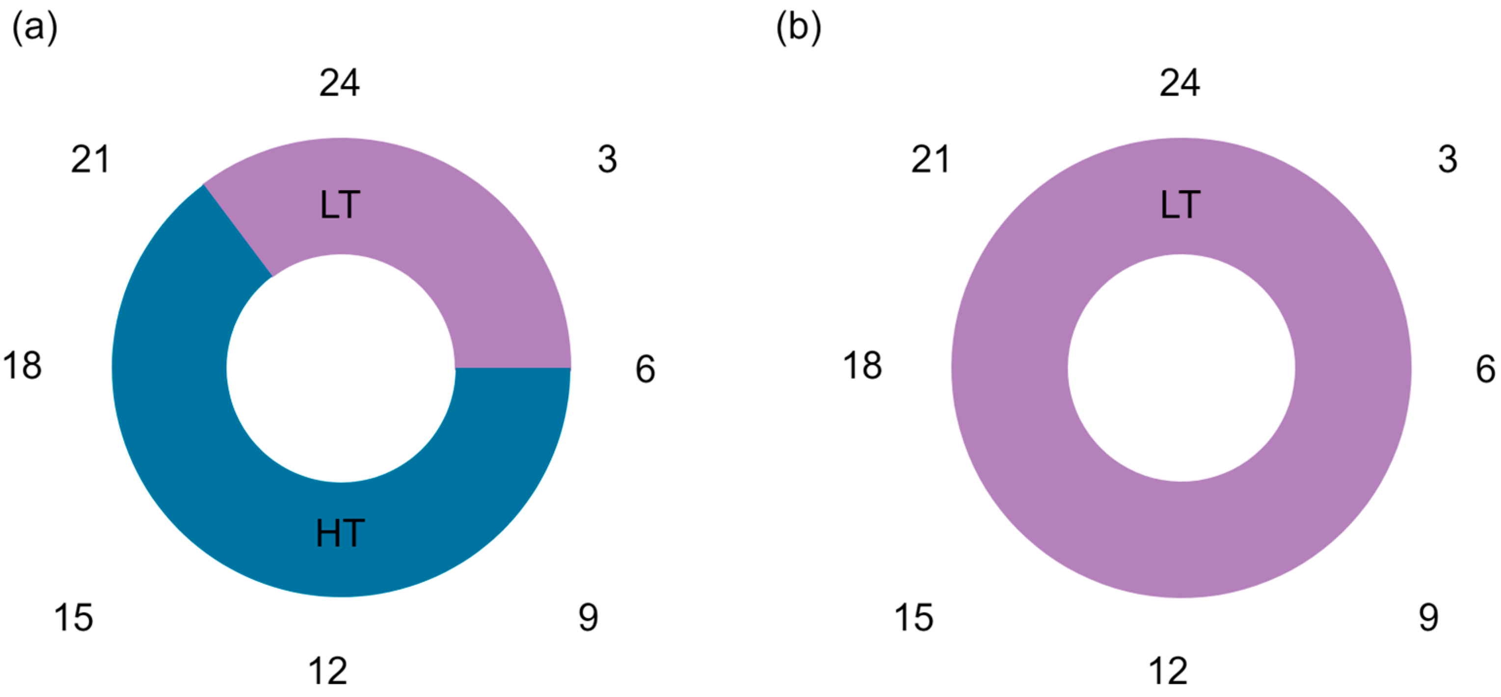
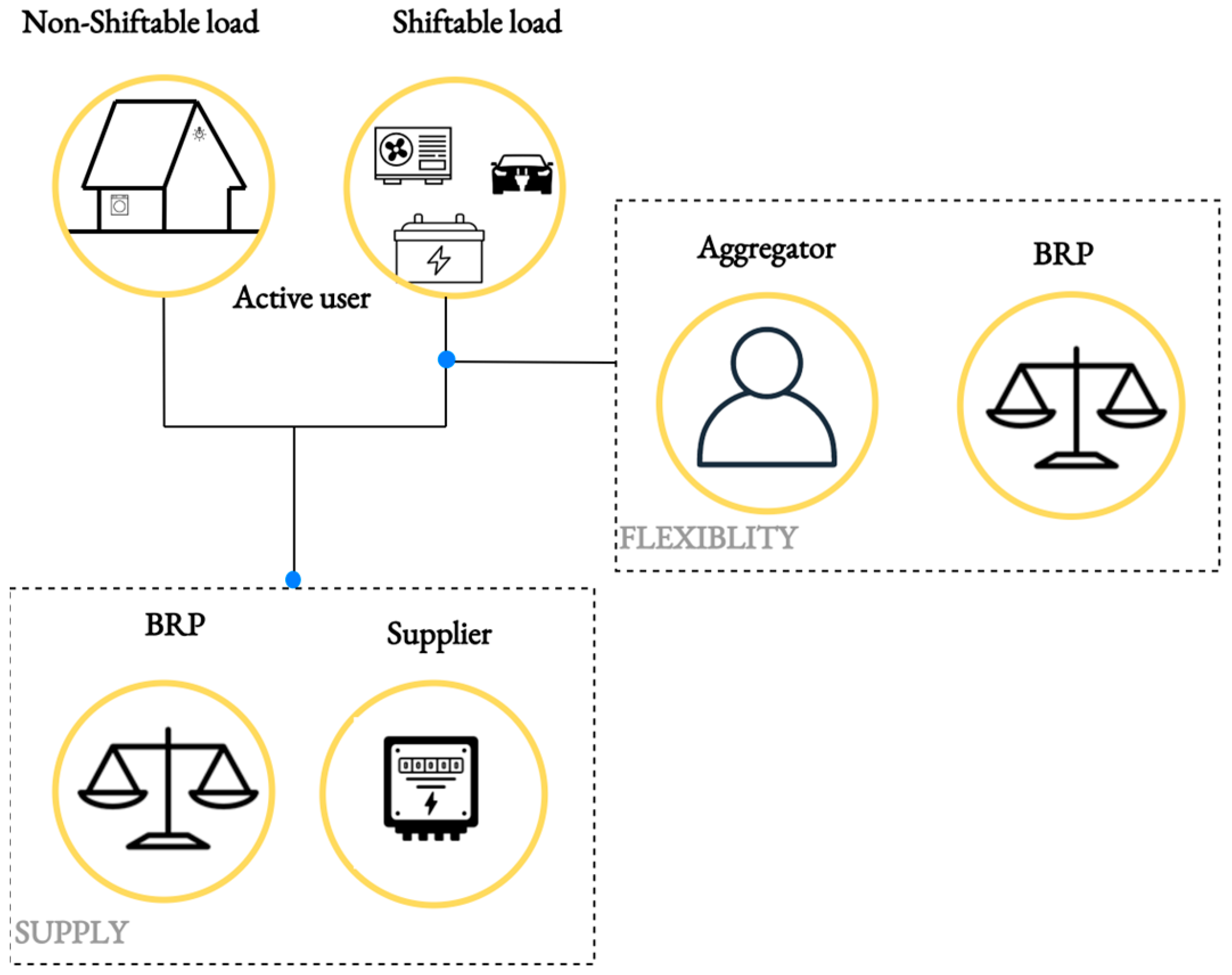
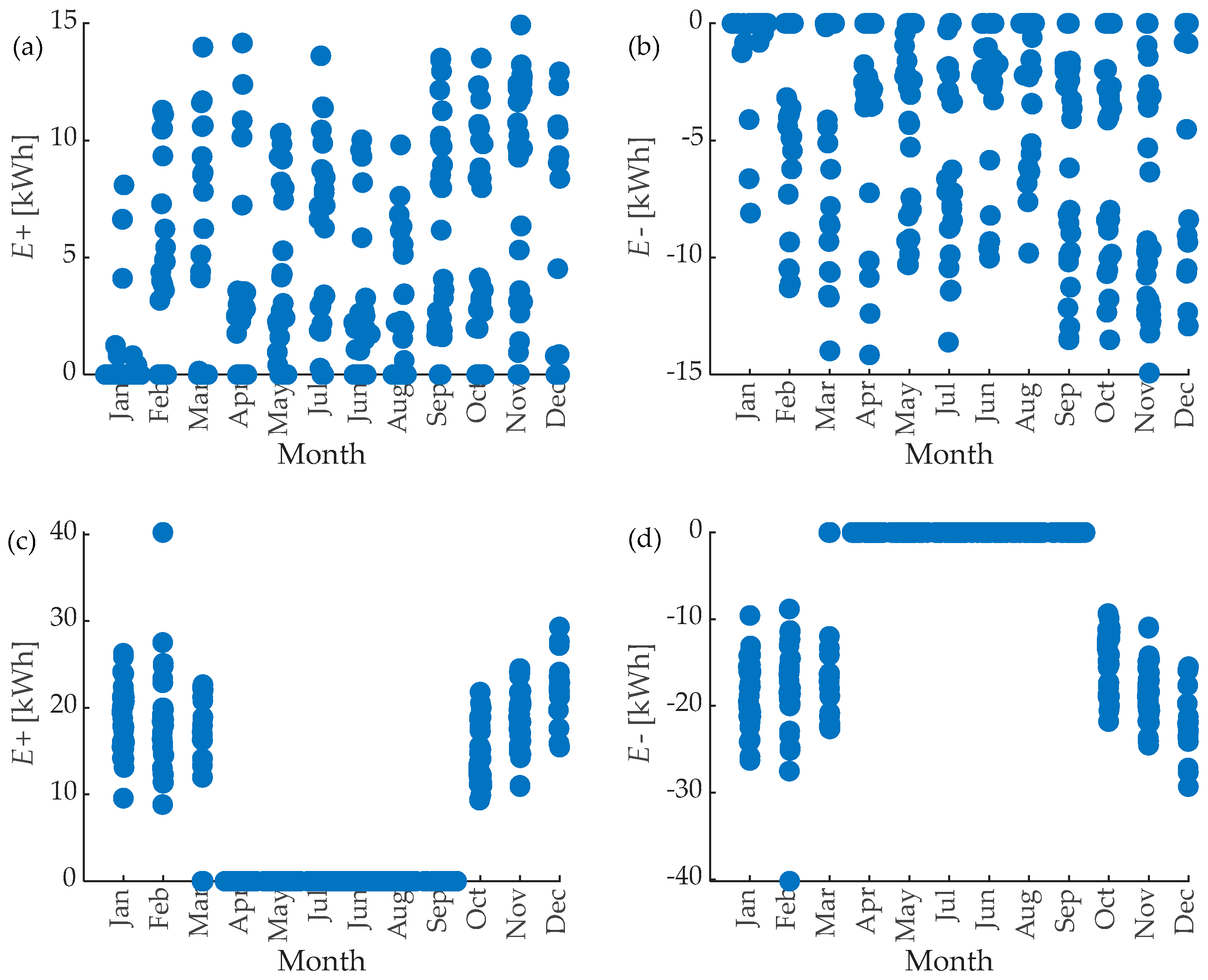
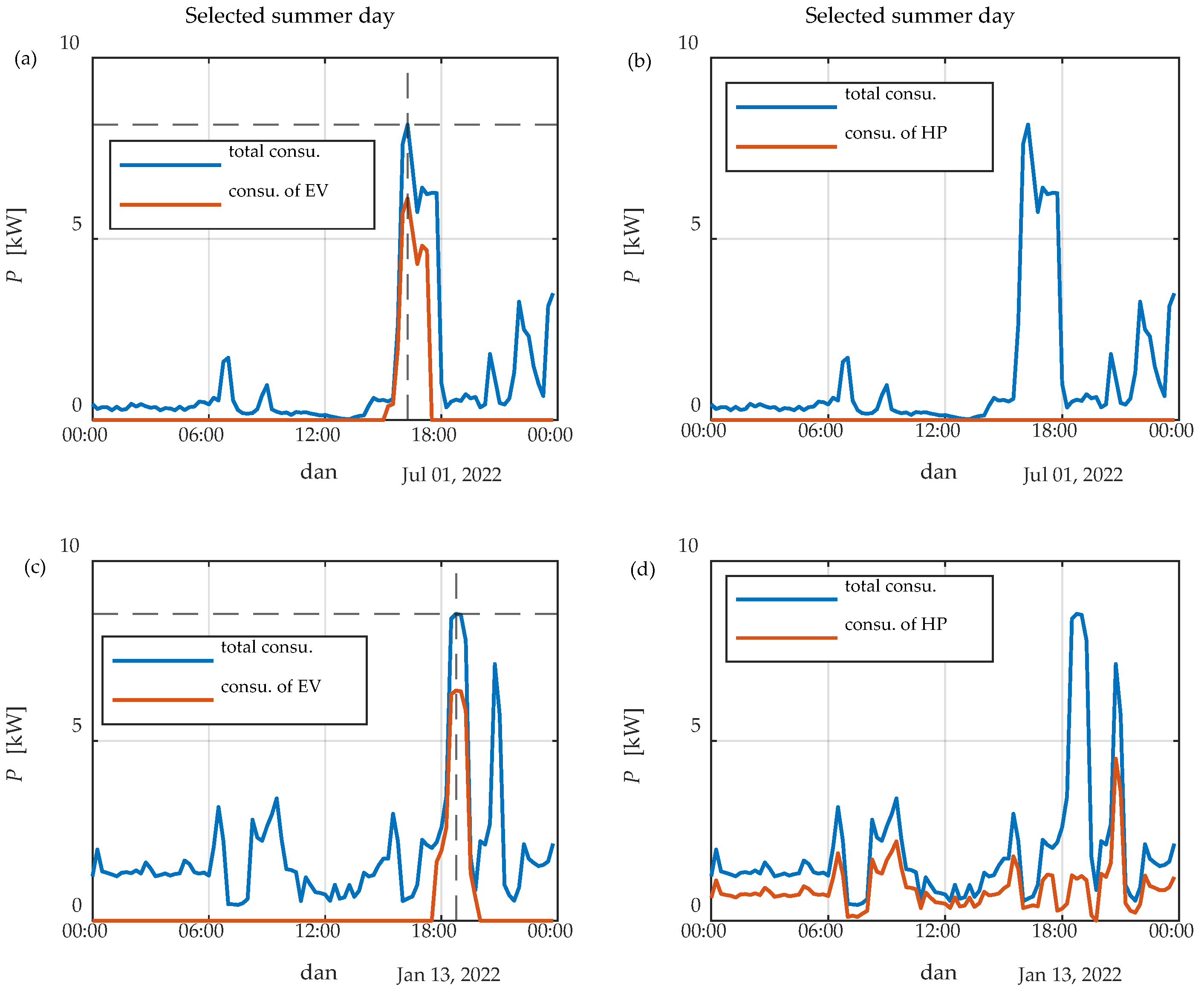
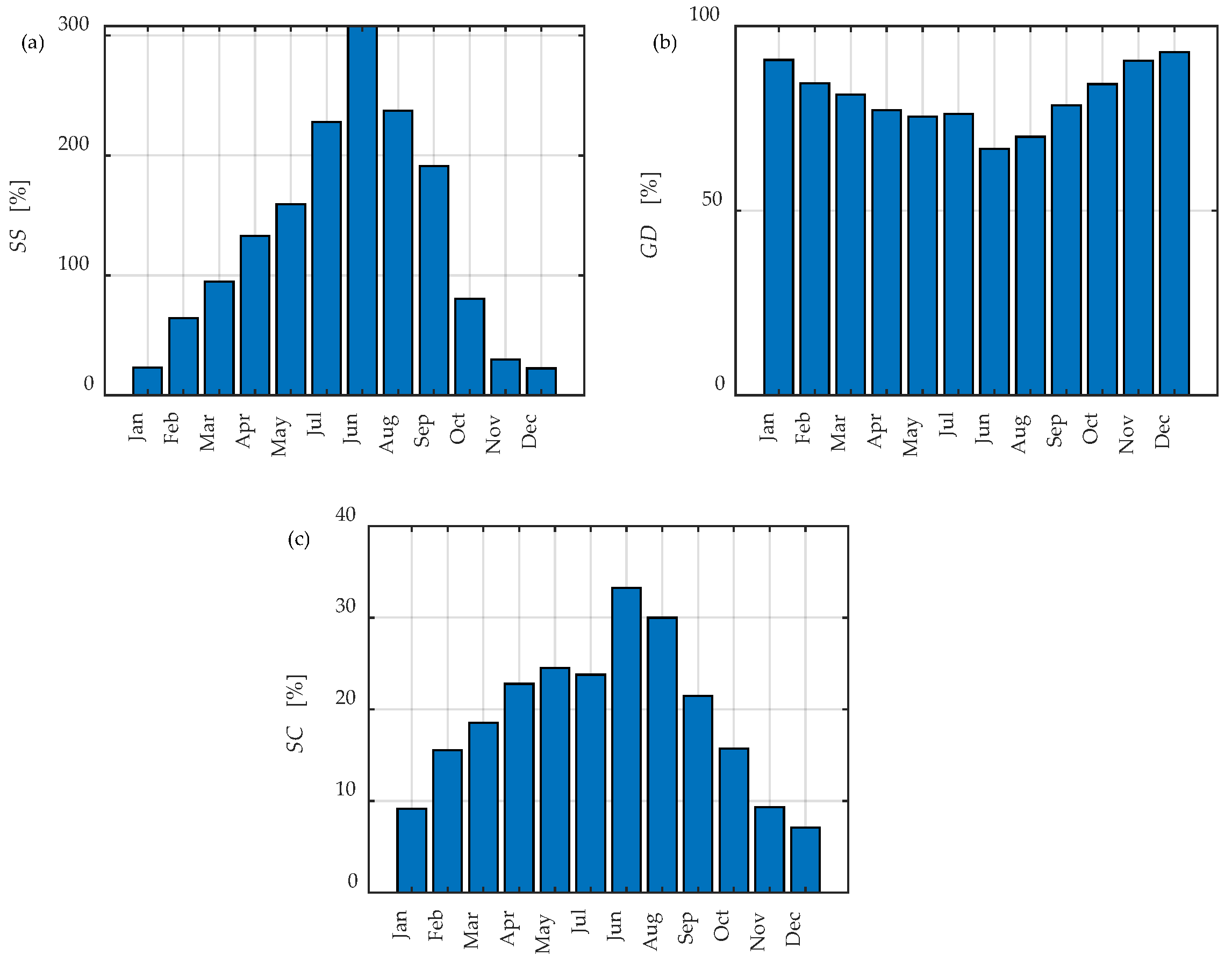
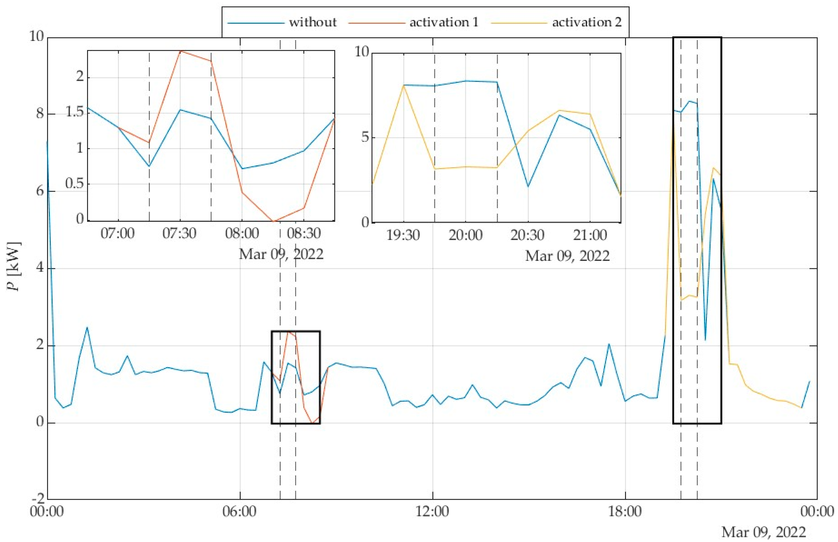
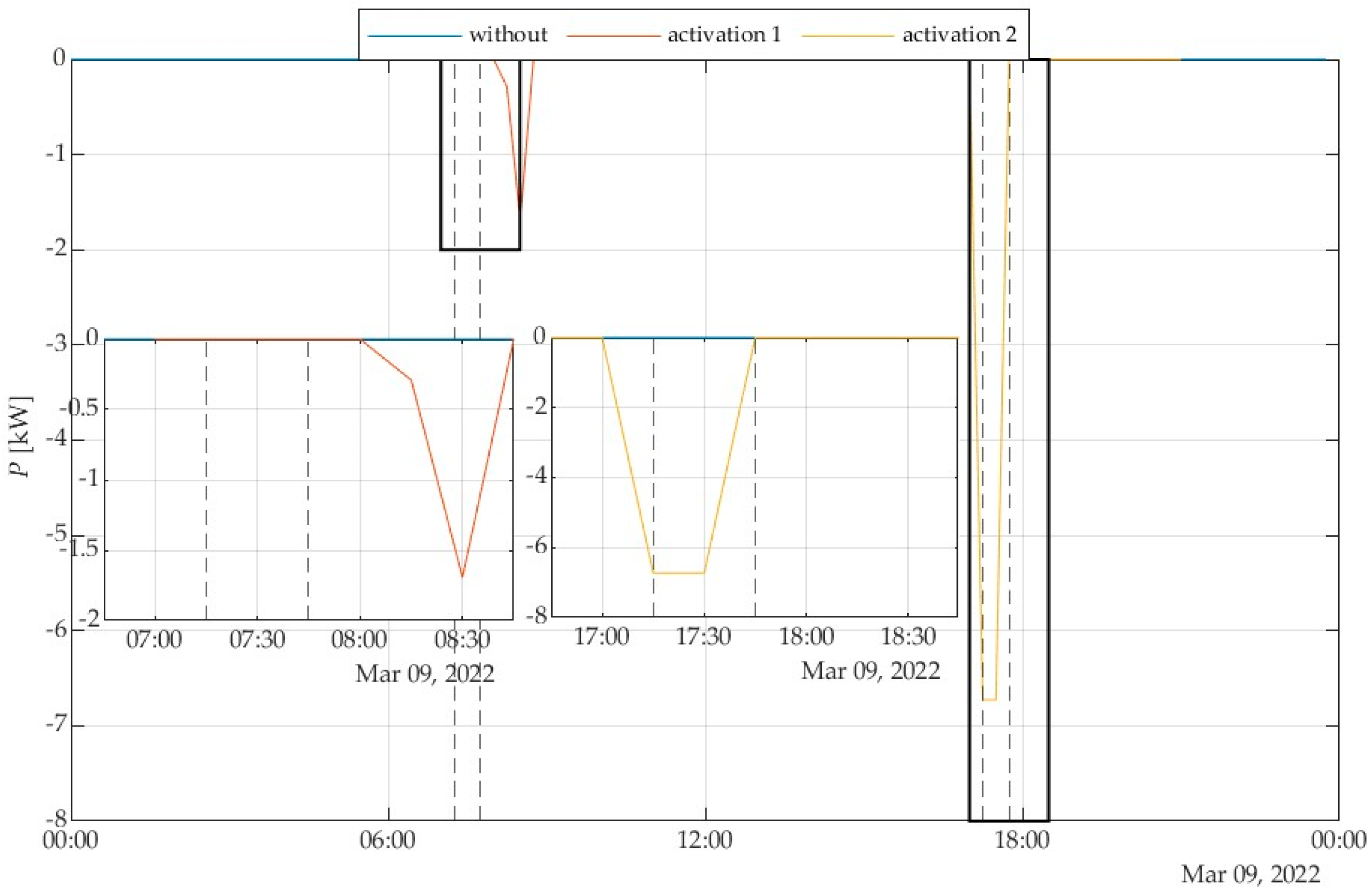
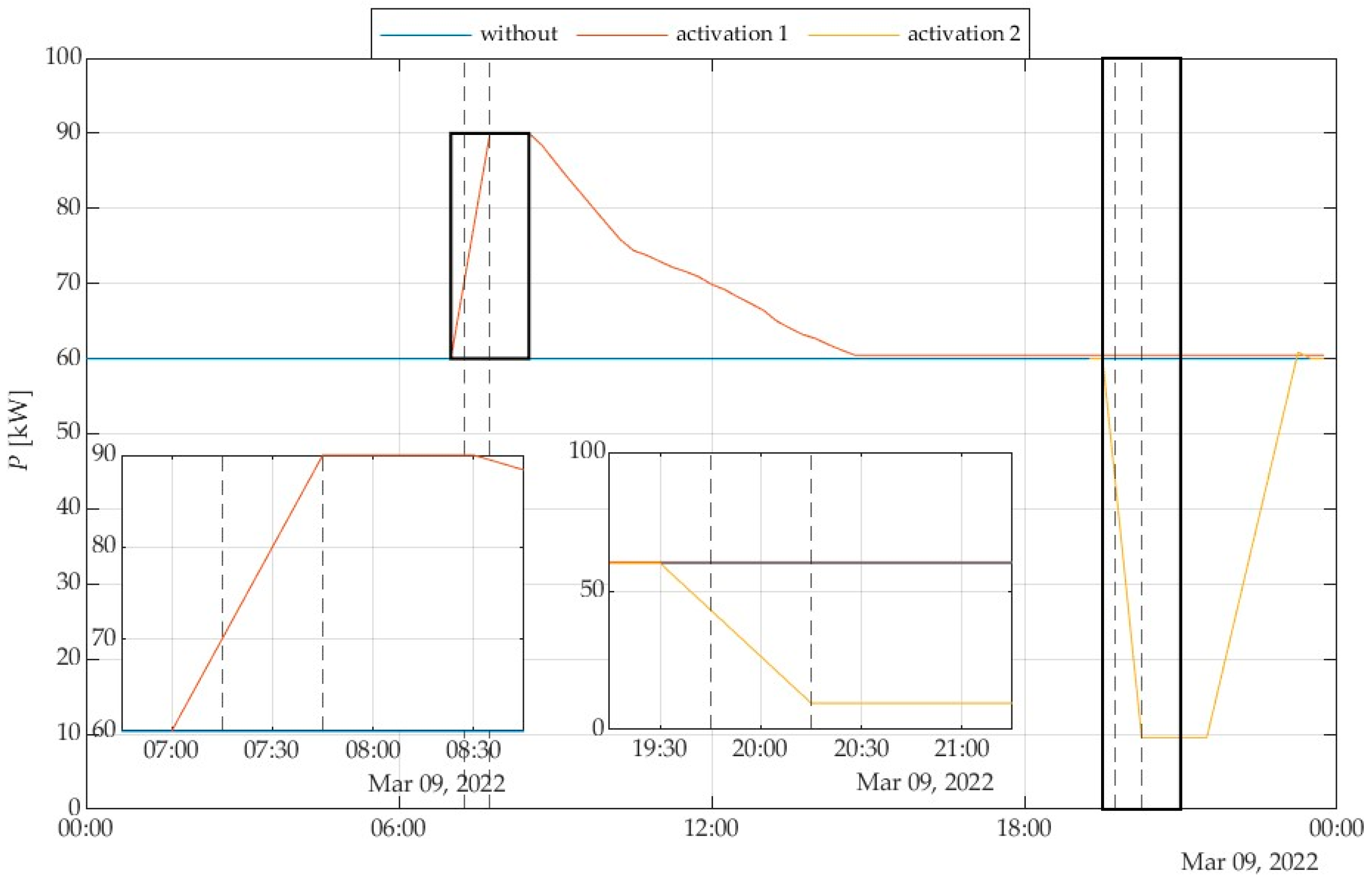
Table 1.
Charges and prices that are used to calculate the final price of electric energy for Slovenian households.
Table 1.
Charges and prices that are used to calculate the final price of electric energy for Slovenian households.
| PLT [EUR/kWh] | PHT [EUR/kWh] | NCLT [EUR/kWh] | NCHT [EUR/kWh] | CC [EUR/kW] | C1 [EUR/kWh] | C2 [EUR/kWh] | C3 [EUR/kW] | C4 [EUR/kWh] |
|---|---|---|---|---|---|---|---|---|
| 0.118 | 0.082 | 0.03215 | 0.04182 | 0.77417 | 0.00013 | 0.0008 | 0.36948 | 0.00153 |
Table 2.
Results of analysis without net metering.
| Strategy | Pd [EUR] | CBESS [kWh] | SS [%] | SC [%] | GD [%] |
|---|---|---|---|---|---|
| Without | 1401.2 | - | 107 | 17 | 83 |
| Without | 1116.0 | 10 | 107 | 36 | 64 |
Table 3.
Results from strategy 1 analysis.
| Strategy | CBESS [kWh] | fA | PPV_e [EUR] | Pd [EUR] |
|---|---|---|---|---|
| 1 | - | 0.2 | 599.7 | 801.5 |
| 1 | - | 0.4 | 1199.5 | 201.7 |
| 1 | - | 0.6 | 1.799.2 | −397.9 |
| 1 | 10 | 0.2 | 459.8 | 656.1 |
| 1 | 10 | 0.4 | 919.7 | 196.3 |
| 1 | 10 | 0.6 | 1379.5 | −263.54 |
Table 4.
Results for strategy 2.
| Strategy | CBESS [kWh] | fA | PPV_e [EUR] | Pd [EUR] | [kWh] | SS [%] | SC [%] | GD [%] |
|---|---|---|---|---|---|---|---|---|
| 2 | - | 1 | 26.6 | 1346.0 | 8.29 | 107 | 15 | 85 |
| 2 | 10 | 1 | 148.8 | 967.2 | 6.01 | 107 | 32 | 68 |
Disclaimer/Publisher’s Note: The statements, opinions and data contained in all publications are solely those of the individual author(s) and contributor(s) and not of MDPI and/or the editor(s). MDPI and/or the editor(s) disclaim responsibility for any injury to people or property resulting from any ideas, methods, instructions or products referred to in the content. |
© 2024 by the authors. Licensee MDPI, Basel, Switzerland. This article is an open access article distributed under the terms and conditions of the Creative Commons Attribution (CC BY) license (https://creativecommons.org/licenses/by/4.0/).
Share and Cite
MDPI and ACS Style
Tratnik, E.; Beković, M. Empowering Active Users: A Case Study with Economic Analysis of the Electric Energy Cost Calculation Post-Net-Metering Abolition in Slovenia. Energies 2024, 17, 1501. https://doi.org/10.3390/en17061501
AMA Style
Tratnik E, Beković M. Empowering Active Users: A Case Study with Economic Analysis of the Electric Energy Cost Calculation Post-Net-Metering Abolition in Slovenia. Energies. 2024; 17(6):1501. https://doi.org/10.3390/en17061501
Chicago/Turabian StyleTratnik, Eva, and Miloš Beković. 2024. "Empowering Active Users: A Case Study with Economic Analysis of the Electric Energy Cost Calculation Post-Net-Metering Abolition in Slovenia" Energies 17, no. 6: 1501. https://doi.org/10.3390/en17061501
Note that from the first issue of 2016, this journal uses article numbers instead of page numbers. See further details here.