


Operational Analysis of an Axial and Solid Double-Pole Configuration in a Permanent Magnet Flux-Switching Generator


1
Department of Electrical and Computer Engineering (DEEC), Instituto Superior Técnico, University of Lisbon, 1049 Lisbon, Portugal
2
Mechanical Engineering Institute (IDMEC), Instituto Superior Técnico, University of Lisbon, 1049 Lisbon, Portugal
*
Author to whom correspondence should be addressed.
Energies 2024, 17(7), 1698; https://doi.org/10.3390/en17071698
Submission received: 28 February 2024
/
Revised: 28 March 2024
/
Accepted: 29 March 2024
/
Published: 2 April 2024
(This article belongs to the Topic New Technological Solutions, Research Methods, Simulation and Analytical Models That Support the Development of Modern Transport Systems)
Abstract
:There are two main beneficial characteristics that doubly salient permanent magnet (PM) electrical machines present for aircraft applications: armature windings and PMs excitation sources placed on the stator side (maintenance and thermal management), and having a clear-cut rotor without PMs or excitation windings (vulnerable at high speeds due to associated centripetal mechanical stresses). Within this framework, a doubly salient permanent magnet (DSPM) generator was conceived by optimizing the stator size and rotor structure to minimize the torque ripple and maximize the root-mean-square (RMS) voltage value per turn of each generator phase. Firstly, a comparison between the 2D and 3D finite element method (FEM) models is made considering the results of 3D finite element analysis (FEA) as our benchmark in order to understand the accuracy of the 2D results against our benchmark model, the 3D one. A multi-objective design strategy based on a 2D FEA is made, it is set to have characteristics closest to optimal for a Boeing 767 turbine, that is, the necessary electromotive force for a required power of 90 kW at 3000 rpm, feeding a simplified Boeing 767 electrical power distribution system. The results show that the machine could not deliver the required power at 3000 rpm since the 2D FEA demonstrates that the 2D model gives optimistic results when compared with the 3D FEM model. However, with a 3D FEA of the machine feeding the aircraft load, it was seen that the machine’s efficiency is 92%, suggesting that this machine can be a plausible solution.
1. Introduction
Some generators of aircraft power generation systems are synchronous machines with permanent magnets (PMs) [1,2]. A higher power density and efficiency and being more compact and lighter due to the lack of any slip-ring-based external excitation are some advantages [3]. However, one emerging machine topology is the flux-switching machine, or, more specifically, doubly salient machine, due to its higher reliability at higher rotor speeds due to its simple rotor design [4]. This mechanical characteristic is the main reason for studying a DSPM topology generator suitable for integration into aircraft fuselage since it must endure all atmospheric conditions with the utmost reliability. The electromechanical torque will be our study benchmark for the optimization process to obtain the highest possible output power of the generator, optimizing only the 2D geometry of the generator. Nevertheless, other points of the study are the reduction in the vibrations and electromagnetic forces transmitted to PMs due to being placed in a stator iron core [5] and the reduction in the temperature decaying flux effect in PMs due to the better temperature dissipation [6].
Still, the current aircraft electrical generation systems can be separated into two kinds of technology: variable-speed constant-frequency systems and constant-speed constant-frequency systems [1,7]. The integrated drive generator (IDG) is commonly denominated as a constant-speed constant-frequency system. Most of the civil aircraft use this technology [7], which comprises a continuously set variable-speed (CVT) gearbox and generator. The integration of a CVT becomes a useful resource in this area since it gives the possibility to offer solutions with constant-frequency AC generation systems [8]. A lower reliability and efficiency and higher weight are the main drawbacks of [1,8]. The growing demand for the electrification of aircraft motivates the development of new solutions. A new trend in research involves exploring the potential of integrating generators within the structure of aircraft turbines, particularly for high-range aircraft, known as aircraft embedded generation systems. In the work of [2], it was verified that, inside the low-pressure turbine casing, there exists an enclosed space capable of accommodating a generator without compromising the aerodynamics of the turbine. Some advantages over the IDG can be depicted: being lighter, more efficient and reliable, less costly, and having easier integration on aircraft fuselage systems. However, the increase in the complexity of designing the turbines can be one drawback.
Consequently, the research aim is to integrate the DSPM generator into the aircraft fuselage, assuming an IDG solution since it is a mature technology. Nevertheless, the possibility of integrating the generator inside the aircraft turbine as an embedded generation solution is investigated.
2. Doubly Salient Permanent Magnet (DSPM) Machine and Methodology of Study Overview
The starting point of this project is the DSPM obtained in [9], which is presented in Figure 1. This machine is now going to be called the DSPM S4R5. Also, the methodology used to study the different DSPM geometries will be reviewed. The finite element analysis (FEA) will be our benchmark study of this machine using a distributed-parameter simulation environment finite element method (FEM) program. More specifically, for all multiphysics 2D and 3D FEM simulations, the software used was Comsol Multiphysics version 6.1. So, it will be depicted to understand how the FEM models are built. Finally, an overview of the optimization process is presented.
2.1. Geometry
Figure 1 shows the parameters relative to the 2D plot of the DSPM S4R5 geometry. Table 1 presents the machine dimensions of Figure 1. corresponds to the active length of the machine or stack iron length. The 3D plot is shown in the next section.
The main geometric feature of the machine is the shape of the rotor teeth, which is given by a quadratic Bézier curve. In a Bézier curve, the initial and final points belong to it, while the intermediate control points (for a quadratic curve, there is only one intermediate control point) determine the curvature of the curve [10]. The minimum airgap value considered is 1.6 mm as a minimum mechanical safety margin. The coils have 20 turns each for the initial geometry’s number of turns (). Nevertheless, during the geometry optimization process, one turn is assumed for the sake of simplicity.
2.2. Materials
The materials corresponding to the different components of the machine are presented in Figure 2. The PMs are highlighted in Figure 2 by zooming in on one of them.
For the iron core, Silicon Steel NGO 35JN200, which has a 0.35 mm lamination thickness, is considered. Its density () is 7600 kg/m3, with a B-H characteristic curve presented in Figure 3 as assumed in [9] and its electrical conductivity () of 1 S/m being considered as isotropic conductivity to reduce computational time.
The NdFeB magnets present a B-H curve given by a slope with a remanent flux density () of 1.4 T with a coercive magnetic field of 1.08 MA/m. Their relative magnetic permeability () is around 1.03. The electrical conductivity of the PM is assumed to have a value of 1 S/m to mitigate simulation errors of induced currents. Also, the density of the PMs () is 7600 kg/m3.
The copper windings are considered to have a relative magnetic permeability and relative electrical permittivity similar to the air. However, their electrical conductivity () has a value of 60 MS/m. Figure 4 shows the coil numbering and the permanent magnet orientation.
2.3. Generator Specifications
The pretended specifications for this aircraft are based on [9,11]. So, the needed electrical apparent power output is at least 90 kVA at a speed of 3000 rpm. As detailed later, values such as phase voltage and current will depend on the final design achieved and the AC/DC/AC power converters feeding the electric load typical of a 767 aircraft.
The aircraft load is simulated as a load fed by an AC/DC/AC converter. Therefore, for simplification, the rectifier (AC/DC converter) is considered to have properly dimensioned LC filters to have a two-level square current wave as phase current during the optimization process.
The assumed value of nominal current density for the coils is 5 [A/mm2], with a filling factor of 0.5 to ensure the thermal limits and a normal slot factor [12].
2.4. FEM Study of DSPM S4R5 Machine
The equations that govern the FEM models are presented in Equations (1) and (2), where is the magnetic field vector, is the magnetic flux density vector, and is the current density vector.
The magnetic vector potential equations are considered for the stator side since currents are applied to the coils, and the magnetic scalar potential equations are neglected on the rotor side since the eddy currents in the rotor are neglected.
2.4.1. Magnetic Flux and Torque Calculation
The study of magnetic flux () and torque (T) is relevant since these components relate to the output power, input power, and mechanical vibrations, respectively. Therefore, the study process of these quantities considers an angular variation in the rotor position of , which corresponds to an electrical cycle.
Magnetic Flux Calculation
For the 3D model, an FEA is performed assuming a stationary condition, while, for 2D geometries, the FEA considers a time-dependent study since our work verified that the time-dependent study is faster than a stationary one in this condition.
The induced voltage calculation in a stationary situation for 3D geometries is obtained by running the gradient of flux to the position of the rotor since the rotor speed is assumed to be constant. This avoids a time-consuming, time-dependent study.
Electromagnetic Torque Calculation: Arkkio’s Method
The software Comsol 6.1 can perform torque computation through Maxwell’s stress tensor or by Arkkio’s method [13], characterized by a better precision than normal Maxwell’s stress tensor. Like magnetic flux computation, the study of torque (T) will be time-dependent for 2D geometry and stationary for 3D geometry, remembering that the rotor rotates an electrical cycle.
2.4.2. Iron Losses Determination
Modeling of Iron Losses
The iron losses model assumed builds on Bertotti’s model, where Equation (3) presents the equation that governs the model. The variables , f, , , , and are the iron losses [W], the frequency [Hz], the peak value of the signal of the magnetic flux density [T], and the dimensionless coefficients of hysteresis, eddy current, and excess losses, respectively.
Iron Losses’ Data Map
The majority of power loss data of the Silicon Steel 35JN200 is extracted from the power loss manufacturer’s table. However, the remaining missing data are obtained by extrapolating the manufacturer’s data by fitting those data with the iron losses model Equation (3). The Berttoti coefficients are obtained by the data fitting for different frequencies. Figure 5 shows 3D graphs to better visualize the values of losses in iron with the level of induction, as well as the frequency relative to the extrapolation of the range of the most significant harmonic components of the magnetic flux density evolution.
Determination of Iron Losses
As a first step, acquiring in the entire mesh and assuming two electrical cycles is necessary for accurate fast Fourier transform (FFT) computation. With those harmonic values of magnetic flux density, it is possible to obtain the massic losses in the machine’s core by interpolating those values with the power loss data shown in Figure 5. Moreover, the data obtained from FEM software also provide two other matrices: the identification of the element nodes and their geometric coordinates. This allows us to compute the volume of each element for either 2D geometries or 3D geometries. After obtaining the total volume of each element, knowing the value of massic losses in each element and its density, the total value of iron losses is given by Equation (4), where k is relative to the mesh elements. , , , are the iron losses in the core [W], the massic iron losses in each mesh element [W/kg], the volume of each element [m3], and the density of the material that corresponds the element [kg/m3], respectively.
2.4.3. Electrical Equivalent Circuit Study
The equivalent electric circuit is based on a first-order state-space model as shown in Equation (5), where the state variable is the phase current. The matrices , , , , and are the resistance matrix, inductance matrix, matrix, voltage vector, and current vector, respectively. Those first three matrices are represented in Equation (6). For the sake of simplicity, the phase current is considered the output variable, and the rotor speed () and voltage are considered the input variables. This analysis considers one phase per pole, so a four-phase system.
Firstly, we start to determine the parameters of the equivalent circuit model using the FEM model. The FEM simulation software determines the resistive value of the windings () by the quotient of the product between the number of turns in the winding () and the average length of the coil () by the product between and the cross-section area of the wire of the winding (). Recalling the axial symmetry in 3D geometry, the resistive value in 3D is multiplied by two.
Using FEA results, the inductance and N maps are obtained by the gradient of each phase’s linked flux to the current and rotor position, respectively. However, taking into account that the study is based on only the phase current of coil 1, the inductance maps obtained will reflect one phase, phase 1, which corresponds to the first column of . The column vector is given by the derivative of the linked flux of the coils to the rotor position. Equation (7) shows and matrices.
Afterward, since there is symmetry between electrical cycles, only one electric cycle was simulated using a stationary study. Visual observation of the linked flux evolution of phase 1 indicates that the maximum and minimum values of linked flux correspond to the location of the d and q axes, respectively. To corroborate the location of the dq axis, one sets out the value of Br to 1.4 T and makes the stationary study once again to obtain torque evolution since the electromagnetic torque is higher when the rotor is aligned with the d-axis than when it is aligned with the q-axis.
2.5. Geometry Optimization
2.5.1. Optimization Objectives
The objective functions considered are the minimization of useless torque () and the maximization of torque density (). Since our study focuses on maximizing the output electric power and is made at stationary conditions, the average value of input electromechanical torque is a good gauge for maximization. However, without belittling, minimizing the vibrations transmitted to the PMs is also considered to diminish the oscillatory component of the electromechanical torque. These objectives are shown in Equation (8).
2.5.2. Design Variables
This thesis will study the effect of geometric dimensions in electromechanical torque. So, to maximize the freedom degree of the optimization, it will consider almost all geometric independent variables as decision variables as exposed in Figure 1, which are , , , , , g, , , , , , , , , and .
2.5.3. Constraints
According to Figure 1, it is possible to observe that there are geometrical constraints that cannot be violated so that there are no intersections between the different DSPM machine elements. Therefore, the geometrical constraints are enumerated below.
The limits of the design variables are presented in Table 2.
2.5.4. Optimization Program: Genetic Algorithm
To perform the optimization, the NSGA-II (Non-Sorting Dominant Genetic Algorithm) algorithm is used, which is based on the basic idea of the evolution of populations throughout generations, considering a sufficient number of generations to acquire the Pareto front or curve [14], where, next, the optimization algorithm is briefly described.
Considering the operation principle of the NSGA-II algorithm, the optimization process starts evaluating the constraints violated to study only the valid geometries. The admissible geometries are studied in a stationary study of an electrical cycle, and its results are sorted as described previously to make the next generation. This process is repeated to the next generations until the Pareto curve converges. The number of generations and the number of individuals considered are at least 150 [15] and 75, respectively. Figure 6 illustrates a flowchart of the whole process considering the NSGA-II algorithm and electromagnetic study algorithm to visualize the parallelism of the processes in the optimization.
3. Results
3.1. Comparison of Flux and Torque Calculations Based on 2D and 3D Geometries at No Load and Lumped Parameters Study
Figure 7 illustrates, on the left side, the DSPM S4R5 and, on the right side, the axial symmetry of the DSPM S4R5 model used to reduce computational time. The PMs are represented in blue to highlight their visualization. Also, Figure 8 shows the corresponding 2D geometry.
Figure 9 shows that the 3D geometry has a higher average and lower peak-to-peak amplitude values of linked flux than its 2D counterpart. As 3D geometry presents lower magnetic reluctance from the standpoints of the PMs, this means a rise in their magnetic load and, in turn, in their total magnetic flux. The constraints imposed on leakage paths by the 2D geometry compel the magnetic flux to cross from the stator into the rotor. In short, as 2D geometry gives more optimistic results in output voltage than 3D geometry, 2D geometry can only be used in the preliminary phase of designing machines with large diameter–length ratios.
The linked flux evolution, as an image of the induced voltage, is studied to analyze the voltage quality. So, the computation of the weighted total harmonic distortion (WTHD) of linked flux is performed as shown in Figure 9. The WTHD is given by Equation (9) [17].
The WTHD for 2D geometry is approximately 4.17%, and the WTHD for the 3D one is approximately 4.25%, thus demonstrating that the 2D geometry has a good approximation to the 3D geometry in no-load conditions. This means that the voltage quality can be analyzed using 2D geometry to reduce computational time.
On the other hand, as described in Section 2.4.1, Figure 10 is obtained regarding the electromechanical torque evolution.
The 3D results present a certain unexpected ripple in torque. The torque data were not processed to maintain the peaks since our study verified that smoothing the data imposes a deviation in peaks. The ripple effect is caused by the inaccuracy of the mesh and stationary study. As in 2D geometry, the torque amplitude is higher, which means that 2D geometry gives more conservative results on oscillatory torque than its 3D counterpart. So, once more, 2D must be used only in a preliminary design phase. To obtain more accurate results, 3D geometry must be used.
As the study of magnetic flux was already made, a study of the lumped-element parameters of the equivalent electric model of the machine is performed, as described in Section 2.4.1. The stator coil resistance is 7.2 . We recall that the windings have only 20 turns to a total active cross-section of 543 mm2, meaning a value of 27.15 mm2 of the cross-section of each turn.
Figure 11 and Figure 12 show the preponderance of the effects of the rotor position in inductance fluctuation compared to the effects of phase current. The peak-to-peak value of 300 due to the rotor position effect and a neglectable peak-to-peak value due to the phase current effect justify the previous sentence. Therefore, the core saturation effect is not visible. The self-inductance is about five times greater than the adjacent mutual inductances and around seven times higher than the opposite mutual inductance. Their geometrical arrangement gives the differences between mutual inductance values, either mean or oscillatory values. Relative to the parameter N, these maps relate the EMF produced by the DSPM S4R5 machine with the rotor position and the current apart from rotor speed as displayed in Equation (5). Moreover, it is highlighted that the decaying effect due to the current is similar for the N maps to the linked flux maps.
3.2. Iron Loss Calculations at No Load
The method discussed in Section 2.4.2 applied to 3D geometries will be our benchmark since the 3D geometry is the most accurate model. Therefore, the loss values obtained for 2D and 3D geometry are 362W and 284W, respectively.
Thus, the 2D geometry results present an oversize of about 45% concerning the most accurate value, 3D geometry. Once more, this means that the 2D model enables a rough estimation of iron losses in the preliminary phase of the design of machines with a large diameter–length ratio. Due to the high discrepancy in results, the 3D geometry must be used for improved accuracy.
3.3. Phase Current Shape Study
This study is based on the results of [18,19,20], where four current waveforms are seen as a sinusoidal waveform, a square waveform, and two rectified sinusoidal waveforms.
The different kinds of waveforms of current assumed to be studied are shown in Figure 13 for only one phase current with an amplitude of 110 A. Also, it is highlighted that the number of points considered to acquire the results is enough to represent the fast transitions of the waveforms with the required accuracy. For the sinusoidal waveform, the power angle that provides the biggest torque mean value is 0°.
Most current waveforms in Figure 13 derive from a cosine wave, where the blue one is the proper one. To replicate a current waveform given by a power electronic converter, the waves in the orange and violet lines are the cosine waves considering firing angles. However, as the theory of conventional switched reluctance machines mentions, the higher output power is given when the range given by firing angles is in the interval where the inductance of the machine is decreasing. So, a square wave is obtained (green color).
Table 3 shows the average reaction torque value results, the standard deviation of the torque to represent the oscillatory torque, and the ratio between them.
The best waveform is the square waveform, which occurs when imposed at the moment, and a misalignment of the rotor and stator poles occurs since it has the lowest ratio. So, the square current waveform will be used in the optimization process. Also, the phase current waveform can significantly improve the electromechanical torque mean value and, in turn, the delivery of active power.
3.4. Optimization of the DSPM S4R5 Machine Results
The best front obtained by the optimization process is illustrated in the left part of Figure 14. The selected point is in the middle part of the Pareto curve. The region above the red line represents an output power equal to the minimal power requirements of 90 kW, considering 3000 rpm. The right part of Figure 14 illustrates the geometry representative of the selected point.
The geometry obtained has a decrease in its total volume, concerning the initial geometry, of around 35%, by a reduction in its radius to about 19.4% relative to the initial geometry. The most relevant difference is the rotor teeth design, approximating a rectangular shape like the classical switched reluctance machines’ rotors. The main geometrical parameters of the machine are exposed in Table 4.
Moreover, to visualize the behavior of this new optimal geometry with nominal load, Figure 15 and Figure 16 illustrate the magnetic flux and torque evolution along an electrical cycle for the 3D geometry.
The torque presents a sharp evolution when the stator poles are almost at the right and when right after the alignment, which can impose mechanical stress on the material. However, as the peaks are at around 10% of the nominal mean value of the electromechanical torque, the mechanical stress is not harsh. The linked flux evolution presents discontinuity zones due to the imposed switching load currents, translating into voltage peaks.
Figure 17 and Figure 18 show the results for the 3D geometry of torque and linked flux in the same load condition as the 2D geometry. Once more, these results are our benchmark results.
The mean value of linked flux and electromechanical torque decreased. The average value of torque has a decrease of around 46.5%, meaning that the selection of the geometries of the optimization process must take that into account. The average of the electromechanical power is about 47.75 kW. Also, the average value of linked flux decreased its value by 82.8%, and the maximum value decreased by about 45%, indicating that the 2D geometry gives errors above 10% compared to 3D geometry for the linked flux values of large-diameter–length ratio machines in load conditions. In short, this confirms that the 2D model must be oversized for high-diameter–length ratio machines to attain the requirements in the most accurate 3D model.
The voltages, currents, and total electric instantaneous power are presented in Figure 19, Figure 20 and Figure 21. The indexes 1, 2, 3, and 4 shown in the legends are relative to coils 1, 2, 3, and 4. It is recalled that the voltages were obtained without considering the resistive voltage drops of coils since, for one turn, these components were around three orders of magnitude below the output voltage value. Nevertheless, we recall that the generator voltage distortion does not affect the load since it is considered an electronic interface with respective AC filters between the generator and load that must guarantee that the load voltage has low WTHD.
As visualized in Figure 18, the voltages are highly distorted as linked flux due to the imposition of pulsed currents. The transient zones of the commutation of the current cause voltage peaks. So, the peaks seen in the power are derived from that fact.
The difference between the average output power and average input power could occur due to the lack of accuracy of the results. During the work of this dissertation, the torque results were more accurate than the voltage results. So, our benchmark is the electromechanical torque. This indicates that, for studying electrical power, it is necessary to use a simpler model: the electric equivalent model of the DSPM S4R5.
Although knowing that the Joule losses and iron losses can be studied, the efficiency of the machine is given by the quotient of the difference between the total mechanical power and the studied losses by the proper total mechanical power. As visualized in Figure 20 and Figure 21, the four phases are switched on by a quarter of the electrical period. So, relative to the Joule losses, this means that it can be computed for a single coil, presenting a value of 722 W. The iron losses computed as mentioned in Section 2.4.2 have a value of 3.05 kW. So, the efficiency of the optimized machine is around 92%, neglecting mechanical losses. This efficiency value is acceptable since the optimization process did not consider this aspect.
3.5. Comparison of Initial and Optimized Geometries at No Load and Lumped Parameters Study
The initial geometry is recalled to visualize its differences to the optimized geometry, being the first one illustrated in Figure 22 and the last in Figure 23.
To compare with [9], the number of turns per coil is now assumed to be 20. Figure 24 shows the evolution of the linked flux for the initial and optimized machines in order to compare both. The major difference remains in the mean value since the optimized geometry presents a reduction of 42.9% relative to the initial one. Besides that, it is observable that the peak-to-peak value of the optimized geometry is about 60 mWb compared to 50 mWb. This translates into a higher output voltage considering the same rotor speed for both geometries.
Once more, using the WTHD in linked flux waveform to compare the voltage waveform quality, the WTHD value is 1.1% compared to 4.2%. This means that the voltage quality of the optimized DSPM S4R5 machine is greater than the original one.
Figure 25 illustrates the electromagnetic torque for the initial and optimized 3D machines for comparison purposes. The evolution in the lower peaks is less rough in the new geometry than in the original one since there is just one abrupt variation in those peaks instead of two, as in the initial geometry. This helps to minimize the mechanical stress imposed on the shaft. Once more, the results present a significant ripple because they are not filtered since the smoothing would distort the peak values.
For the comparison of iron losses of the original and optimized DSPM S4R5 machines, the iron losses calculation was made by an element method as described in Section 2.4.2, obtaining 286 W for the original geometry and 204 W for the optimized geometry. Thus, it can be verified that there is a reduction of 28.67% in core losses compared with the original geometry. As the rotor speed of both machines is 3000 rpm, the difference between them, according to Equation (3), is the magnetic flux density in the core of both machines. Since the harmonic spectrum of linked flux reflects the behavior of each harmonic of magnetic flux density, the WTHD is a measure of the higher harmonics amplitude relative to the fundamental one. So, as the WTHD of the linked flux of the optimized geometry is lower than the original geometry, the decaying of the harmonic components for the optimized geometry is higher than the initial geometry. This means that the main difference between the machines is the lower harmonic component of the optimized one.
The lumped parameters representation of the optimized machine is studied, as referred to in Section 2.4.1 and Section 3.1. The stator coil resistance has an ohmic value of 0.62 .
Figure 26 and Figure 27 show each coil’s inductance and N maps. Once more, the inductance of the machine is higher in the aligned position than in the misaligned position. Figure 26 shows, for coil 1, its self-inductance and the mutual inductances with coils 2, 3, and 4. By making a comparison between Figure 11 and Figure 26, it can be observed that the self- and mutual inductances of the optimized machine have lower values than the original one. The superiority of self-inductance over mutual inductance is similar to what was seen in Section 3 since there is a proportionality that is around four times greater for the mutual inductance of adjacent phases and around five times greater for the inductance of the opposite phase. The N parameter tends to be a more sinusoidal wave than the initial geometry, as verified by the reduction in the value of WTHD, which implies a non-oversizing of the filters of the converter. The peak values are similar between the geometries. So, considering constant rotor speed, the induced voltage generated is expected to be the same for both geometries in no-load conditions. Once more, the yellow and blue colors represent each map’s higher and lower inductance values. In essence, the optimization process studied allows for improving the overall electric performance of the DSPM S4R5.
3.6. Loading Analysis of the Optimized Geometry
3.6.1. Aircraft Equivalent Electrical System
To study the optimized generator in an electric circuit, the equivalent circuit of the aircraft is considered, as depicted in [11]. The generator is modeled by a controlled current source, which is the control signal given by the equivalent electric system. The voltage measurement of each controlled current source gives the system feedback.
3.6.2. Electrical Response of the Generator with Non-Commanded AC/DC Converter
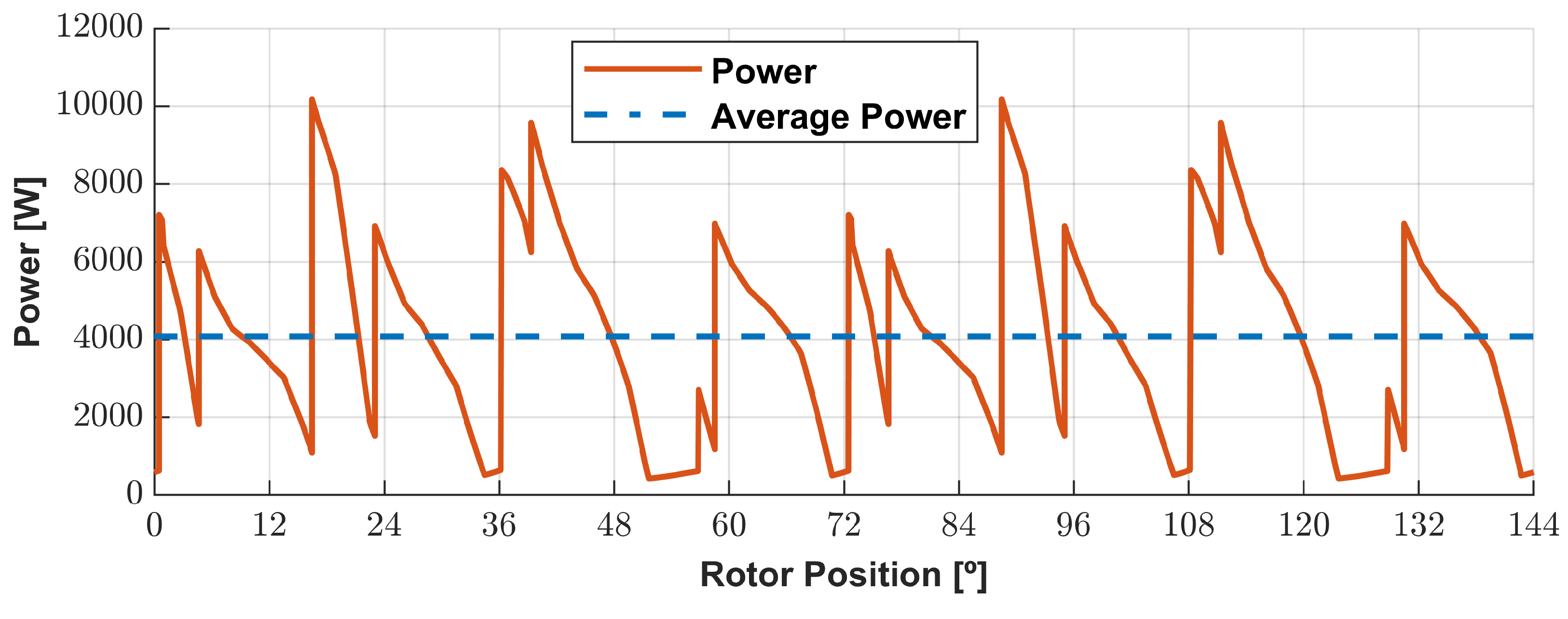
The simulation of the equivalent electric system of the aircraft studied in [11] and the equivalent model proceeded in a lumped-parameter circuit software using the methodology described in Section 2. Figure 28 and Figure 29 illustrate the evolution of the voltages and the currents of each coil. The voltage waveform of each coil is highly distorted due to the no-load situation since the AC and DC filters were not properly adjusted for this generator. Also, the voltage waveforms between coils are not symmetrical. Figure 30 represents the generator output’s instantaneous power evolution. The average output power is around 4 kW, well below the output power obtained in the ideal case. The voltage decaying is abrupt just after the peak, implying an abrupt output power decrease. So, the lack of control implies a degradation in the electric performance of the generator, which results in a significant reduction in its output power. This shows the need to design a control system to improve the DSPM performance.
4. Discussion
This study has two main sections. The first one studied the initial geometry of the DSPM S4R5 in no-load and load conditions, and the second one studied the optimization process and the optimized geometry in load conditions and also viewed the no-load response.
First, the results of the 2D geometry were compared with the 3D geometry to understand what quantities can be studied in 2D. The 2D geometry did not provide enough accurate results for linked flux, torque, and iron losses, allowing us to neglect the 3D model study. However, the 2D WTHD had a neglectable deviation (−0.08%) concerning the 3D model, so the voltage quality can be studied in 2D. Also, the shape of the electromechanical torque evolution is accurate enough in the 2D geometry study compared to the 3D one. The overestimation in iron losses of the 2D model compared to the 3D one (+45%) can also provide robust results in the design of the machine. In short, the 2D model can be used in the preliminary phase of the design and in the optimization of the process of large-diameter–length ratio machines since it gives more robust results in terms of oscillatory torque. So, an important contribution of this work is that it shows a methodology of study by 2D FEA to minimize the computation time of large-diameter–length ratio machines where the end-winding effects are significant.
Finally, regarding the optimized geometry, an optimization process, a study of the 3D geometry in load conditions, a study in no-load conditions, and a study of the electrical response to the aircraft simplified electrical system of [11] were made. The main conclusions of this work are as follows: for large-diameter–length ratio machines, the preliminary 2D study must be oversized to the total electric power output to comply with the requirements of the application being the oversize factor, dependent on the proper diameter–length ratio; the optimized generator obtained presented a plausible performance for ideal phase currents in terms of oscillatory torque (peaks around 10%), induced voltage, WTHD of linked flux, iron losses (decreased around 29%), and efficiency (92%), which allows us to confirm that the DSPM topology can be a possible solution to integrate into an aircraft power generation system.
Author Contributions
Conceptualization, M.G.N., F.F.d.S. and P.J.d.C.B.; methodology, M.G.N., F.F.d.S. and P.J.d.C.B.; investigation, M.G.N.; writing—original draft preparation, M.G.N.; writing—review and editing, F.F.d.S. and P.J.d.C.B.; supervision, F.F.d.S. and P.J.d.C.B.; project administration, P.J.d.C.B. All authors have read and agreed to the published version of the manuscript.
Funding
This work was supported by FCT, through IDMEC, under LAETA, project UID/EMS/50022/2020.
Data Availability Statement
The original contributions presented in the study are included in the article, further inquiries can be directed to the corresponding author.
Conflicts of Interest
The authors declare no conflicts of interest.
References
- Madonna, V.; Giangrande, P.; Galea, M. Electrical power generation in aircraft: Review, challenges, and opportunities. IEEE Trans. Transp. Electrif. 2018, 4, 646–659. [Google Scholar] [CrossRef]
- Cavagnino, A.; Li, Z.; Tenconi, A.; Vaschetto, S. Integrated generator for more electric engine: Design and testing of a scaled-size prototype. IEEE Trans. Ind. Appl. 2013, 49, 2034–2043. [Google Scholar] [CrossRef]
- Rucker, J.E.; Kirtley, J.L.; McCoy, T.J. Design and analysis of a permanent magnet generator for naval applications. In Proceedings of the IEEE Electric Ship Technologies Symposium, Philadelphia, PA, USA, 27 July 2005; pp. 451–458. [Google Scholar]
- Farahani, E.F.; Baker, N.J.; Mahmouditabar, F. An Innovative H-Type Flux Switching Permanent Magnet Linear Generator for Thrust Force Enhancement. Energies 2023, 16, 5976. [Google Scholar] [CrossRef]
- Fernández, D.; Martinez, M.; Reigosa, D.; Guerrero, J.M.; Alvarez, C.M.S.; Briz, F. Permanent magnets aging in variable flux permanent magnet synchronous machines. IEEE Trans. Ind. Appl. 2020, 56, 2462–2471. [Google Scholar] [CrossRef]
- Haavisto, M.; Tuominen, S.; Kankaanpää, H.; Paju, M. Time dependence of demagnetization and flux losses occurring in sintered Nd-Fe-B permanent magnets. IEEE Trans. Magn. 2010, 46, 3582–3584. [Google Scholar] [CrossRef]
- Wheeler, P.; Bozhko, S. The more electric aircraft: Technology and challenges. IEEE Electrif. Mag. 2014, 2, 6–12. [Google Scholar] [CrossRef]
- Lando, J.L. Fixed Frequency Electrical Generation System and Corresponding Control Procedure. U.S. Patent 7,064,455, 20 June 2006. [Google Scholar]
- Esteves, A.N.F. Design and Optimization of an Axial and Solid Double-Inner-Rotor Configuration in PM Flux Switching Generators. Master’s Thesis, Instituto Superior Técnico, Lisboa, Portugal, 2021. [Google Scholar]
- Reimers, D. Bezier Curves. 2011. Available online: https://ctan.math.utah.edu/ctan/tex-archive/macros/latex/contrib/lapdf/bezinfo.pdf (accessed on 27 February 2024).
- Silva, J.L.D. Analyses of Solutions for the Attenuation of Cogging Torque in Flux Switching Electrical Generators with Permanent Magnets in the Stator. Master’s Thesis, Instituto Superior Técnico, Lisboa, Portugal, 2016. [Google Scholar]
- Di Tommaso, A.O.; Genduso, F.; Miceli, R.; Nevoloso, C. Fast procedure for the calculation of maximum slot filling factors in electrical machines. In Proceedings of the 2017 Twelfth International Conference on Ecological Vehicles and Renewable Energies (EVER), Monte Carlo, Monaco, 11–13 April 2017; pp. 1–8. [Google Scholar] [CrossRef]
- Arkkio, A. Analysis of Induction Motors Based on the Numerical Solution of the Magnetic Field and Circuit Equations. Ph.D. Thesis, Helsinki University of Technology, Espoo, Finland, 1987. [Google Scholar]
- Deb, K.; Pratap, A.; Agarwal, S.; Meyarivan, T. A fast and elitist multiobjective genetic algorithm: NSGA-II. IEEE Trans. Evol. Comput. 2002, 6, 182–197. [Google Scholar] [CrossRef]
- Gibbs, M.S.; Maier, H.R.; Dandy, G.C.; Nixon, J.B. Minimum number of generations required for convergence of genetic algorithms. In Proceedings of the 2006 IEEE International Conference on Evolutionary Computation, Vancouver, BC, Canada, 16–21 July 2006; pp. 565–572. [Google Scholar]
- Peixoto, I.S.; da Silva, F.F.; Fernandes, J.F.; Vaschetto, S.; Branco, P.C. A Distributed Equivalent-Permeability Model for the 3D Design Optimization of Bulk Superconducting Electromechanical Systems. IEEE Trans. Appl. Supercond. 2023, 33. [Google Scholar] [CrossRef]
- Barbie, E.; Rabinovici, R.; Kuperman, A. Analytic formulation and optimization of weighted total harmonic distortion in single-phase staircase modulated multilevel inverters. Energy 2020, 199, 117470. [Google Scholar] [CrossRef]
- Chen, H.; Tang, T.; Han, J.; Ait-Ahmed, N.; Machmoum, M.; Zaïm, M.E.H. Current waveforms analysis of toothed pole Doubly Salient Permanent Magnet (DSPM) machine for marine tidal current applications. Int. J. Electr. Power Energy Syst. 2019, 106, 242–253. [Google Scholar] [CrossRef]
- Hua, W.; Cheng, M. A new model of vector-controlled doubly-salient permanent magnet motor with skewed rotor. In Proceedings of the 2008 International Conference on Electrical Machines and Systems, Wuhan, China, 17–20 October 2008; pp. 3026–3031. [Google Scholar]
- Bi, Y.; Fu, W.; Niu, S.; Huang, J. Comparative Analysis of Consequent-Pole Flux-Switching Machines with Different Permanent Magnet Arrangements for Outer-Rotor In-Wheel Direct-Drive Applications. Energies 2023, 16, 6650. [Google Scholar] [CrossRef]
Figure 1.
Presentation of the measures relating to the 3D geometry of the initial concept using a 2D cut plane.
Figure 1.
Presentation of the measures relating to the 3D geometry of the initial concept using a 2D cut plane.
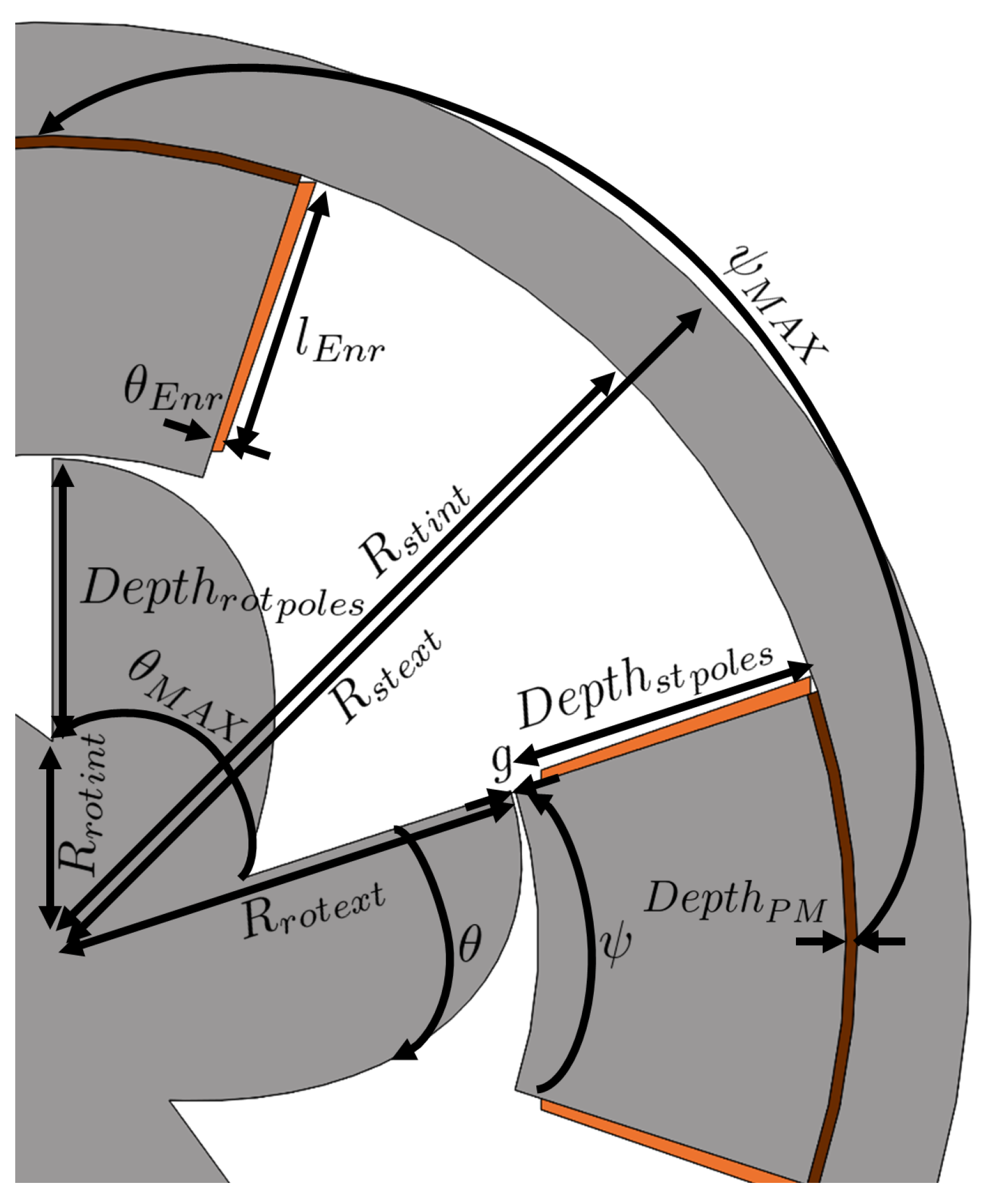
Figure 2.
Representation of the geometry of the DSPM S4R5 machine that shows the materials used with a zoom-in PM.
Figure 2.
Representation of the geometry of the DSPM S4R5 machine that shows the materials used with a zoom-in PM.

Figure 3.
B-H curve of Silicon Steel NGO 35JN200.
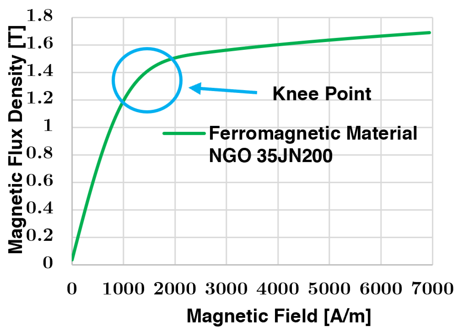
Figure 4.
Two-dimensional plane of DSPM S4R5 for illustration of PM flux direction and coil numbering.
Figure 4.
Two-dimensional plane of DSPM S4R5 for illustration of PM flux direction and coil numbering.
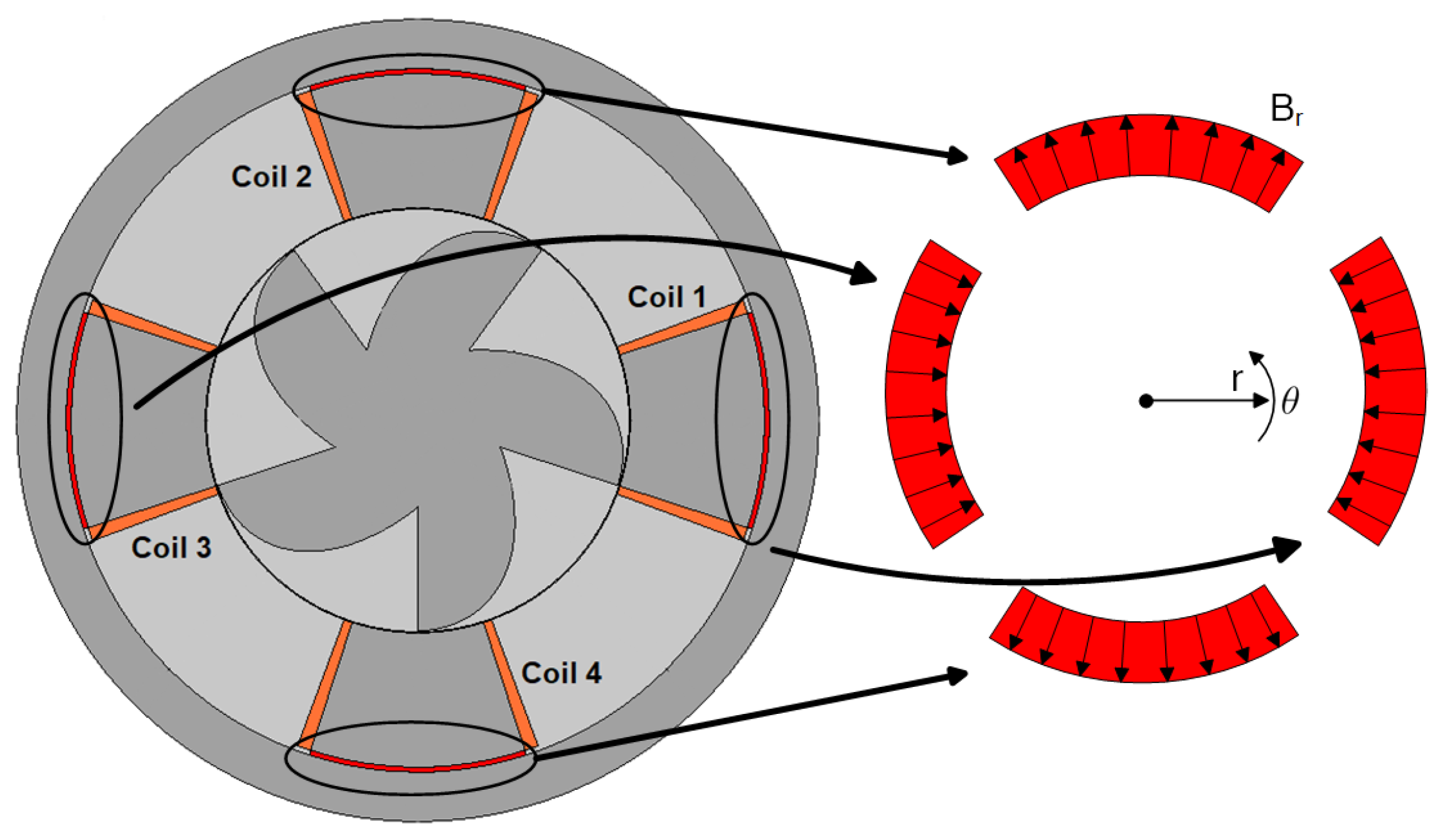
Figure 5.
Iron losses 3D graphic representation for the frequency and magnetic flux density values range where the most significant harmonics will be present.
Figure 5.
Iron losses 3D graphic representation for the frequency and magnetic flux density values range where the most significant harmonics will be present.
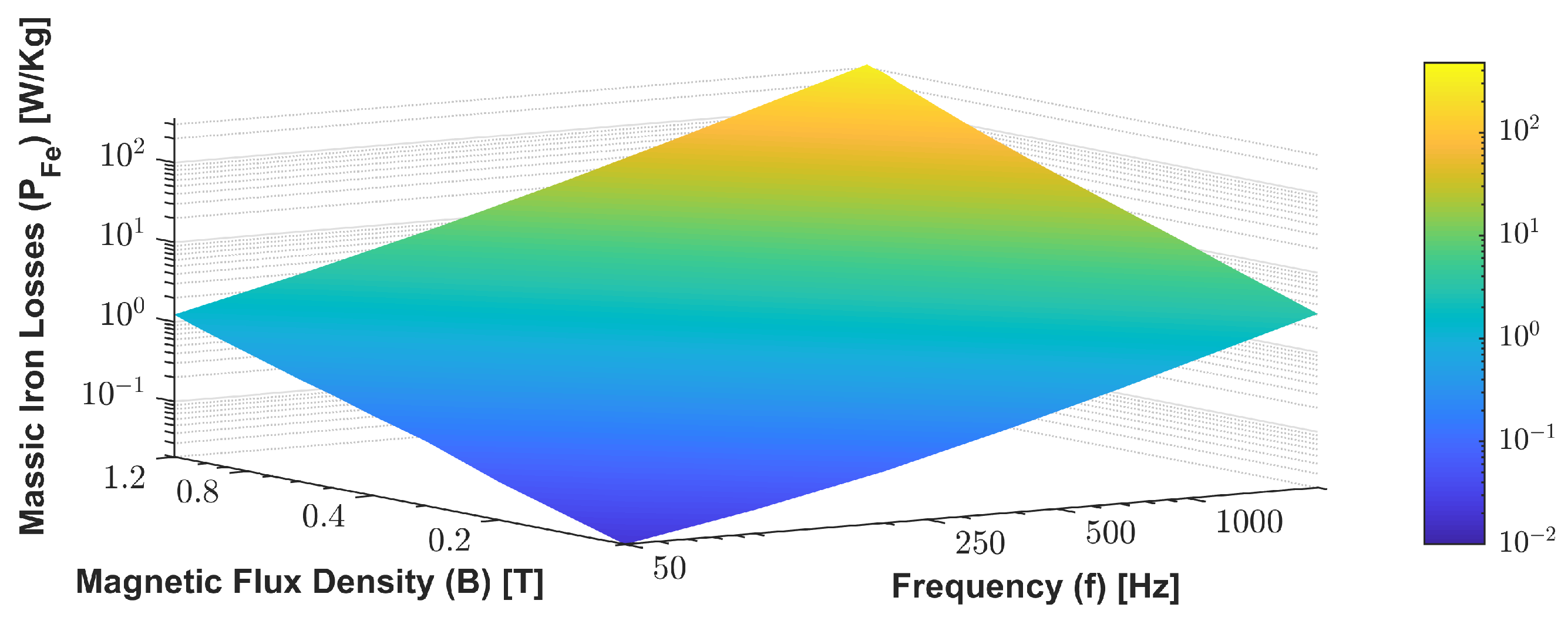
Figure 6.
NSGA-II and FEM procedure for DSPM S4R5 machine optimization. Adapted from [16].
Figure 6.
NSGA-II and FEM procedure for DSPM S4R5 machine optimization. Adapted from [16].
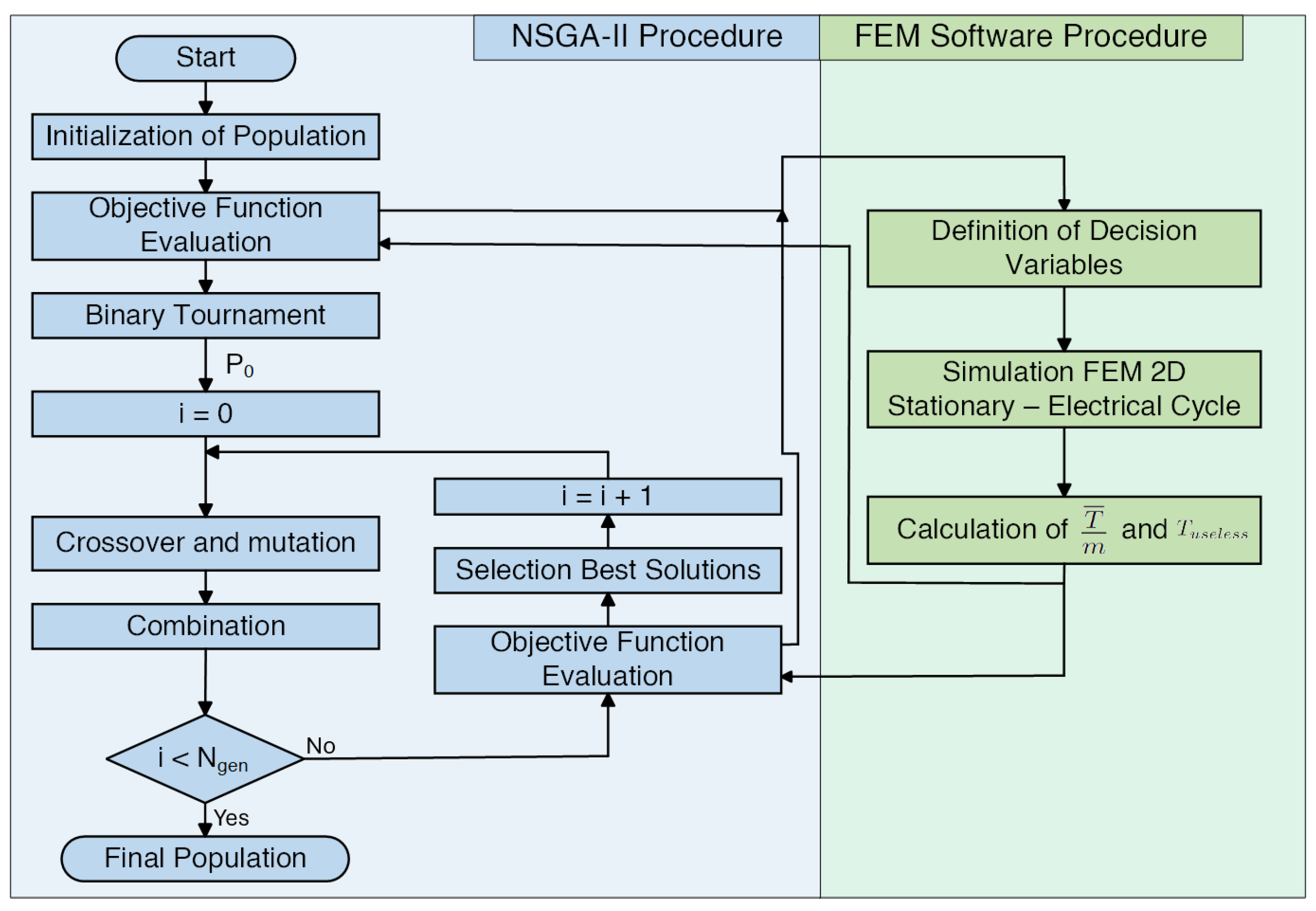
Figure 7.
Illustration of 3D complete geometry and a half-cross-cut plane of 3D entire geometry.
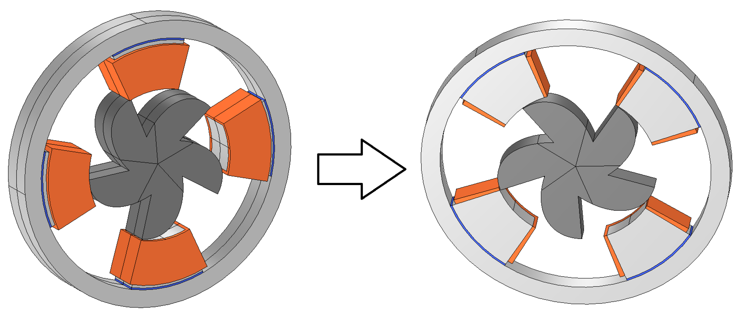
Figure 8.
Two-dimensional geometric representation of DSPM S4R5.
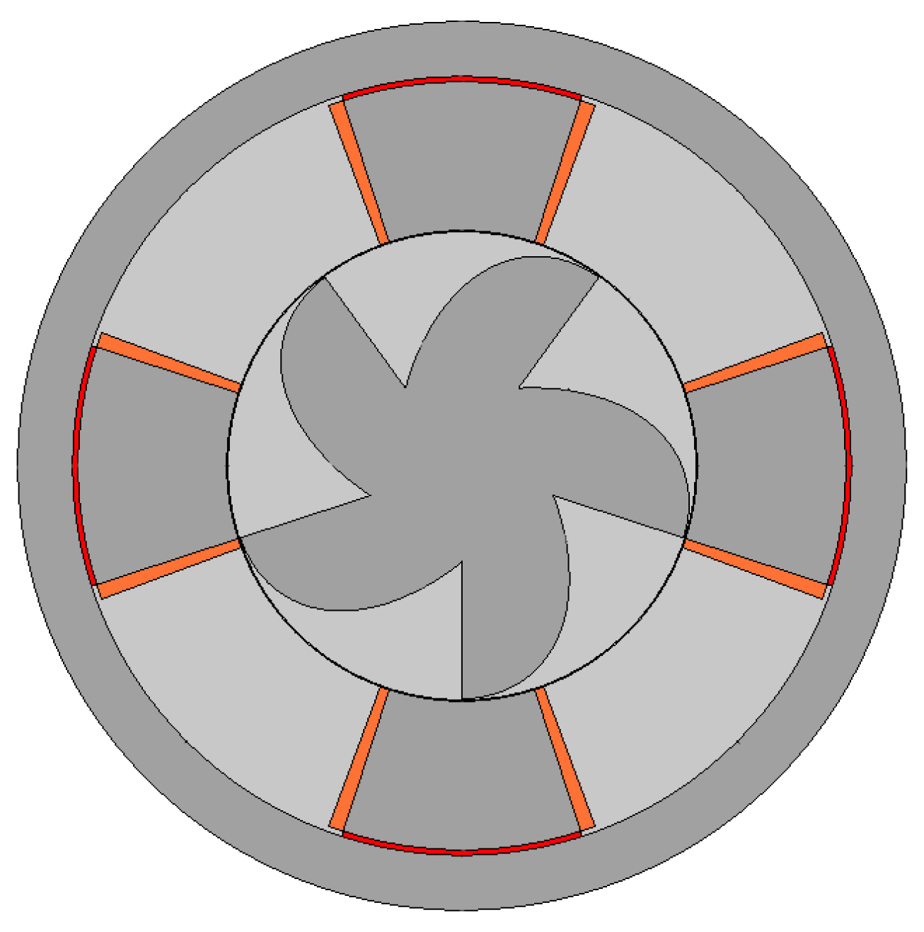
Figure 9.
Linked flux results for 2D geometry and 3D geometry.
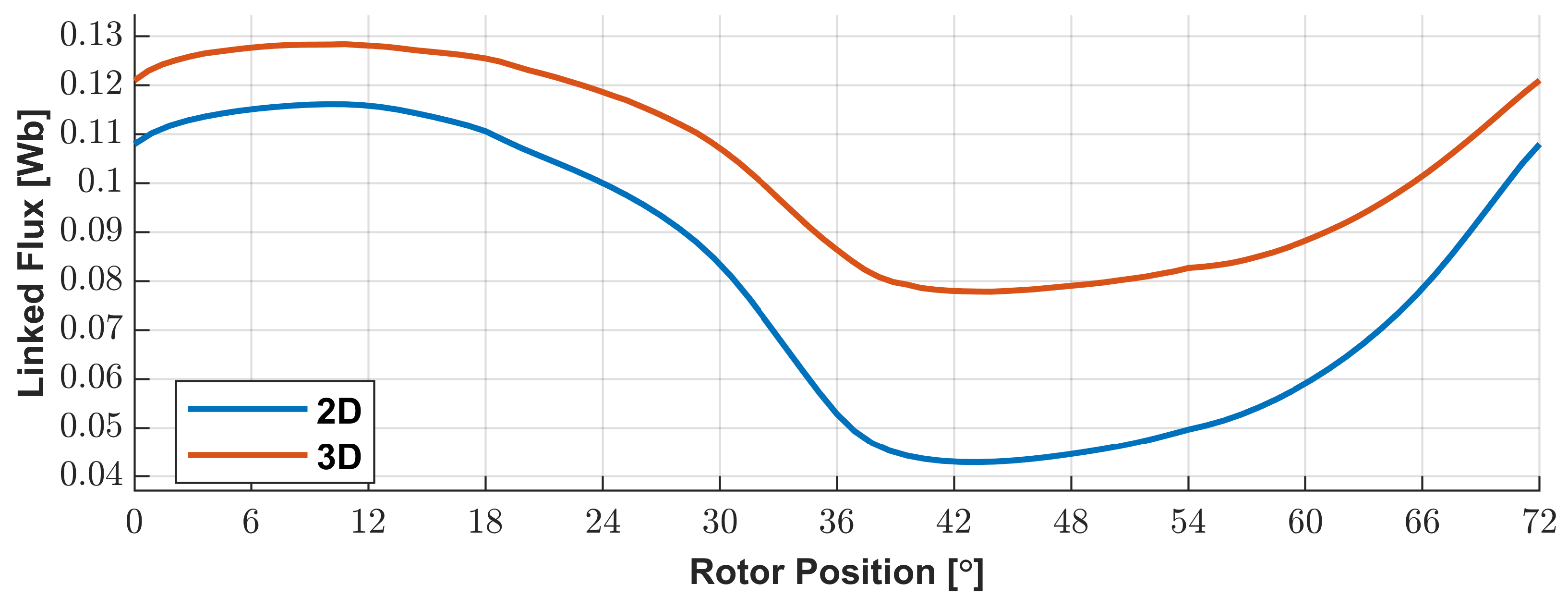
Figure 10.
Torque results for 2D geometry and 3D geometry.
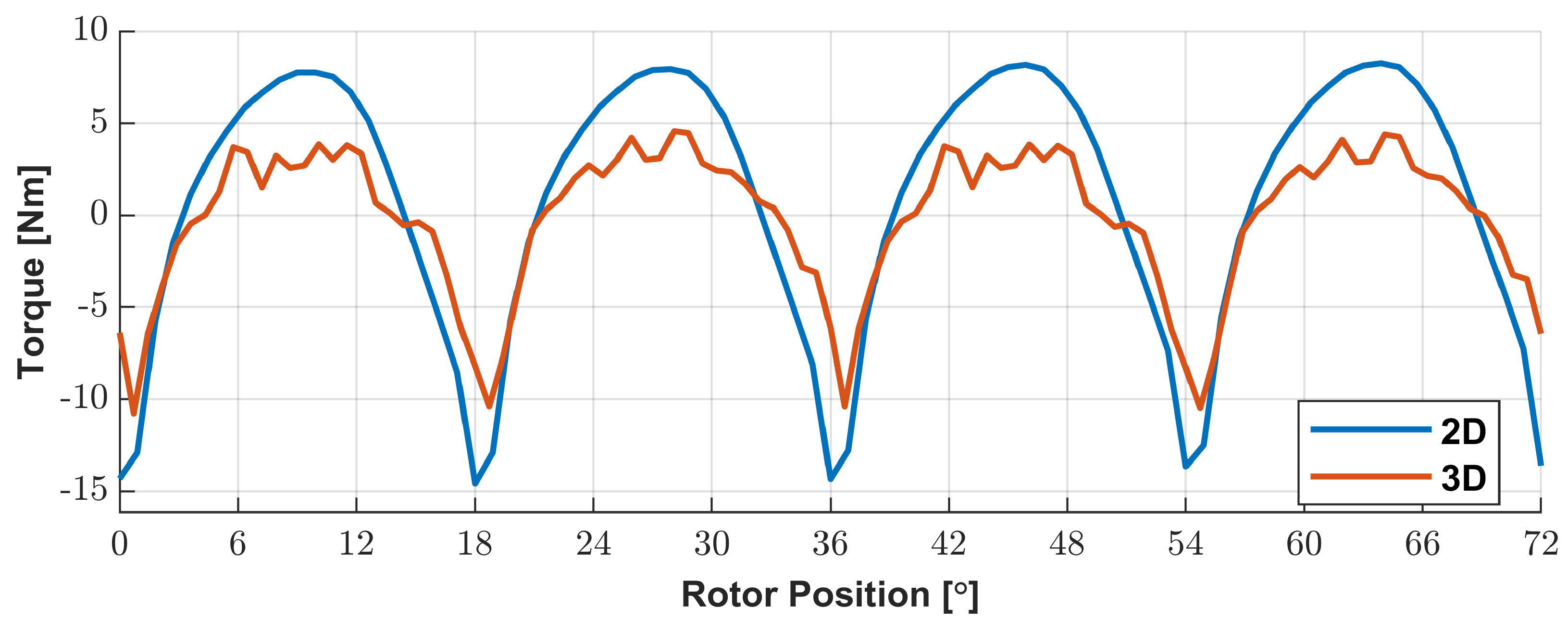
Figure 11.
Inductance maps: (a) self-inductance of coil 1; (b) mutual inductance of coil 2 with regard to phase current of coil 1; (c) inductance of coil 3 with regard to phase current of coil 1; (d) inductance of coil 4 with regard to phase current of coil 1.
Figure 11.
Inductance maps: (a) self-inductance of coil 1; (b) mutual inductance of coil 2 with regard to phase current of coil 1; (c) inductance of coil 3 with regard to phase current of coil 1; (d) inductance of coil 4 with regard to phase current of coil 1.
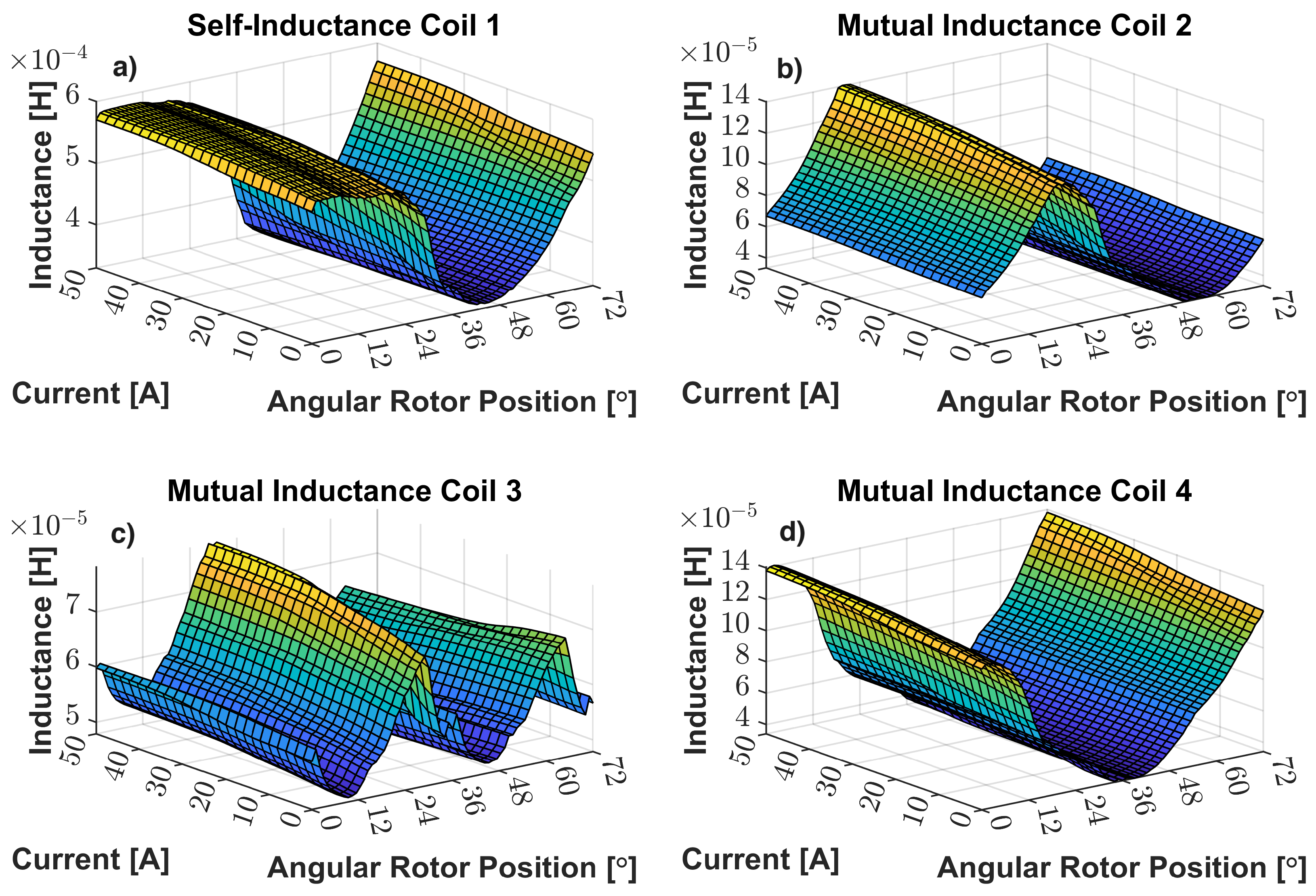
Figure 12.
N Parameter map: (a) N of coil 1; (b) N of coil 2; (c) N of coil 3; (d) N of coil 4.
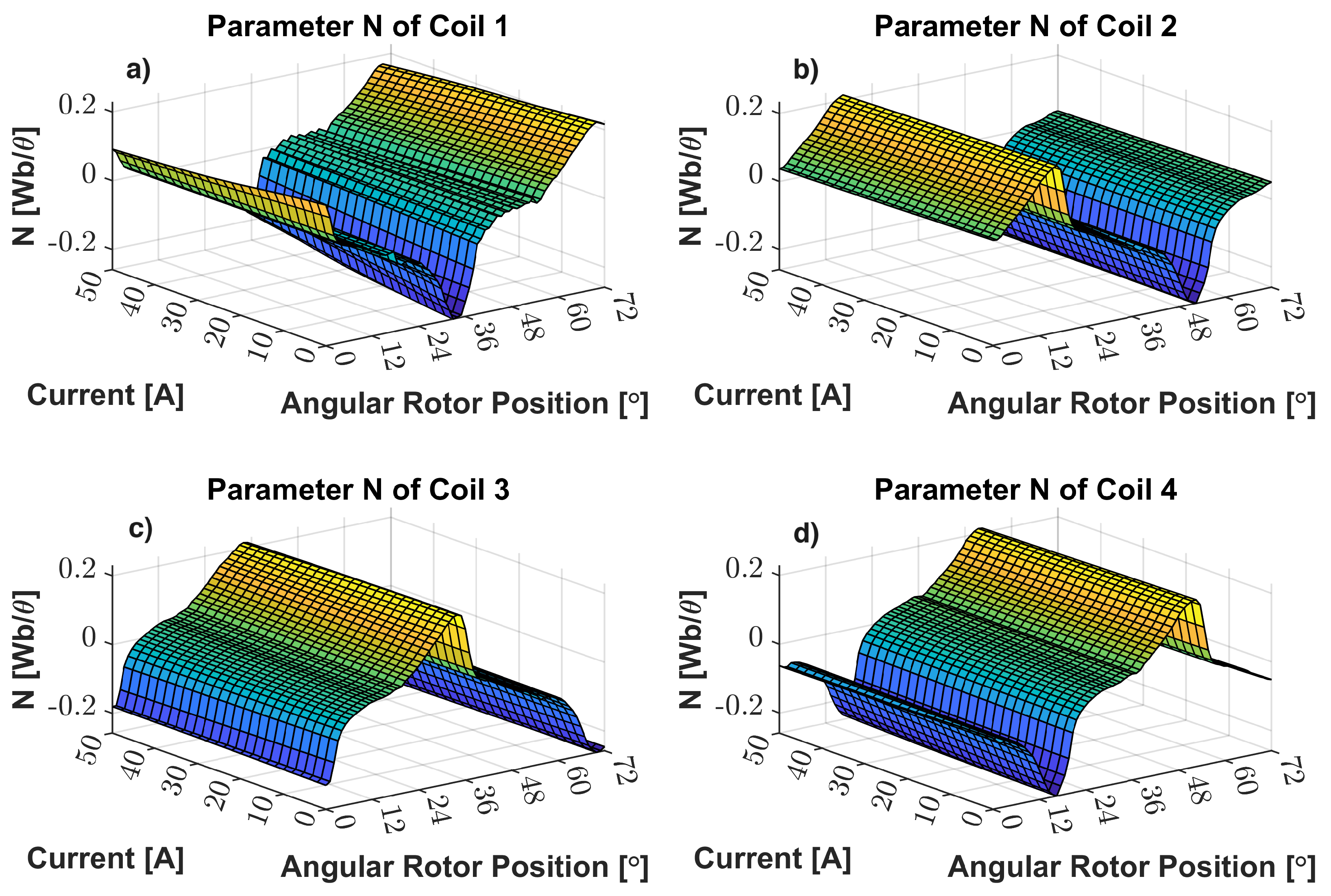
Figure 13.
Different current waveforms used to obtain the best current waveform regarding input torque mean value and oscillatory torque.
Figure 13.
Different current waveforms used to obtain the best current waveform regarding input torque mean value and oscillatory torque.
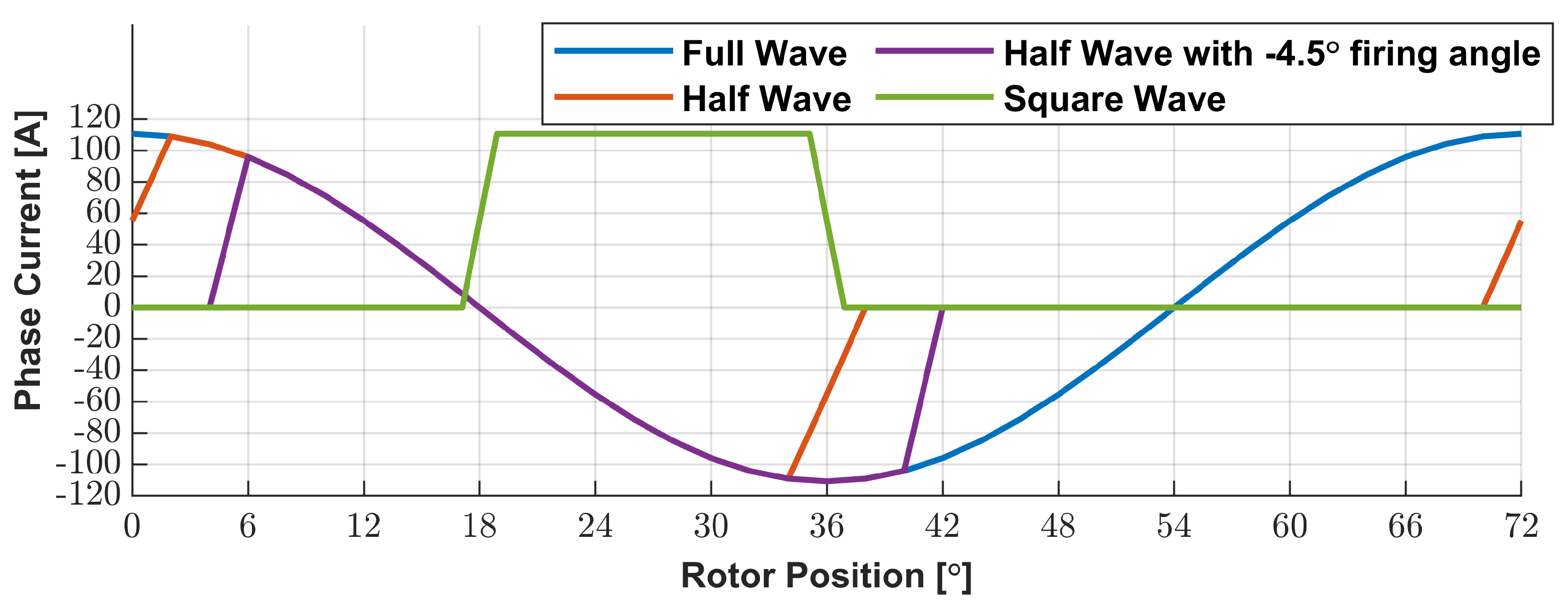
Figure 14.
Pareto curve obtained for the optimization process (in left part) and the optimal geometry selected from the point shown in the Pareto curve (in right part).
Figure 14.
Pareto curve obtained for the optimization process (in left part) and the optimal geometry selected from the point shown in the Pareto curve (in right part).

Figure 15.
Torque evolution of the results of optimized DSPM S4R5.
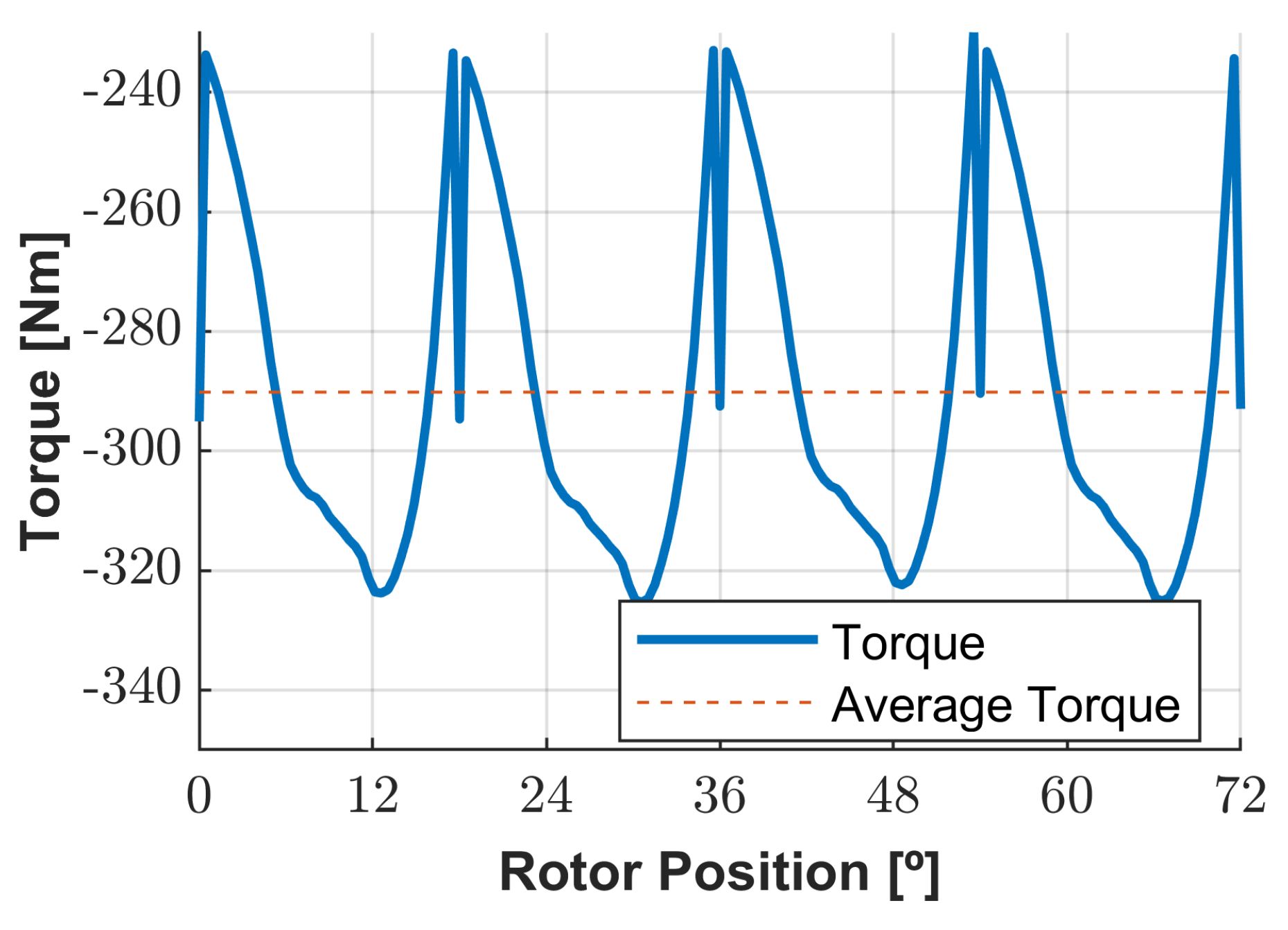
Figure 16.
Magnetic flux evolution of the results of optimized DSPM S4R5.
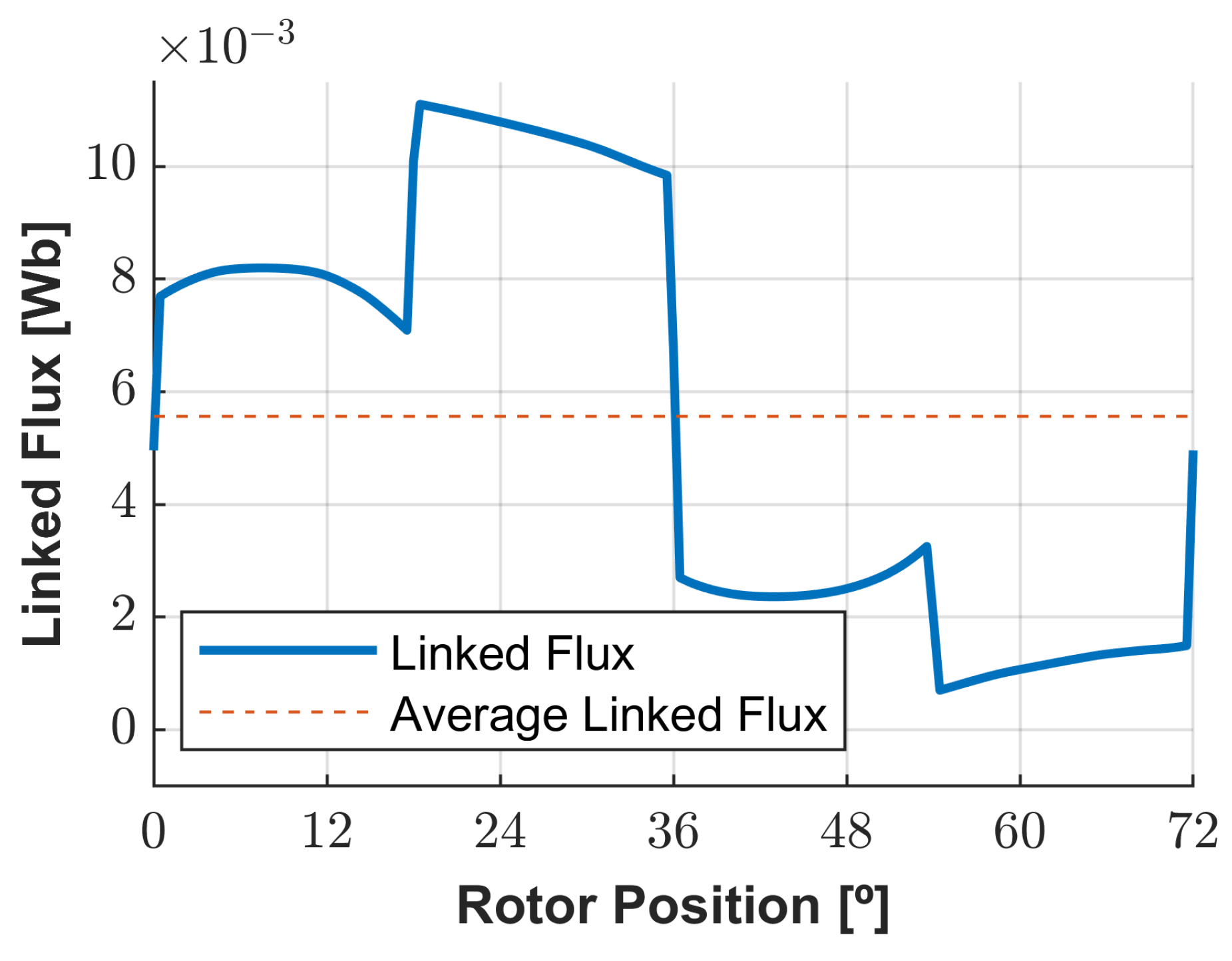
Figure 17.
Electromagnetic torque evolution of the 3D geometry of the optimized DSPM S4R5 in same load condition as optimization process.
Figure 17.
Electromagnetic torque evolution of the 3D geometry of the optimized DSPM S4R5 in same load condition as optimization process.
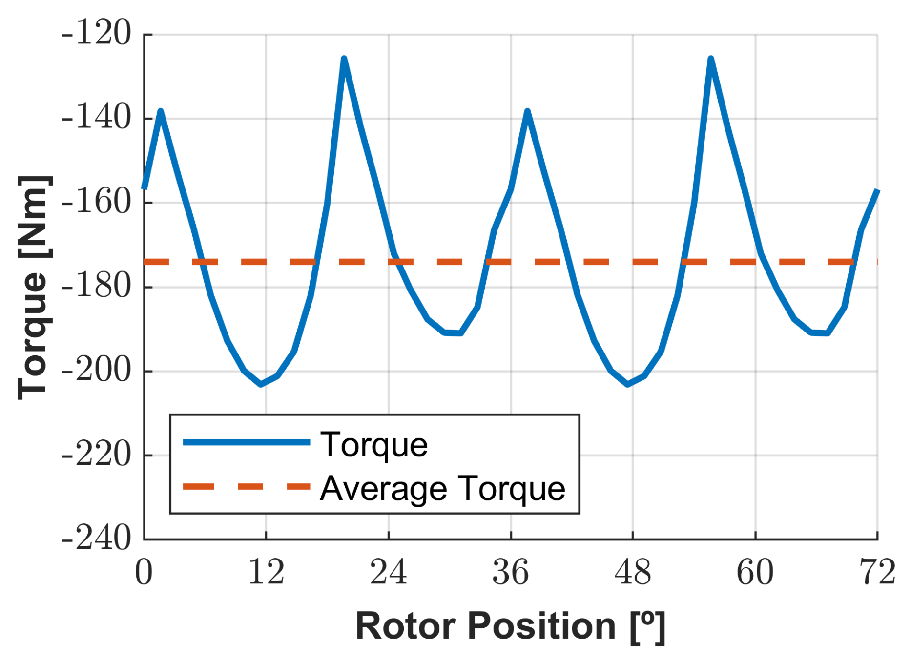
Figure 18.
Magnetic flux evolution of the 3D geometry of the optimized DSPM S4R5 in same load condition as optimization process.
Figure 18.
Magnetic flux evolution of the 3D geometry of the optimized DSPM S4R5 in same load condition as optimization process.
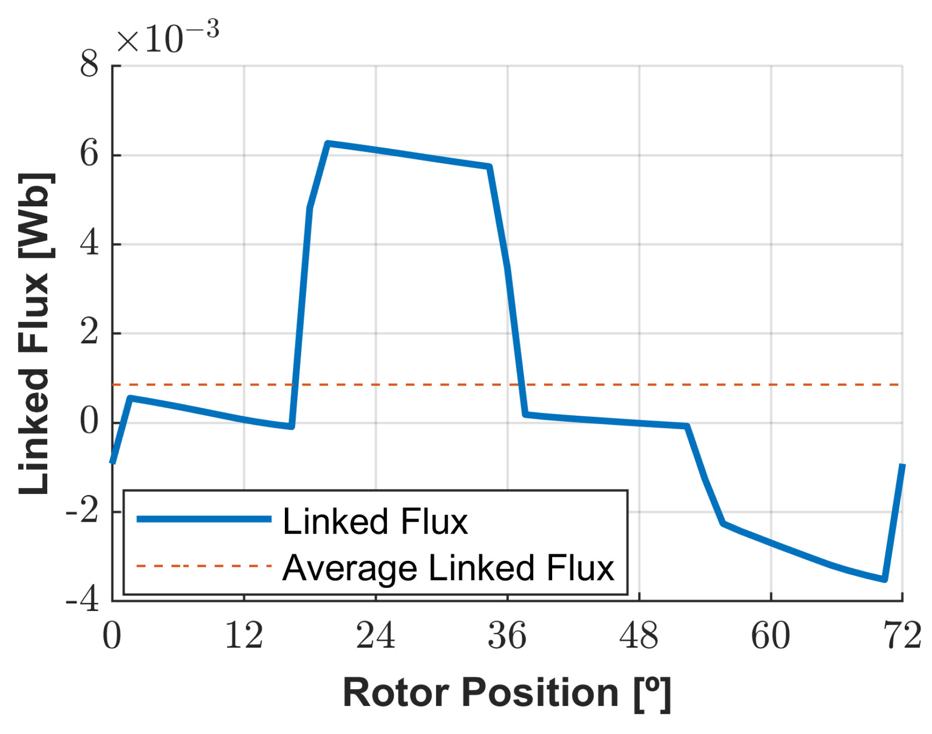
Figure 19.
Evolution of the generator voltages imposed by the ideal phase current waveforms.

Figure 20.
Evolution of the generator ideal phase current waveforms.
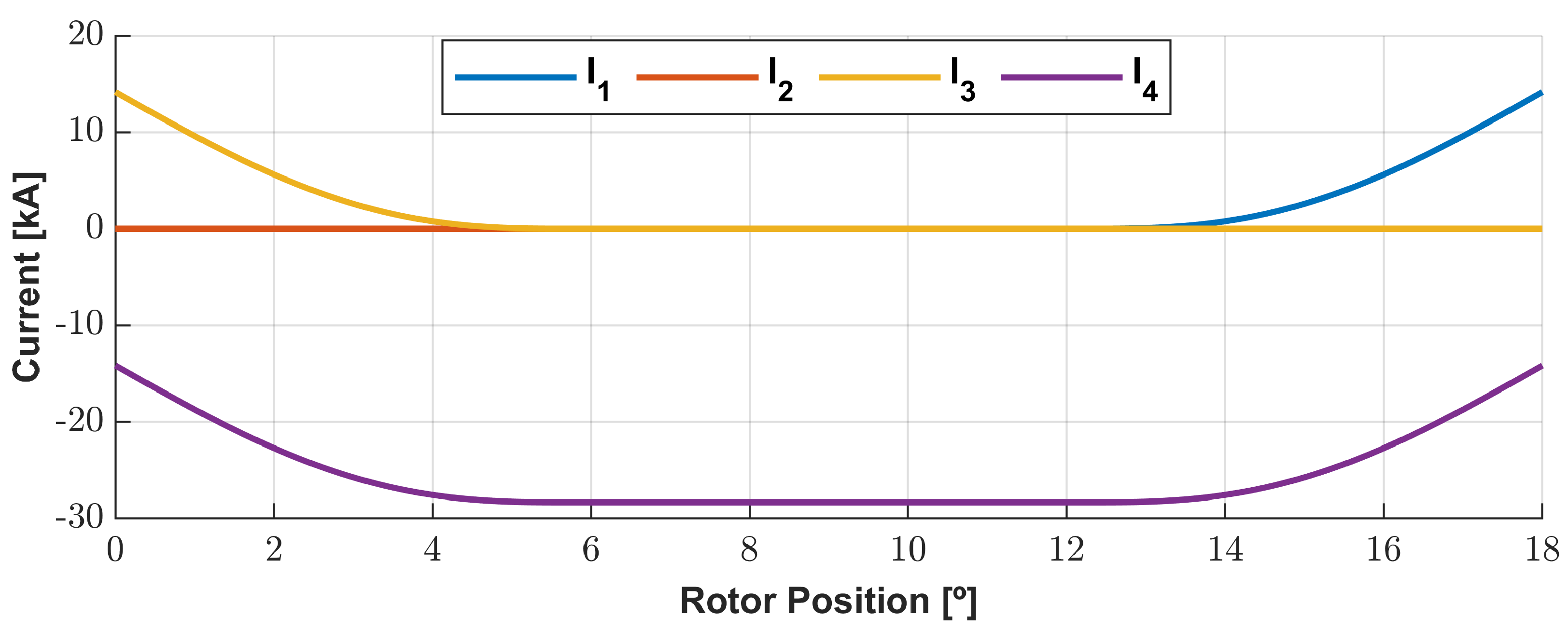
Figure 21.
Evolution of the total generator instantaneous power feeding the ideal phase current waveforms.
Figure 21.
Evolution of the total generator instantaneous power feeding the ideal phase current waveforms.
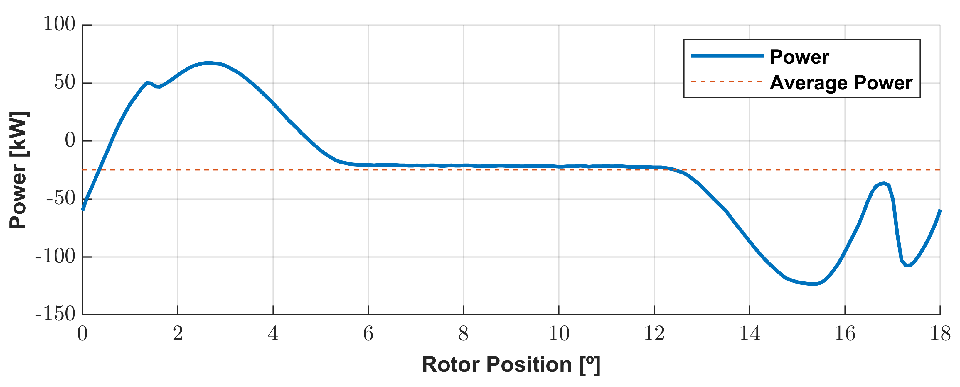
Figure 22.
Illustration of the initial 3D geometry.

Figure 23.
Illustration of the optimized 3D geometry.

Figure 24.
Linked flux results for initial geometry and optimized geometry for no-load condition.
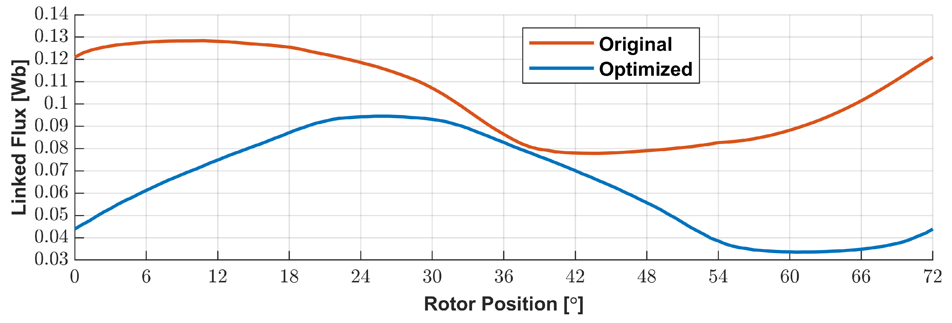
Figure 25.
Torque results for initial geometry and optimized geometry for no-load condition.
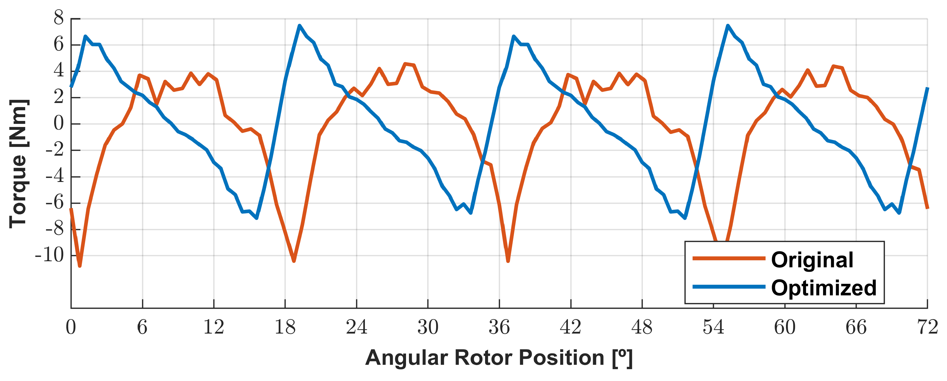
Figure 26.
Inductance maps: (a) self-inductance of coil 1; (b) mutual inductance of coil 2 with regard to phase current of coil 1; (c) inductance of coil 3 with regard to phase current of coil 1; (d) inductance of coil 4 with regard to phase current of coil 1.
Figure 26.
Inductance maps: (a) self-inductance of coil 1; (b) mutual inductance of coil 2 with regard to phase current of coil 1; (c) inductance of coil 3 with regard to phase current of coil 1; (d) inductance of coil 4 with regard to phase current of coil 1.
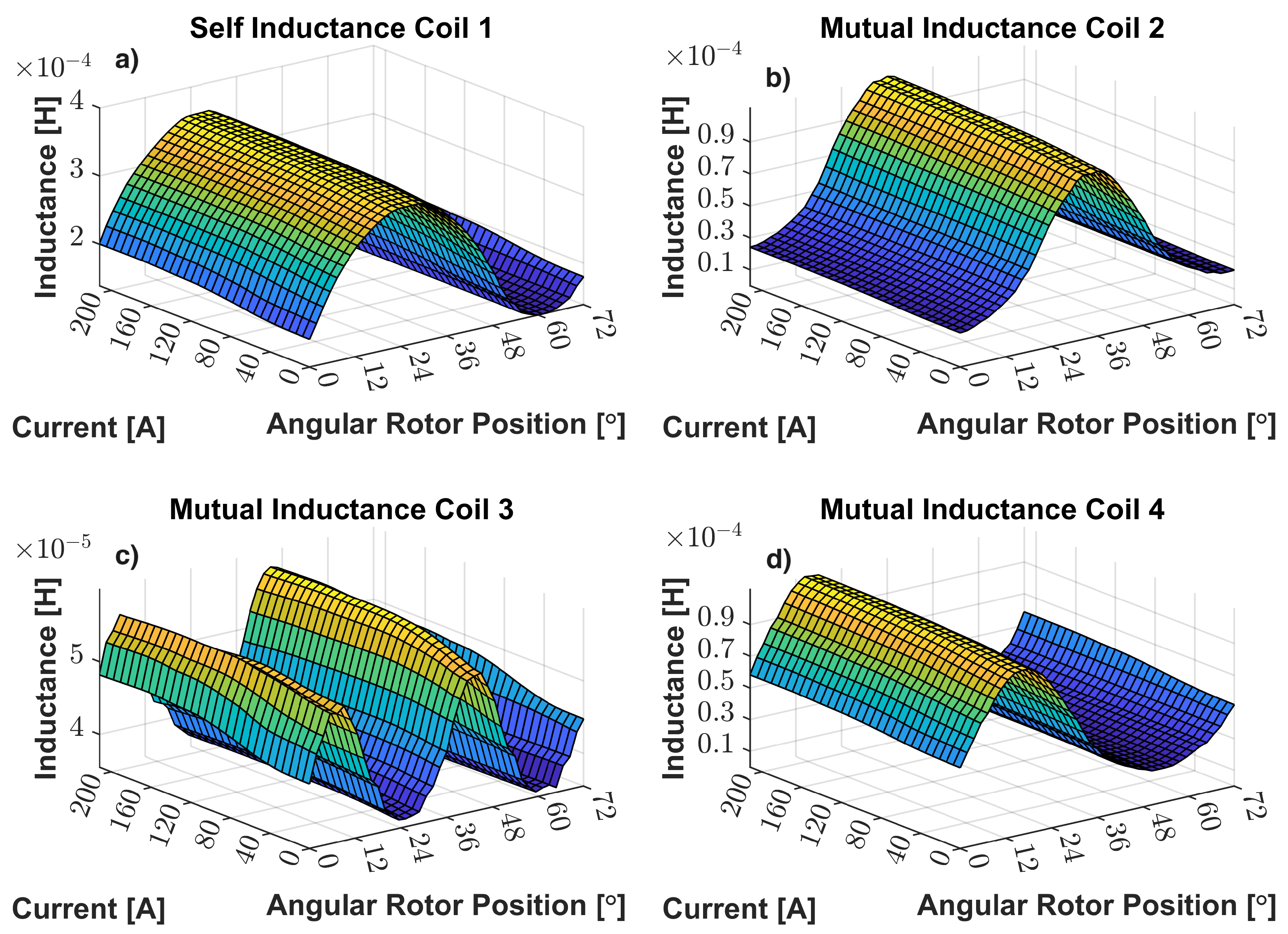
Figure 27.
N Parameter map: (a) N of coil 1; (b) n of coil 2; (c) n of coil 3; (d) n of coil 4.
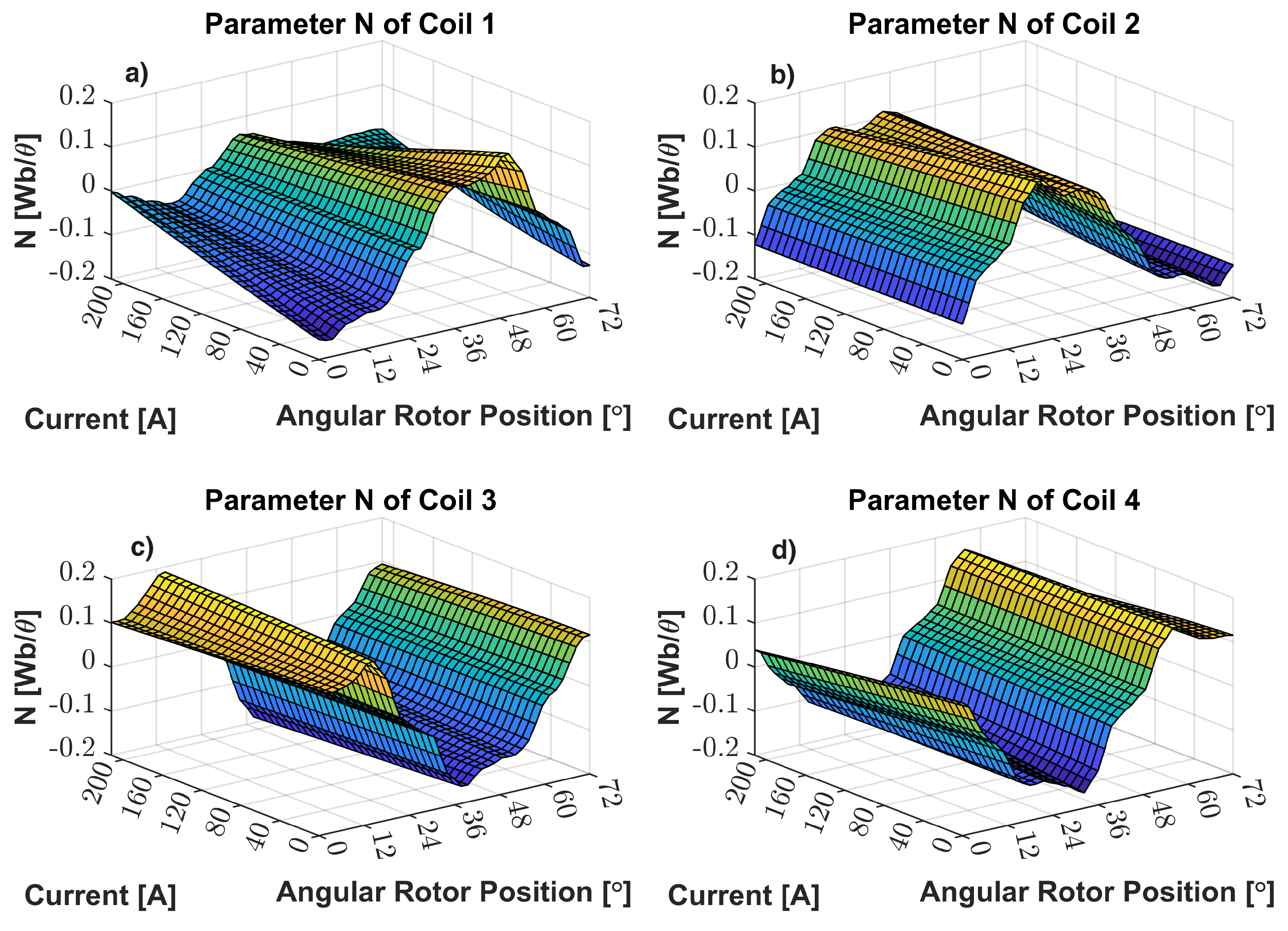
Figure 28.
Evolution of the generator voltages imposed on the AC/DC converter of the equivalent electric aircraft system.
Figure 28.
Evolution of the generator voltages imposed on the AC/DC converter of the equivalent electric aircraft system.
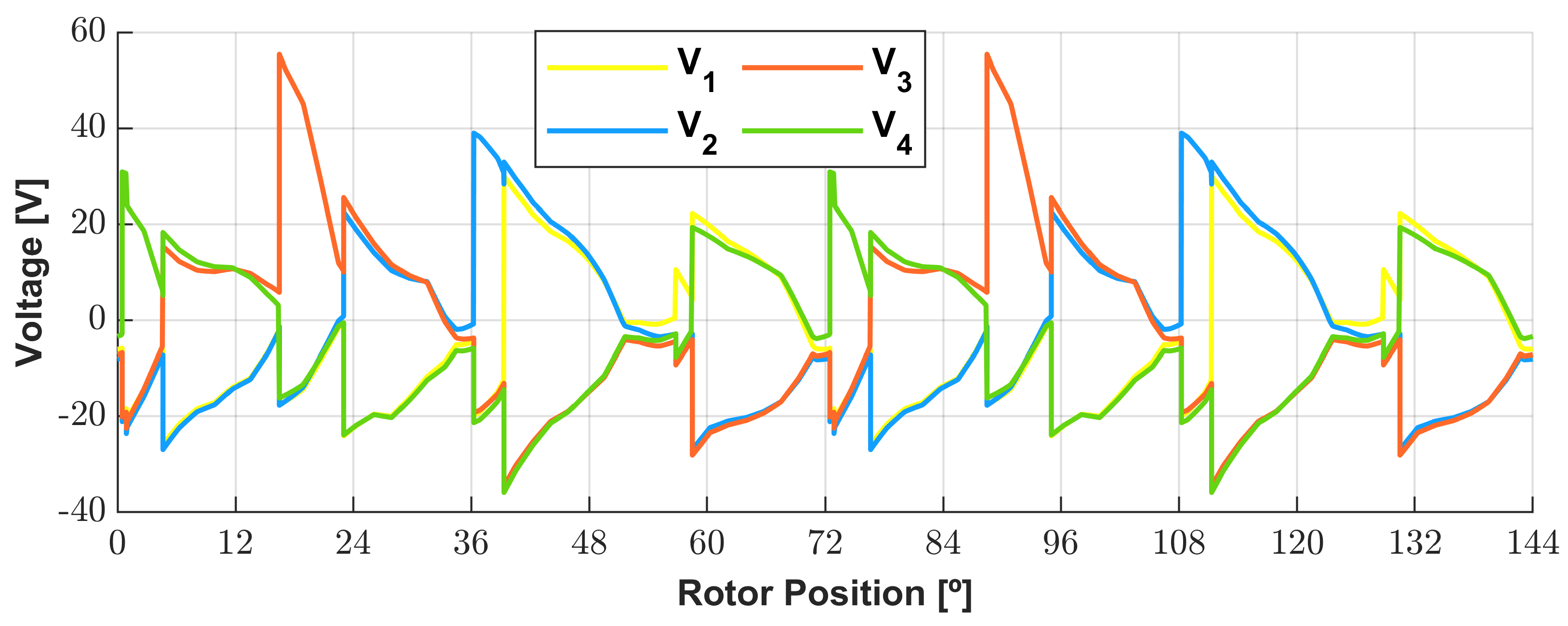
Figure 29.
Evolution of the generator currents feeding the AC/DC converter of the equivalent electric aircraft system.
Figure 29.
Evolution of the generator currents feeding the AC/DC converter of the equivalent electric aircraft system.
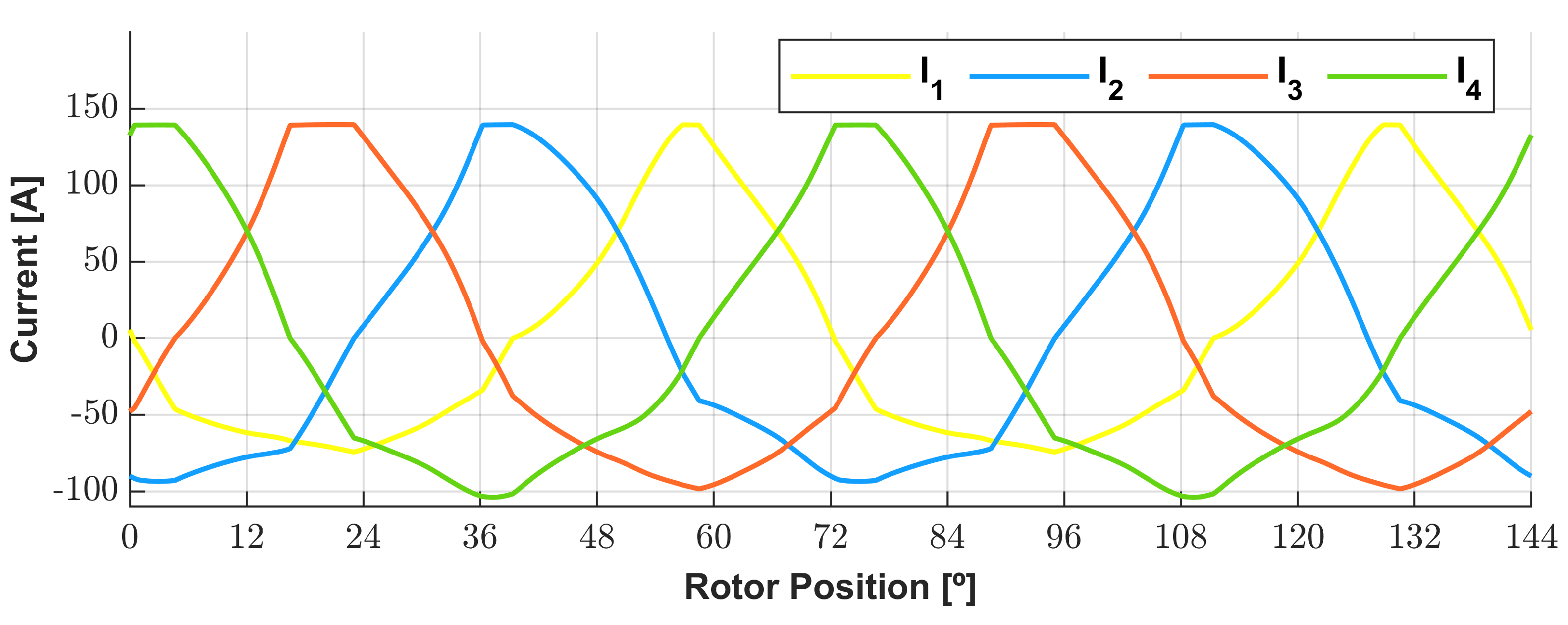
Figure 30.
Evolution of the generator output instantaneous power feeding the AC/DC converter of the equivalent electric aircraft system.
Figure 30.
Evolution of the generator output instantaneous power feeding the AC/DC converter of the equivalent electric aircraft system.

Table 1.
Geometric parameter values.
| Parameter | Description | Dimension |
|---|---|---|
| External radius of ring stator | 324 [mm] | |
| Internal radius of ring stator | 284 [mm] | |
| External radius of rotor | 170 [mm] | |
| Internal radius of rotor | 70 [mm] | |
| Depth of stator poles | 112.4 [mm] | |
| Depth of rotor poles | 100 [mm] | |
| Depth of PMs | 4 [mm] | |
| g | Airgap distance | 1.6 [mm] |
| Rotor pole angle | 36° | |
| Stator pole angle | 36° | |
| Rotor pole pitch | ||
| Stator pole pitch | ||
| Winding length | 100 [mm] | |
| Winding aperture angle | 0.04 [rad] | |
| DSPM total length | 80 [mm] |
Table 2.
Lower and upper limits of design variables used to optimize DSPM S4R5 machine.
| Design Variable | Lower and Upper Limits |
|---|---|
| 240–290 [mm] | |
| 135–155 [mm] | |
| 70–90 [mm] | |
| 50–110 [mm] | |
| 4–50 [mm] | |
| g | 1.95–2.2 [mm] |
| 0.05–0.45 [rad] | |
| 55–70 [mm] | |
| 0.25–0.65 [rad] | |
| 0.5–0.8 [rad] | |
| 170–220 [mm] | |
| −0.1–0.1 [rad] | |
| 0.2–0.6 | |
| 0.2–0.7 | |
| 0.4–1 |
Table 3.
Current waveform results in terms of electromagnetic torque mean value and oscillatory torque.
Table 3.
Current waveform results in terms of electromagnetic torque mean value and oscillatory torque.
| Current Waveform | [Nm] | [Nm] | |
|---|---|---|---|
| Cosine wave | |||
| Half-cosine | |||
| Half-cosine with firing angle | |||
| Square wave |
Table 4.
Geometric parameter values of the optimized DSPM S4R5 machine.
| Parameter | Dimension |
|---|---|
| [mm] | |
| [mm] | |
| [mm] | |
| [mm] | |
| 4 [mm] | |
| g | [mm] |
| [rad] | |
| [mm] | |
| [rad] | |
| [rad] | |
| [mm] | |
| [rad] | |
Disclaimer/Publisher’s Note: The statements, opinions and data contained in all publications are solely those of the individual author(s) and contributor(s) and not of MDPI and/or the editor(s). MDPI and/or the editor(s) disclaim responsibility for any injury to people or property resulting from any ideas, methods, instructions or products referred to in the content. |
© 2024 by the authors. Licensee MDPI, Basel, Switzerland. This article is an open access article distributed under the terms and conditions of the Creative Commons Attribution (CC BY) license (https://creativecommons.org/licenses/by/4.0/).
Share and Cite
MDPI and ACS Style
Neto, M.G.; da Silva, F.F.; Branco, P.J.d.C. Operational Analysis of an Axial and Solid Double-Pole Configuration in a Permanent Magnet Flux-Switching Generator. Energies 2024, 17, 1698. https://doi.org/10.3390/en17071698
AMA Style
Neto MG, da Silva FF, Branco PJdC. Operational Analysis of an Axial and Solid Double-Pole Configuration in a Permanent Magnet Flux-Switching Generator. Energies. 2024; 17(7):1698. https://doi.org/10.3390/en17071698
Chicago/Turabian StyleNeto, Manuel Garcia, Francisco Ferreira da Silva, and Paulo José da Costa Branco. 2024. "Operational Analysis of an Axial and Solid Double-Pole Configuration in a Permanent Magnet Flux-Switching Generator" Energies 17, no. 7: 1698. https://doi.org/10.3390/en17071698
Note that from the first issue of 2016, this journal uses article numbers instead of page numbers. See further details here.