Numerical Modeling of Non-Isothermal Laminar Flow and Heat Transfer of Paraffinic Oil with Yield Stress in a Pipe

Abstract

This paper presents the results of a study on the non-isothermal laminar flow and heat transfer of oil with Newtonian and viscoplastic rheologies. Heat exchange with the surrounding environment leads to the formation of a near-wall zone of viscoplastic fluid. As the flow proceeds, the transformation of a Newtonian fluid to a viscoplastic state occurs. The rheology of the Shvedoff–Bingham fluid as a function of temperature is represented by the effective molecular viscosity apparatus. A numerical solution to the system of equations of motion and heat transfer was obtained using the Semi-Implicit Method for Pressure-Linked Equations (SIMPLE) algorithm. The calculated data are obtained at Reynolds number Re from 523 to 1046, Bingham number Bn from 8.51 to 411.16, and Prandl number Pr = 45. The calculations’ novelty lies in the appearance of a “stagnation zone” in the near-wall zone and the pipe cross-section narrowing. The near-wall “stagnation zone” is along the pipe’s radius from r/R = 0.475 to r/R = 1 at Re = 523, Bn = 411.16, Pr = 45, u₁ = 0.10 m/s, t₁ = 25 °C, and t_w = 0 °C. The influence of the heat of phase transition of paraffinic oil on the development of flow and heat transfer characteristics along the pipe length is demonstrated.

1. Introduction

The non-isothermal laminar flow of high-viscosity fluid is of interest for the transition from a Newtonian state to a non-Newtonian (viscoplastic) state. This flow occurs in underground and submarine offshore main oil pipelines when pumping paraffinic oil [1].

The primary challenges in transporting this fluid through pipelines arise from its significant viscosity and yield stress, which strongly vary with temperature due to the presence of asphaltenes, paraffin, and resins [1,2,3,4]. Paraffinic oil behaves as a Newtonian fluid at high temperatures. However, at lower temperatures, the viscoplastic properties of a non-Newtonian fluid become evident [5,6]. Such oils have a high pour point (ranging from 12 to 30 °C). Heat exchange with the environment leads to changes in the physicochemical properties of the oil along the length of the pipe. The complex rheological characteristics of paraffinic oil are dictated by a pronounced escalation in plastic viscosity and yield stress as its temperature decreases [1].

Heat exchange with the surrounding environment can lead to the formation of a “stagnation zone” in the pipe, where the flow velocity equals zero [1,6,7]. The appearance of a stagnation zone can lead to two possible scenarios for the development of fluid flow with complex rheology [1,3]. When there is not enough kinetic and thermal energy in the flow, the stagnation zone coincides with the active cross-section of the pipeline. This leads to a sharp rise in hydraulic resistance, effectively causing the pipeline segment to “freeze” [2,3,5,6,7].

In the case of sufficient kinetic and thermal energy, the flow velocity increases when the pipe cross-section decreases, leading to the dissipation of the kinetic energy of the flow into thermal energy. The velocity of the flow increases from the wall towards the center of the pipe, consequently increasing the velocity gradient at the boundary of the flow—the stagnation zone. In this area, the fluid self-heats due to the released thermal energy, which directly depends on the square of the velocity gradient. [8,9]. In the theoretical limit, the flow transitions into a regime known as a “hydrodynamic thermal explosion” [8,9]. Heat losses along the pipe length are reduced due to the stagnant flow near its wall, acting as a kind of thermal insulation. In practice, the size of the stagnation zone is often stabilized [2,5].

A number of theoretical studies are devoted to the flow of a non-Newtonian Bingham fluid [10,11,12]. The content of the book [10] is a class of mathematical problems of physics and mechanics expressed through inequalities, problems with one-sided constraints, and thresholds or yield shear stress. One example of such problems is Bingham’s viscoplastic fluid with a yield shear stress [10].

The initial boundary value problem associated with the flow of a Bingham fluid is studied in [11]. The existence and uniqueness of a strong solution are proved under certain data assumptions. It is also shown that the solution exists global-in-time when the data are small and that the solution converges to a periodic solution if the external force is periodic in time [11].

A mathematical model describing the three-dimensional steady-state flow of a Bingham fluid in a bounded domain with threshold slip boundary conditions is studied in [12]. It is considered that flows can slide on solid surfaces when shear stresses reach a certain critical value. Using the variational inequality approach, a weak formulation of this problem is proposed. Sufficient conditions for the existence of weak solutions are established, and their energy estimates are given [12].

In the literature, there are several works on the study of heat transfer of such fluid for cases of flow in different geometries [13,14,15,16,17,18]. In [14], the results of laminar flow and the heat transfer of a viscoplastic fluid in a pipe are presented. However, the rheological properties of the viscoplastic fluid do not depend on temperature, and the influence of temperature on flow is not considered [14].

The present study, unlike [14], takes into account the dependence of plastic viscosity and yield stress on temperature. The system of equations for motion and energy is solved jointly, considering not only the dissipation of kinetic energy into heat but also the heat release due to the phase transition of paraffinic oil.

2. Mathematical Model

2.1. Physical Model of a Viscoplastic Fluid

A laminar flow of Newtonian fluid (paraffinic oil) flows into the pipe (see Figure 1). Then, it cools, spreading along the length of the pipe due to heat transfer through the pipe wall with the surrounding soil. The Reynolds number is determined by the fluid viscosity, which depends on the fluid temperature. The Reynolds number is Re = ρu₁R/µ_p1 = (0.5–1.2) × 10³ and the Prandtl number is Pr = µ₁C_P1/λ₁ = 45. The pipe has an inner diameter of D = 2R = 0.05 m and a length of L = 1 m (L/R = 40).

2.2. Rheological Properties of Non-Newtonian Fluid

The rheological model of the non-Newtonian fluid is determined using the concept of effective viscosity [19,20]. In the viscoplastic state, the effective viscosity ${\mu }_{eff}$ can be described by the Shvedoff–Bingham (SB) fluid model [21,22,23,24]. The SB model is a simple model of viscoplastic fluid, linearly combining yield shear stress and plastic viscosity. The effective molecular viscosity ${\mu }_{eff}$ of the SB fluid is expressed by the following formula [22,23,24]:

$${\mu }_{eff}=\left\{\begin{array}{ll}{\mu }_p+{\tau }_0{\left|\dot{\gamma }\right|}^{-1},& \mathrm{if} \left|\tau \right|>{\tau }_0\\ \infty ,& \mathrm{if} \left|\tau \right|\le {\tau }_0\end{array}\right.$$

(1)

where µ_P is the plastic viscosity, and τ₀ is the yield stress; $\dot{\gamma }=\sqrt{2S_{ij}{S}_{ij}}=S$ is the strain rate; $S_{ij}=0.5\left(\frac{\partial U_i}{\partial x_j}+\frac{\partial U_j}{\partial x_i}\right)$ is the shear rate tensor. If τ₀ = 0, then the fluid is Newtonian; if τ₀ > 0, then the fluid is an SB fluid. We use the strain rate tensor $\dot{\gamma }$as the shear rate.

The main difficulty in numerical modeling of viscoplastic flows with yield stress is associated with the presence of singular molecular viscosity in regions where the shear rate is zero. This difficulty is usually overcome by using regularization of the effective viscosity. In this study, we adopt the approach in [25], where the effective viscosity is approximated by a continuous function:

$${\mu }_{eff}={\mu }_p+{\tau }_0\frac{\left[1-\exp \left(-{10}^3\left|S\right|\right)\right]}{\left|S\right|}$$

(2)

2.3. The Basic Equations of Non-Newtonian Fluid Flow

The system of equations governing the motion and heat transfer of a steady laminar flow of a non-Newtonian fluid in a cylindrical coordinate system, accounting for (1), can be expressed as follows:

$$\frac{\partial (\rho u)}{\partial z}+\frac{1}{r}\frac{\partial }{\partial r}(r\rho v)=0$$

(3)

$$\rho \left(u\frac{\partial u}{\partial z}+v\frac{\partial u}{\partial r}\right)=-\frac{\partial p}{\partial z}+\left[\frac{\partial }{\partial z}\left(2{\mu }_{eff}\frac{\partial u}{\partial z}\right)+\frac{1}{r}\frac{\partial }{\partial r}\left({\mu }_{eff}r(\frac{\partial u}{\partial r}+\frac{\partial v}{\partial z})\right)\right]$$

(4)

$$\rho \left(u\frac{\partial v}{\partial z}+v\frac{\partial v}{\partial r}\right)=-\frac{\partial p}{\partial r}+\left[\frac{\partial }{\partial z}\left({\mu }_{eff}\left(\frac{\partial v}{\partial z}+\frac{\partial u}{\partial r}\right)\right)-\frac{2{\mu }_{eff}v}{r^2}+\frac{1}{r}\frac{\partial }{\partial r}\left(2r{\mu }_{eff}\frac{\partial v}{\partial r}\right)\right]$$

(5)

$$\frac{\partial \left(\rho c_{p}ut\right)}{\partial z}+\frac{\partial \left(\rho c_{p}vt\right)}{\partial r}=\frac{\partial }{\partial z}\left(\lambda \frac{\partial t}{\partial z}\right)+\frac{1}{r}\frac{\partial }{\partial r}\left(\lambda r\frac{\partial t}{\partial r}\right)+2{\mu }_{eff}\left[{\left(\frac{\partial u}{\partial z}\right)}^2+{\left(\frac{\partial v}{\partial r}\right)}^2+{\left(\frac{v}{r}\right)}^2+{\left(\frac{\partial u}{\partial r}+\frac{\partial v}{\partial z}\right)}^2\right]$$

(6)

where u and v are the velocity components of the fluid, respectively; z and r are the axial and radial coordinates, respectively; p and t are the pressure and temperature, respectively; ρ, c_p, and λ denote the density, specific heat capacity, and thermal conductivity of paraffinic oil, respectively.

2.4. Influence of Temperature on Non-Newtonian Fluid Properties

Decreasing the temperature of the oil can induce the crystallization of the paraffin it contains, leading to the release of phase transition heat. The total latent heat H can be determined by employing the apparent heat capacity method [26,27]:

$$c_P=\left\{\begin{array}{ll}{c}_S, t<t_S,& \mathrm{in} \mathrm{the} \mathrm{solid} \mathrm{phase}\\ c_{Int}, t_S\le t\le t_L,& \mathrm{in} \mathrm{the} \mathrm{transitional} \mathrm{zone}\\ c_L, t>t_L,& \mathrm{in} \mathrm{the} \mathrm{liquid} \mathrm{phase}\end{array}\right.$$

(7)

where c_S, c_L, and $c_{Int}=\left\{{\displaystyle \underset{t_S}{\overset{t_L}{\int }}{c}_L(t)dt+\chi H_{1\to 2}}\right\}/\left(t_L-t_S\right)$ represent the heat capacities of paraffin in solid, liquid, and transition states, respectively; t_L and t_S are the initial and final temperatures of paraffin formation in the oil flow, respectively; χ denotes the paraffin content in the oil; H_1→2 is the specific enthalpy of the phase transition of paraffin. In the system (7), t_L and t_S are the initial and final temperatures of paraffin formation in the oil flow: t_L = 25 °C; t_S = 15 °C; H_1→2 = 220.0 kJ/kg; χ = 0.15 or χ = 0.30.

Experimental data on the dependency of heat capacity c_L, plastic viscosity μ_P, and yield stress τ₀ of the paraffinic oil on temperature are described by empirical formulas:

$$c_L(t)=\left(53357+107.2\cdot t\right)/\sqrt{{\rho }_{20}}, [\mathrm{J}/(\mathrm{kg}·°C\left)\right]$$

(8)

$${\mu }_P(t)=0.3585\cdot \exp \left(-0.1792\cdot t\right), [\mathrm{Pa}·\mathrm{s}]$$

(9)

$${\tau }_0(t)=589.56\cdot \exp \left(-0.567\cdot t\right), \left[\mathrm{Pa}\right]$$

(10)

In

Table 1. The dependence of yield stress and plastic viscosity of a viscoplastic fluid on temperature [1].

t, °C	T, K	τ0, Pa	μP, Pa·s
0	273	589.6	0.3585
5	278	34.62044	0.14634
10	283	2.03286	0.05974
15	288	0.11937	0.02438
20	293	0.00701	0.00995
25	298	4.1156 × 10−4	0.00406
30	303	2.41662 × 10−5	0.00166

, the values of the yield stress τ₀ and plastic viscosity μ_P vs. fluid temperature are given.

The density and thermal conductivity of paraffinic oil exhibit weak temperature dependence, so we consider them constant. Empirical Formulas (8)–(10) are used for closing the model.

The solution of the system of equations governing motion and heat exchange is conducted in dimensionless variables: <$\stackrel{-}{z}=z/R;\hspace{0.33em}\stackrel{-}{r}=r/R;U=u/u_1;V=v/u_1;$ $P=p/p{u}_1^2;$ $\theta =\left(t-t_w\right)/\left(t_1-t_w\right)$. Here, R is the radius of the pipe; u₁ represents the average flow velocity at the pipe inlet; t₁ and t_w denote the temperatures of the fluid at the pipe’s inlet and wall, respectively.

The regime parameters of the problem include the Reynolds number $\mathit{Re}=\rho u_{1}R/{\mu }_{p1}$ and the Prandtl number $\mathit{Pr}={\mu }_{p1}{c}_{p1}/{\lambda }_1$. The Bingham number $Bn={\tau }_{0w}R/{\mu }_{pw}{u}_1$ is determined by the values of yield stress and plastic viscosity at the pipe wall temperature.

2.5. Boundary Conditions

At the pipe wall, the conditions of no-slip are applied for the fluid velocity. For the temperature of the fluid flow at the wall, it is set equal to the temperature of the pipe wall:

$$\overline{r}=r/R=1: U=V=0, \theta =0$$

(11)

Symmetry conditions are imposed for all the flow variables at the axis of the pipe:

$$\overline{r}=r/R=0: \frac{\partial U}{\partial \overline{r}}=\frac{\partial V}{\partial \overline{r}}=\frac{\partial \theta }{\partial \overline{r}}=0$$

(12)

At the inlet section (z/R = 0), constant velocity and temperature were prescribed across the entire cross-section of the pipe:

$$\overline{z}=z/R=0: U=1, V=0, \theta =1.$$

(13)

At the outlet section (z = L), the derivatives of all sought parameters in the axial direction are set equal to zero:

$$\overline{z}=L/R: \frac{\partial U}{\partial \overline{z}}=\frac{\partial V}{\partial \overline{z}}=\frac{\partial \theta }{\partial \overline{z}}=0$$

(14)

Consequently, the set of Equations (1)–(14) with the input and boundary conditions forms a closed system of equations, enabling the calculation of all required variables.

3. Numerical Method

The system of equations governing motion and heat exchange is solved in the variables “velocity-pressure components” [28]. The finite volume method on the staggered grid was used to discretize the equations. The fields for u, v, p, and t had their own separate grids and, consequently, separate control volumes. For the convective terms of the differential equations, the power-law scheme recommended by Patankar [28] is applied. For diffusive flows, the second-order central differences of accuracy [29] are used.

The SIMPLE algorithm was used to solve the system of Equations (3)–(6), with each iteration consisting of the following steps

• Solve the discretized energy Equation (6) to determine the values of t_ij;
• Solving the discretized momentum Equations (4) and (5) to determine values of u_ij,v_ij;
• Compute the uncorrected mass fluxes at the surfaces. If their values are sufficiently small, stop the iterations of the SIMPLE algorithm (in this case, a solution is reached);
• Solve the pressure correction equation based on the continuity Equation (3) to obtain the cell values of the pressure correction (values of ∆p_ij);
• Update the pressure field: $p_{ij}^{k+1}=p_{ij}^k+{\alpha }_P·{∆p}_{ij}^k$, where ${\alpha }_P$ is the under-relaxation factor for pressure (0.005 ≤ ${\alpha }_P$ ≤ 0.5);
• Correct the cell values of u_ij and v_ij (procedure described by Patankar [28]).

Discretized forms of Equations (3)–(6) are systems of linear algebraic equations with respect to the values of ${∆p}_{ij}$, $u_{ij}$, $v_{ij}$, $T_{ij}$, respectively. These systems of linear equations were solved using the line-by-line method, a convenient combination of the Gauss–Seidel method and the direct method TDMA (for cells’ j-direction at a fixed value of i).

Numerical calculations were performed using our proprietary code. The convergence of the algorithm was tested on grids with the sizes of 750 × 50 and 1500 × 120 control volumes.

4. Discussion of Calculated Data

The non-isothermal flow of paraffinic oil in a pipe with an inner diameter of D = 2R = 0.05 m is considered. Calculations were performed along the length of the pipe for L/R ranging from 40 to 60. The average velocity of the paraffinic oil at the pipe inlet u₁ varied from 0.1 to 0.2 m/s, with its initial temperature set at t₁ = 25 °C. The pipe wall temperature was considered equal to the ambient temperature t_Soil, ranging from 0 to 10 °C. The density of the fluid at the inlet section was ρ₁ = 850 kg/m³.

4.1. Validation and Verification of Computational Data

For the verification of calculations, the known results of the laminar flow of SB fluid can be used. The calculated data [30] of the radial distribution of dimensionless axial velocity (a) and dynamic viscosity (b) across the pipe section are depicted in Figure 2.

The calculations were conducted for two mixing fluids—one being a Newtonian fluid moving in the central part of the pipe (R₁/R ≤ 0.55), while a ring flow of Shvedoff–Bingham fluid is introduced in the near-wall part (R₂/R = (R₁ + q)/R = 0.65 – 1). The intermediate mixing layer between the Newtonian and SB fluids has a thickness of q/R = 0.1. It should be noted that in this instance, the mathematical model was adjusted by incorporating a diffusion equation with a Schmidt number Sc = μ₁/(ρ₁D_S) = 10 based on data from [30]. Here, subscripts “1” and “2” denote the Newtonian and SB fluids, respectively, and D_S is the coefficient of molecular diffusion. Comparisons were conducted between an isothermal laminar flow regime of Newtonian fluid (1) and SB fluid with a specified Bingham number $Bn={\tau }_{0}R/\left({\mu }_1{u}_1\right)$ = 5 (2). A notable quantitative agreement can be observed between the data obtained from our numerical calculations and the findings reported in [29].

Figure 3 illustrates radial distributions of dimensionless longitudinal velocity and temperature across the pipe section ${\theta }_m=(t_w-t)/(t_w-t_m)$ for the laminar flow and heat transfer of the SB fluid [14].

Comparisons were made under conditions Y = τ₀R/(μ_Pu₁) = 0 (Newtonian fluid, curve 1) and Y = 1.99 (SB fluid, curve 2) with a Reynolds number of Re₁ = ρRu₁/μ_P = 25. For the Newtonian fluid, a good agreement was achieved with the data from the calculation [14] across the entire pipe radius, both for axial velocity and fluid temperature. However, for the SB fluid, some discrepancy was observed between the results of our numerical calculations and the data from [14] in the region of y/R ≤ 0.5. Nevertheless, good agreement was obtained between our calculations and the data from [14] in the core flow region.

4.2. Computational Data for Non-Isothermal Laminar Flow in a Pipe

The computational data were obtained for Reynolds numbers $\mathit{Re}=\rho u_{1}R/{\mu }_{p1}$, ranging from 523 to 1046; Bingham numbers $Bn={\tau }_{0w}R/\left({\mu }_{pw}{u}_1\right)$, ranging from 8.51 to 411.16; and a Prandtl number $\mathit{Pr}={\mu }_{p1}{c}_{p1}/\lambda$ = 45.

Figure 4 illustrates profiles of axial velocity U, excess temperature θ across the radius at different sections, and pressure distribution along the length of the pipe under operating parameters Re = 523, Bn = 411.16, Pr = 45, u₁ = 0.10 m/s, t₁ = 25 °C, t_w = 0 °C. The appearance of the flow stagnation zone is evident, reaching from r/R = 0.475 to r/R = 1 at z/R = 30 (see Figure 4a). Subsequently, the thickness of this zone remains nearly unchanged, establishing a core of constant velocities characteristic of the viscoplastic flow of Shvedoff–Bingham fluid. This is apparent from the axial velocity U profile at z/R = 40 (see Figure 4a).

The profiles of excess temperature were obtained considering the heat dissipation from kinetic energy and phase transition during paraffin crystallization with parameters t_L = 25 °C, t_S = 15 °C, H_1→2 = 220.0 kJ/kg, χ = 0.15. The initial temperature of the paraffinic oil, θ = 1.0 (t₁ = 25 °C), gradually decreases to θ = 0.2 (t = 5 °C) along the axis of the pipe due to cooling (see Figure 4b). At t = 5 °C, the values of yield stress and plastic viscosity are ${\tau }_0=$ 34.62 Pa and μ_P = 0.146 Pa·s (see Table 1), indicating a viscoplastic state of the paraffinic oil.

The pressure distribution P exhibits a monotonic nonlinear variation along the length of the pipe (see Figure 4c). The transition from a Newtonian fluid to a viscoplastic state leads to an increase in dimensionless pressure up to P = 1850 (equivalent to p = 15,500 Pa) at the initial section for fluid pumping along the pipe length.

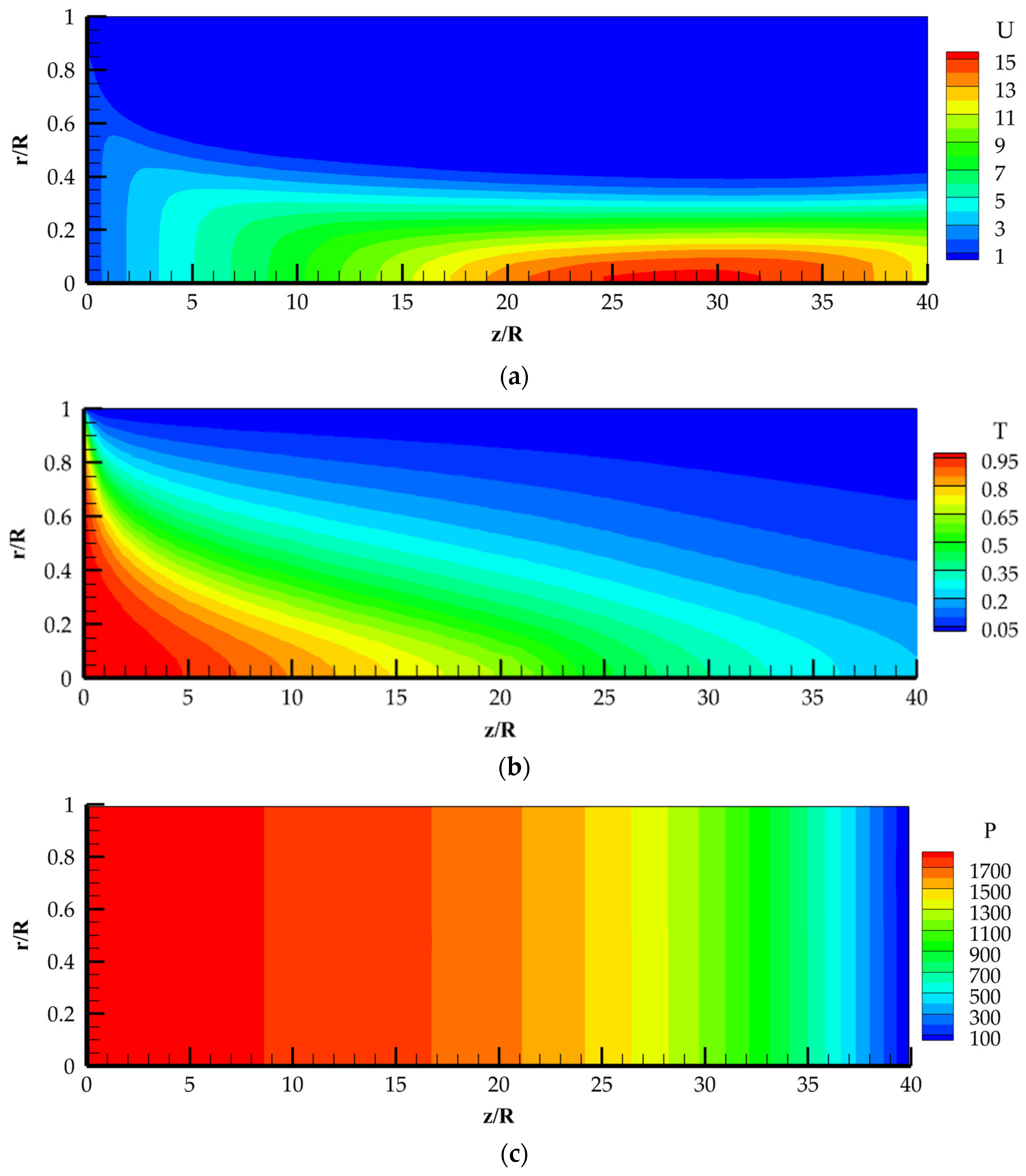
Contour plots of axial velocity U, excess temperature θ, and pressure P under these operational parameters are shown in Figure 5. The maximum value of axial velocity U is found in the interval from 24 to 32 along the length of the pipe z/R (see Figure 5a). Subsequently, the maximum value of axial velocity U decreases along the axis of the pipe from 15.55 to 11.85 (see Figure 4a). In the central zone, a core flow with constant velocity emerges. The contours of axial velocity U become nearly parallel at the outlet section of the pipe (see Figure 5a).

The contour of the maximum excess temperature θ sharply decreases in the initial section of the pipe, and subsequently, the decrease stabilizes somewhat (see Figure 5b). The contour of the minimum value of the excess temperature θ varies along the pipe length (see Figure 5b). This affects the thickness of the stagnation zone, which increases in the flow direction (see Figure 5a).

The contours of pressure P remain constant across the pipe section and decrease along the pipe length (see Figure 5c). Specifically, up to z/R = 8, the pressure P varies almost linearly, and thereafter, the decrease in P occurs nonlinearly.

Thus, contour plots of axial velocity U, excess temperature θ, and pressure P clearly describe, qualitatively and quantitatively, the non-isothermal laminar flow and heat transfer with the rheology of Newtonian and Shvedoff–Bingham viscoplastic fluid in the pipe.

The calculated data are obtained at the following regime parameters. u₁ = 0.10 m/s; t₁ = 25 °C; t_w = 5 °C; Re = 523; Bn = 59.14 are shown in Figure 6 and Figure 7.

The increase in the pipe wall, consequently decreasing the yield stress and plastic viscosity, affects the distribution of the axial velocity profile U, excess temperature θ, and pressure P. The maximum value of axial velocity on the pipe axis is U_m = 7.5 at z/R = 30 (see Figure 6a). The radius of the stagnation zone is r/R = 0.67, where the axial velocity is U = 0. Subsequently, the maximum value of axial velocity decreases to U_m = 4.5, and the radius of the stagnation zone increases to r/R = 0.77 at the outlet section of the pipe z/R = 40, i.e., the thickness of the stagnation zone slightly decreases.

The core flow with a constant velocity U = U_m, typical of viscoplastic flow, is visible at z/R = 40 (see Figure 6a).

Profiles of excess temperature θ (see Figure 6b) show a slight decrease along the pipe length compared to the previous case (see Figure 4b).

The distribution of pressure P shows a nonlinear decrease, which is explained by the fluid transition from Newtonian to viscoplastic (see Figure 6c).

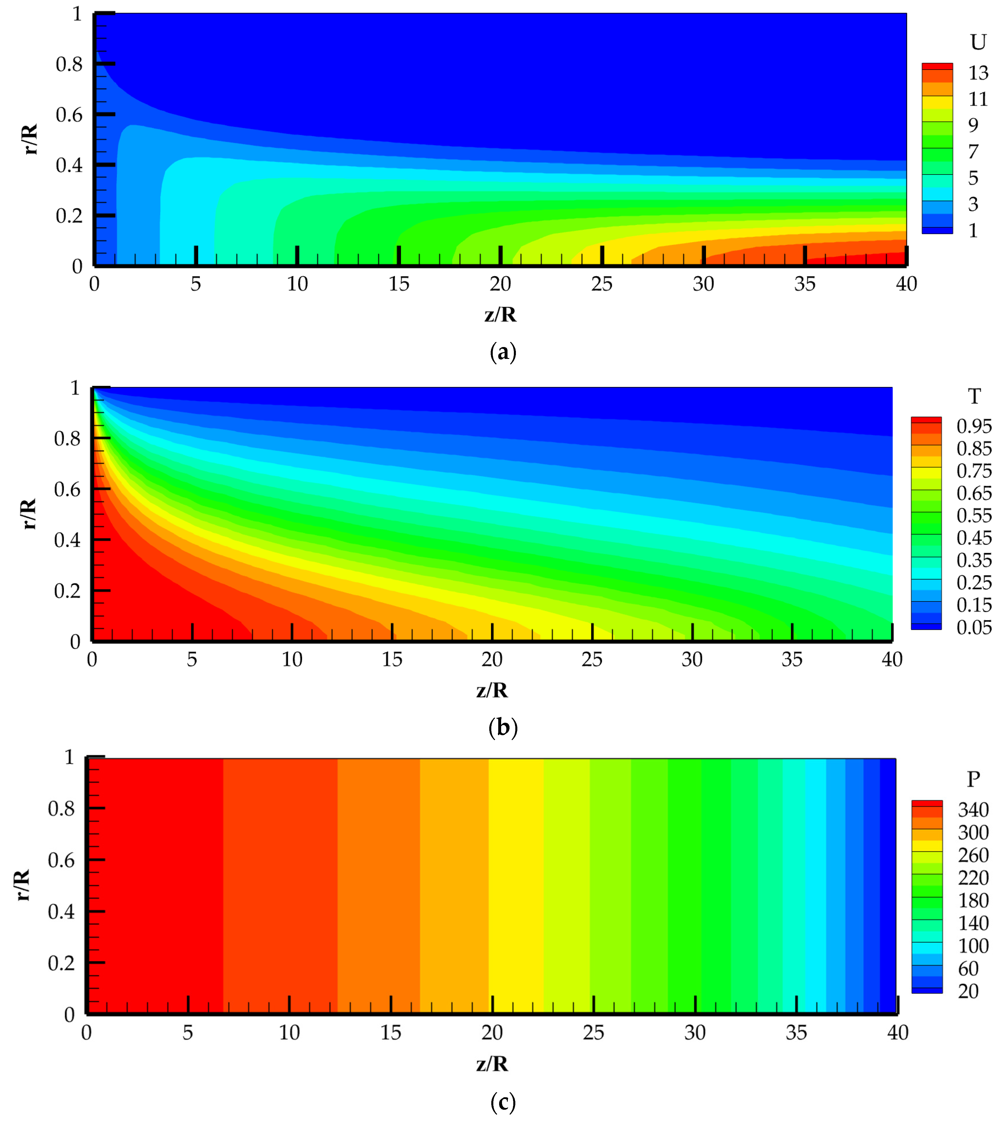
Contour plots of axial velocity U, excess temperature θ, and pressure P are shown in Figure 7. The maximum value of axial velocity U_m is found in the length interval z/R from 23 to 30 (see Figure 7a). In the central region, a core flow with maximum velocity U_m is visible. Subsequently, the contour plots of axial velocity U show a decrease in maximum velocity on the pipe axis. The contour of the stagnation zone, where the axial velocity is U = 0, increases in radius from the wall to a distance of r/R = 0.675. Further, the thickness of the stagnation zone begins to decrease along the pipe length (see Figure 7a). The contour plot of excess temperature θ shows a decrease in its magnitude along the pipe length (see Figure 7b). Cooling of the fluid causes a decrease in temperature, increase in plastic viscosity, and yield stress along the pipe radius. This accounts for the shape of the axial velocity profile U, featuring a consistent core within the axial zone. The contour plot of pressure P illustrates its constancy across the pipe cross-section with the maximum value at the initial sections of the pipe (see Figure 7c). The contour shows a decrease in pressure P for the pumping of paraffinic oil along the pipe length (see Figure 7c).

In Figure 8 and Figure 9, computational data for axial velocity U, excess temperature θ, and pressure P are presented at the operating parameters u₁ = 0.10 m/s; t₁ = 25 °C; t_w = 10 °C; Re = 523; Bn = 8.51; $\chi =$ 0.15.

In this regime, the Bingham number Bn = 8.51 is much smaller compared to the previous cases and expresses the viscoplastic state of the fluid. A weak occurrence of the viscoplastic state can be observed in the profiles of axial velocity U. The maximum velocity value decreases to U_m = 3.8 (see Figure 8a), and the stagnation zone is practically absent. The wall temperature of t_w = 10 °C leads to the equalization of the excess temperature profile θ along the pipe length (see Figure 8b). The pressure P distribution decreases almost linearly along the pipe length (see Figure 8c).

Contour plots of axial velocity U, excess temperature θ, and pressure P are presented in Figure 9. One can see a clear illustration of the change in the axial velocity profile of axial velocity U, excess temperature θ, and pressure P along the pipe length (see Figure 9).

Figure 10 and Figure 11 show calculated data of axial velocity U, excess temperature θ, and pressure P at regime parameters u₁ = 0.15 m/s; t₁ = 25 °C; t_w = 0 °C; Re = 785; Bn = 411.16; $\chi =0.15$.

As can be seen from Figure 10a, the profile of the axial velocity U at section z/R = 10 corresponds to the viscoplastic fluid flow with a core of constant velocity in the axial zone. The stagnation zone is from r/R = 0.62 to the pipe wall r/R = 1. Furthermore, the stagnation zone expands and occupies half of the pipe radius from r/R = 0.5 to r/R = 1. The maximum value of the axial velocity is U_m = 13.4 in the flow core along the pipe length from z/R = 35 to z/R = 40.

Increasing the flow velocity to u₁ = 0.15 m/s slows the rate of decrease of the excess temperature θ (see Figure 10b). The temperature remains sufficiently high, t = 10 °C, near the outlet boundary of the pipe at z/R = 39.90. The pressure distribution P decreases nonlinearly along the pipe length (see Figure 10c).

Contour plots of the axial velocity U, excess temperature θ, and pressure P clearly illustrate the variation of the sought parameters along the pipe length (see Figure 11).

Figure 12 and Figure 13 present the results of calculations for the axial velocity U, excess temperature θ, and pressure P at regime parameters of u = 0.10 m/s; t₁ = 25 °C; t_w = 0 °C; Re = 523; Bn = 411.16; $\chi =0.30$.

In this regime, the paraffin concentration is equal to $\chi =0.30$, which is two times higher than in the previous cases and increases the latent heat of phase transition. This affects the profiles of the axial velocity U, excess temperature θ, and pressure P (see Figure 12). An increase in the heat of phase transition leads to an increase in the axial velocity U. The maximum value of axial velocity U_m = 16 occurs along the pipe length from z/R = 29 to z/R = 40 (see Figure 12a). The value of the stagnation zone radius is r/R = 0.475 within the same pipe length interval. Profiles of the excess temperature θ also increase due to the increase in the heat of phase transition (see Figure 12b). Increasing the heat of phase transition reduces the plastic viscosity μ_P and the yield stress τ₀ of paraffinic oil, resulting in a decrease in the pressure value P along the pipe length (see Figure 12c).

The contour plots clearly illustrate the influence of increasing the heat of phase transition on the changes in profiles of axial velocity U, excess temperature θ, and pressure distribution P along the pipe length (see Figure 13).

Contour plots of the effective viscosity μ_eff/μ_P1 are presented in Figure 14 under the regime parameters of u₁ = 0.10 m/s; t₁ = 25 °C; t_w = 0 °C; Re = 523; Bn = 411.16; $\chi =$ 0.15 (a); $\chi =$0.30 (b).

When the concentration of paraffin is $\chi =$ 0.15, the distributions of effective viscosity μ_eff/μ_P1 are limited along the pipe length. The maximum value of effective viscosity occupies most of the pipe (see Figure 14a).

When paraffin concentration is equal to $\chi =$ 0.30, the value of latent heat of phase transition increases. Temperature also increases, and plastic viscosity and yield stress decrease. The distributions of effective viscosity μ_eff/μ_P1 are not limited along the pipe length, and the maximum value occupies the near-wall region (see Figure 14b).

5. Conclusions

A mathematical model of the non-isothermal laminar flow of paraffinic oil in a pipe by heat exchange with the environment has been developed and numerically simulated. The fluid’s Newtonian characteristics at the pipe’s outset gradually shift to the viscoplastic behavior typical of Shvedoff–Bingham fluid further along the pipeline.

The value of the axial velocity U in the near-axis zone increased significantly when the fluid moved along the pipe. In the near-wall region, on the contrary, the axial velocity U decreases, and the thickness of the region with zero velocity increases. This is due to the viscoplastic properties of the non-Newtonian fluid. The stagnation zone with zero velocity gradually increases as the non-Newtonian fluid (paraffinic oil) flows through the pipe.

The excess temperature decreases down the pipe length due to heat exchange with the surrounding environment, leading to the transition of paraffinic oil into a viscoplastic state. A significant increase in effective viscosity in the near-wall region of the pipe is demonstrated.

The pressure remains constant across the section and reaches its maximum value at the pipe inlet for pumping viscoplastic fluid. The pressure distribution becomes more nonlinear with an increasing Bingham number and decreases along the pipe length.

Thus, the novelty of the research lies in the transition of a Newtonian fluid into a viscoplastic state due to heat exchange with the environment. The obtained velocity, temperature, and pressure distribution profiles express the above transformation in the properties of non-isothermal laminar flow in a pipe.

One of the potential applications of the obtained results is the non-isothermal laminar flow of paraffinic oil in main oil pipelines, both underground and in subsea offshore fields.

References

- Zhapbasbayev, U.K.; Ramazanova, G.I.; Bossinov, D.Z.; Kenzhaliyev, B.K. Flow and heat exchange calculation of waxy oil in the industrial pipeline. Case Stud. Thermal Eng. 2021, 26, 101007. [Google Scholar] [CrossRef]
- Aiyejina, A.; Chakrabarti, D.P.; Pilgrim, A.; Sastry, M.K.S. Wax formation in oil-pipelines: A critical review. Int. J. Multiphase Flow 2011, 37, 671–694. [Google Scholar] [CrossRef]
- Chala, G.T.; Sulaiman, S.A.; Japper-Jaafar, A. Flow start-up and transportation of waxy crude oil in pipelines—A review. J. Non-Newton. Fluid Mech. 2018, 251, 69–87. [Google Scholar] [CrossRef]
- Ghannam, M.T.; Hasan, S.W.; Abu-Jdayil, B.; Esmail, N. Rheological properties of heavy & light crude oil mixtures for improving flow ability. J. Petrol. Sci. Eng. 2012, 81, 122–128. [Google Scholar] [CrossRef]
- Sanjay, M.; Simanta, B.; Kulwant, S. Paraffin problems in crude oil production and transportation: A review. SPE Prod. Facil. 1995, 10, 50–54. [Google Scholar] [CrossRef]
- Ribeiro, F.S.; Souza Mendes, P.R.; Braga, S.L. Obstruction of pipelines due to paraffin deposition during the flow of crude oils. Int. J. Heat Mass Transf. 1997, 40, 4319–4328. [Google Scholar] [CrossRef]
- Bekibayev, T.T.; Zhapbasbayev, U.K.; Ramazanova, G.I.; Minghat, A.D.; Bosinov, D.Z. Simulation of oil pipeline shutdown and restart modes. Compl. Use of Min. Resour. 2021, 316, 15–23. [Google Scholar] [CrossRef]
- Bostanjiyan, S.A.; Merzhanov, A.G.; Khudiev, S.I. On the hydrodynamic thermal “explosion”. Rep. Acad. Sci. USSR 1965, 163, 133–136. Available online: https://www.mathnet.ru/links/e54928daa8dbbddb9d34a0066504a779/dan31312.pdf (accessed on 4 February 2024). (In Russian).
- Bostanjiyan, S.A.; Chernyaeva, S.M. On the hydrodynamic thermal “explosion” of non-Newtonian fluid. Rep. Acad. Sci. USSR 1966, 170, 301–304. Available online: https://www.mathnet.ru/links/f8a68735fd8c01274d136d8dc40e7126/dan32553.pdf (accessed on 4 February 2024). (In Russian).
- Duvaut, G.; Lions, J.-L. Inequalities in Mechanics and Physics; Springer: Berlin, Germany, 1976. [Google Scholar] [CrossRef]
- Kim, J.U. On the initial-boundary value problem for a Bingham fluid in a three-dimensional domain. Trans. Am. Math. Soc. 1987, 304, 751–770. [Google Scholar] [CrossRef]
- Baranovskii, E.S. On flows of Bingham-type fluids with threshold slippage. Adv. Math. Phys. 2017, 2017, 7548328. [Google Scholar] [CrossRef]
- Vinay, G.; Wachs, A.; Agassant, J.-F. Numerical simulation of non-isothermal viscoplastic waxy crude oil flows. J. Non-Newton. Fluid Mech. 2005, 128, 144–162. [Google Scholar] [CrossRef]
- Min, T.; Choi, H.G.; Yoo, J.Y.; Choi, H. Laminar convective heat transfer of a Bingham plastic in a circular pipe II. Numerical approach hydrodynamically developing flow and simultaneously developing flow. Int. J. Heat Mass Transf. 1997, 41, 3689–3701. [Google Scholar] [CrossRef]
- Hammad, K.J. The effect of hydrodynamic conditions on heat transfer in a complex viscoplastic flow field. Int. J. Heat Mass Transf. 2000, 43, 945–962. [Google Scholar] [CrossRef]
- Moraga, N.O.; Andrade, M.; Vasco, D. Unsteady conjugate mixed convection phase change of a power law non-Newtonian fluid in a square cavity. Int. J. Heat Mass Transf. 2010, 73, 671–692. [Google Scholar] [CrossRef]
- Patel, S.A.; Chhabra, R.P. Heat transfer in Bingham plastic fluids from a heated elliptical cylinder. Int. J. Heat Mass Transf. 2014, 53, 3308–3318. [Google Scholar] [CrossRef]
- Danane, F.; Boudiaf, A.; Mahfoud, O.; Ouyahia, S.-E.; Labsi, N.; Benkahla, Y.K. Effect of backward facing step shape on 3D mixed convection of Bingham fluid. Int. J. Therm. Sci. 2020, 147, 106116. [Google Scholar] [CrossRef]
- Bird, R.B.; Curtiss, C.F.; Armstrong, R.C.; Hassager, O. Dynamics of Polymeric Liquids; Wiley: New York, NY, USA, 1987. [Google Scholar]
- Beverly, C.R.; Tanner, R.I. Numerical analysis of three-dimensional Bingham plastic flow. J. Non-Newton. Fluid Mech. 1992, 42, 85–115. [Google Scholar] [CrossRef]
- Schwedoff, T. Recherches expérimentales sur la cohésion des liquids. J. Phys. Theor. Appl. 1890, 9, 34–46. [Google Scholar] [CrossRef]
- Bingham, E.C. Fluidity and Plasticity; McGraw-Hill: New York, NY, USA, 1922. [Google Scholar]
- Barnes, H.A. The yield stress—A review or ‘παντα ρει’−everything flows? J. Non-Newton. Fluid Mech. 1999, 81, 133–178. [Google Scholar] [CrossRef]
- Klimov, D.M.; Petrov, A.G.; Georgievsky, D.V. Viscous-Plastic Flows: Dynamical Chaos, Stability, and Confusion; Nauka: Moscow, Russia, 2005. (In Russian) [Google Scholar]
- Papanastasiou, T.C. Flows of materials with yield. J. Rheol. 1987, 31, 385–404. [Google Scholar] [CrossRef]
- Voller, V.R.; Prakash, C. A fixed grid numerical modelling methodology for convection-diffusion mushy region phase-change problems. Int. J. Heat Mass Transf. 1987, 30, 1709–1719. [Google Scholar] [CrossRef]
- Henry, H.; Argyropoulos, S.A. Mathematical modelling of solidification and melting: A review. Model. Simul. Mater. Sci. Eng. 1996, 4, 371–396. [Google Scholar] [CrossRef]
- Patankar, S. Numerical Heat Transfer and Fluid Flow; CRC Press: Boca Raton, FL, USA, 1980. [Google Scholar] [CrossRef]
- Pakhomov, M.A.; Zhapbasbayev, U.K. RANS modeling of turbulent flow and heat transfer of non-Newtonian viscoplastic fluid in a pipe. Case Stud. Therm. Eng. 2021, 28, 101455. [Google Scholar] [CrossRef]
- Sahu, K.C. Linear instability in a miscible core-annular flow of a Newtonian and a Bingham fluid. J. Non-Newton. Fluid Mech. 2019, 264, 159–169. [Google Scholar] [CrossRef]
Figure 1.
Flow configuration scheme: 1—Newtonian fluid flow; 2—non-Newtonian fluid flow.
Figure 2.
Profiles of dimensionless axial velocity (a) and dynamic viscosity (b) across the pipe section. The points are the calculation data from [30]; lines are the authors’ calculation: Re = ρ1Ru1/μ1 = 1000; Sc = 10; Bn = 5; R1/R = 0.55; q/R = 0.1; μP/μ1 = 10; 1—Bn = 0; 2—Bn = 5.
Figure 3.
Radial profiles of dimensionless longitudinal velocity (a) and temperature (b) across the pipe section. The points are the calculation data from [14], lines are the authors’ calculation: 1 − Y = 0 (Newtonian fluid), 2 − Y = 1.99.
Figure 4.
Profiles of axial velocity U (a), temperature θ (b), and pressure distribution P (c) at the regime parameters: u1 = 0.10 m/s; t1 = 25 °C; tw = 0°C; Re = 523; Bn = 411.16; 0.15.
Figure 5.
Contour plots of axial velocity U (a), temperature θ (b), pressure P (c) at operating parameters u1 = 0.10 m/s; t1 = 25 °C; tw = 0 °C; Re = 523; Bn = 411.16; 0.15.
Figure 6.
Profiles of axial velocity U (a), temperature θ (b), and pressure P distribution (c) at the regime parameters: u1 = 0.10 m/s; t1 = 25 °C; tw = 5 °C; Re = 523; Bn = 59.14; 0.15.
Figure 7.
Contour plots of axial velocity U (a), temperature θ (b), pressure P (c) at operating parameters u1 = 0.10 m/s; t1 = 25 °C; tw = 5 °C; Re = 523; Bn = 50.14; 0.15.
Figure 8.
Profiles of axial velocity U (a), temperature θ (b), and pressure distribution P (c) at the regime parameters: u1 = 0.10 m/s; t1 = 25 °C; tw = 10 °C; Re = 523; Bn = 8.51; 0.15.
Figure 9.
Contour plots of axial velocity U (a), temperature θ (b), pressure P (c) at operating parameters u1 = 0.10 m/s; t1 = 25 °C; tw = 10 °C; Re = 523; Bn = 8.51; 0.15.
Figure 10.
Profiles of axial velocity U (a), temperature θ (b), and pressure distribution P (c) at the regime parameters u1 = 0.15 m/s; t1 = 25 °C; tw = 0 °C; Re = 785; Bn = 411.16; 0.15.
Figure 11.
Contour plots of axial velocity U (a), temperature θ (b), pressure P (c) at operating parameters u1 = 0.15 m/s; t1 = 25 °C; tw = 0 °C; Re = 785; Bn = 411.16; 0.15.
Figure 12.
Profiles of axial velocity U (a), temperature θ (b), and pressure distribution P (c) at the regime parameters u1 = 0.10 m/s; t1 = 25 °C; tW = 0 °C; Re = 523; Bn = 411.16; .
Figure 13.
Contour plots of axial velocity U (a), temperature θ (b), pressure P (c) at operating parameters u1 = 0.10 m/s; t1 = 25 °C; tw = 0 °C; Re = 523; Bn = 411.16; 0.30.
Figure 14.
Contour plots of effective viscosity at the following regime parameters: u1 = 0.10 m/s; t1 = 25 °C; tw = 0 °C; Re = 523; Bn = 411.16; 0.15 (a); 0.30 (b).