Review

A Review of Fusion and Tokamak Research Towards Steady-State Operation: A JAEA Contribution

Japan Atomic Energy Agency/ 311-0193, Naka Fusion Institute, Mukoyama 801-1, Naka-city, Ibaraki, Japan
Energies 2010, 3(11), 1741-1789; https://doi.org/10.3390/en3111741
Submission received: 30 September 2010 / Revised: 29 October 2010 / Accepted: 1 November 2010 / Published: 10 November 2010
(This article belongs to the Special Issue Nuclear Fusion)

Abstract

:
Providing a historical overview of 50 years of fusion research, a review of the fundamentals and concepts of fusion and research efforts towards the implementation of a steady state tokamak reactor is presented. In 1990, a steady-state tokamak reactor (SSTR) best utilizing the bootstrap current was developed. Since then, significant efforts have been made in major tokamaks, including JT-60U, exploring advanced regimes relevant to the steady state operation of tokamaks. In this paper, the fundamentals of fusion and plasma confinement, and the concepts and research on current drive and MHD stability of advanced tokamaks towards realization of a steady-state tokamak reactor are reviewed, with an emphasis on the contributions of the JAEA. Finally, a view of fusion energy utilization in the 21st century is introduced.

1. Introduction

Fusion research to provide a scientific basis for fusion energy production has been carried out for 50 years [1]. World fusion research is ultimately directed to the construction and demonstration of a fusion power station in DEMO and to play a meaningful role in the energy supply at the end of this century [2,3]. Fusion research is a combination of: (1) the development of a scientific basis for plasma confinement and enabling technologies for fusion; (2) demonstrations of fusion-relevant plasma cores and technologies for fusion energy and (3) the integrated demonstration of fusion power production. The continued interaction among these three areas of research is fundamental to the success of fusion research.
To achieve such a goal, a fundamental understanding of fusion and plasma confinement is essential [3]. Over the past 50 years of fusion research, significant progress has been made in the area of (1) and we have reached the stage of the demonstration of the scientific and technological feasibility of fusion energy by ITER [4]. Research area (1) can be developed independently if the issues are clearly understood.
The development of (2) requires an integrated understanding of the system concept since the system imposes many constraints and interlinkages among the various physics. This leads to the need for the development of the reactor concept. In 1990, we developed a steady-state tokamak (from the transliteration of the Russian sentence toroidal'naya kamera s aksial'nym magnitnym polem or toroidal chamber with an axial magnetic field) reactor concept called SSTR best utilizing the bootstrap current [5] and its conceptual design [6,7]. The conceptual development of the SSTR (Steady State Tokamak Reactor) was done for this purpose and to implement this philosophy into large tokamak experiments [8]. Since then, significant efforts to achieve reactors relevant high temperature plasma and provide a scientific basis for ITER and the SSTR have been made in JT-60 and JT-60U during 23 years of research operation exploring advanced regimes relevant to the steady state operation of tokamaks. The progress and findings in these areas are presented in a topical review of Nuclear Fusion [8], a special issue of Fusion Science and Technology [9], IAEA conferences [10,11,12,13,14,15,16,17,18,19,20,21], American Physical Society meetings [22,23,24,25,26,27,28,29,30,31,32,33,34,35,36,37,38,39], European Physical Society meetings [40,41,42,43,44,45,46,47,48,49,50,51,52,53,54], and the AIP conference series (IMFP2009) [55].
This paper starts from a review of fusion energy and the principles of magnetic confinement in Section 2, followed by the principles of the steady state tokamak reactor in Section 3, parallel collisional transport physics for the operation of a steady state tokamak in Section 4, MHD stability of the advanced tokamak in Section 5, the role of fusion energy in the 21st century in Section 6 and Summary and Acknowledgements in Section 7.

2. Fusion Energy and Magnetic Confinement
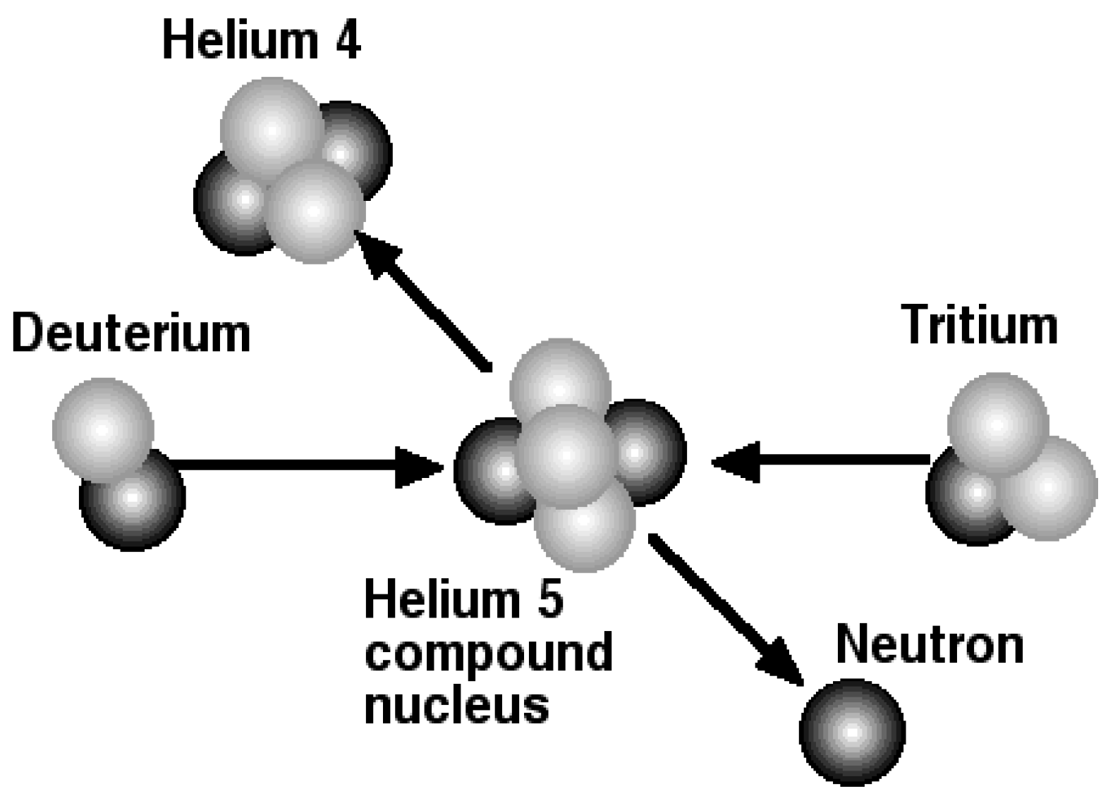
2.1. Fusion Energy

The question of energy development using fusion reactions appeared in the early 20th century when the theory of relativity and quantum mechanics was proposed. German physicist W. Heisenberg (1901–1976), who initiated quantum mechanics in early 20th century, recorded discussions with Danish physicist Niels Bohr (1885–1962) and Lord Rutherford (1871–1937) in Chapter 13—Atomic Power and Elementary Particles (1935–1937) of his book “Physics and Beyond”. In 1942, the inventor of the fission reactor, Italian physicist Enrico Fermi (1901–1954), while having a lunch at the Columbia Faculty Club, suggested to Edward Teller (1908–2003) the possibility of burning deuterium to develop a large source of energy. Based on his suggestion, Teller made various calculations and found that fusion between deuterium (D) and tritium (T) is a possibility. Tritium and deuterium react at relatively low energy, creating Helium and a neutron. Since helium has a higher binding energy, we can generate a huge amount of energy.
The deuterium nucleus consists of one proton and one neutron. Among combinations of the two nuclei, p-p, n-n and p-n, a bound state is only possible for p-n, which is deuterium. Deuterium was discovered in 1932 by American chemist H.C. Urey (1893–1981, 1934 Nobel Prize for Chemistry), who showed that one out of 7,000 hydrogen atoms is deuterium. The bound state of a proton and a neutron to form deuterium can be treated as a two-body problem of nuclear force between neutron and proton originated from the meson exchange forces, as predicted by Japanese Nobel Prize Winner Hideki Yukawa (1907–1981). He explained this strong force as an exchange force of a finite mass meson to get short-range force in marked difference with Coulomb force explained by the mass-less photon exchange force. The wave function inside the box type nuclear potential may be approximated by a sine function AsinK(r-c) (A and K are constants, c is minimum distance). The wave function outside the nuclear potential may be Be−kr (B, k are constants). Decay rate k of the wave function is related with the binding energy as k~Eb0.5, which implies that radial decay o the wave function is weak and two-nucleon probability stays outside of nuclear potential, which becomes larger (~/ru/2~e−2kr from Born relation) if Eb is small. In other words, the two nucleons are not strongly bonded and are easy to separate. Conversely, if the binding energy Eb is large, the wave function decays rapidly outside the nuclear potential, leaving the separation probability of nucleons as small. The binding energy of deuterium (Eb = 2.225MeV) is small and the wave function decays slowly in the r direction. The small binding energy of deuterium resulted in the dissociation of deuterium into a proton and a neutron at the high radiation temperature of the early Universe, by which formation of Helium is delayed to three minutes after the Big Bang and the reason we have so much hydrogen remaining in the Universe.
Hydrogen with mass number 3 is called tritium. The word “tritium” comes from the Greek word meaning “third”. The nucleus of tritium consists of one proton and two neutrons. Tritium is an unstable isotope and decays into helium-3 by emitting a high-energy electron and a neutrino (T→3He + e + ν). This is called beta decay and has a half-life of 12.26 years. Tritium was first produced in the laboratory by Australian physicist M. Oliphant (1901–2000) in 1934 by colliding deuterium.
Tritium as a fuel for DT fusion is generated by the nuclear reaction of neutrons with lithium. Lithium has two isotopes (6Li and 7Li) and the abundance of 6Li and 7Li in natural Li is 7.4% and 92.4%, respectively. The 6Li reaction 6Li + n→3T + 4He + 4.8MeV is an exothermic reaction, while the 7Li reaction 7Li + n→3T + 4He + n'−2.5MeV is an endothermic reaction. The cross section of the 6Li reaction is of 1/v type and easy to react at low energy. Meanwhile, the 7Li reaction is called a threshold reaction whose cross section becomes nonzero above a critical energy. The reaction rate for 6Li is much larger than that for 7Li. The amount of lithium in seawater is about 233 billion tons and it can be considered an infinite resource if low-cost technologies for the recovery of lithium from seawater were established.
Neutrons were discovered by the British physicist J. Chadwick (1891–1974) in 1932. Neutrons have no net charge, but in the center there is slightly positive charge distribution, which is cancelled by a slightly negative charge distribution in the periphery. The mass is distributed within a radius of about 0.8 fermi. The neutron is slightly heavier than the proton and the difference is about twice the electron mass (1.29MeV). Neutrons alone can’t exist stably, and decay to a proton emitting the electron and a neutrino with a half-life of about 12 minutes (n→p + e + ν). The mass of the neutron is greater than the sum of the mass of a proton and an electron, and the mass difference leads to the energy release. This reaction was confirmed in 1948 by the observation of the electrical bending of protons and electrons from the beta decay of a strong neutron beam in a large cylindrical tank. Natural decay of isolated particles always seems to end with a decrease in mass. Since the mass of a neutron is larger than that of proton by about two times the electron mass, a neutron easily decays to a proton while it is difficult for a proton to decay to a neutron. Indeed, the question of whether proton decay occurs has been an important research subject in physics for many years.
Helium is an element with two protons and two neutrons and its mass number is four. The origin of the name of helium is Greek word “helios” meaning the Sun. During a solar eclipse observed in India on August 18 in 1868, British astronomer J.N. Lockyer (1836–1920), who launched the prominent scientific journal Nature, observed the solar corona and discovered a new emission spectrum. He thought that the emission came from an unknown element, which he called as “helium”. The binding energy of 4He is extremely large compared with those of hydrogen and lithium. Such a large binding energy for this particular nucleus is explained by the nuclear “shell model”.
The potential shape for a neutron is different from that of a proton since only the nuclear potential operates on neutrons while the Coulomb potential is superimposed for protons. In Helium, two nucleons with + 1/2 and −1/2 spins can sit in the ground state for a neutron and proton independently. 4He is the first element in the closed-shell state and “2” is the smallest “magic number”. This leads to the large binding energy of 4He. Thus, the 4He nucleus is particularly stable, and abundant in the Universe created by the Big Bang.
The encounter of deuterium and tritium results in the formation of the “compound nucleus” 5He ( D + T H e * 2 5 H 2 4 e + n ), as shown in Figure 1, by the tunnel effect at a fractional energy of 500 keV Coulomb barrier potential. The compound nucleus has a high reaction probability near 80 keV due to the resonance phenomenon. In this way, Nature gives human beings a chance to use this reaction for practical purposes. Strong nuclear force can operate beyond the Coulomb barrier when the distance r is less than 3 fermi if we use the nuclear radius formula Rc = 1.1A1/3 fermi (1fermi = 10−15m). The kinetic energy of the incident nuclei is distributed to the nuclei in the compound nucleus.
Figure 1. Schematic diagram of the DT fusion reaction via a compound nucleus. Encounter of deuterium and tritium produces 5He compound nucleus and emits a 3.52 MeV 4He and a 14.06 MeV neutron.
Energies 03 01741 g001
A neutron and helium that achieve a large energy by chance will escape from the compound nucleus. Fusion cross section considering tunnel effect and resonance is given as:
σ r = π D 2 P ( E / E c ) Γ i Γ f ( E E r ) 2 + Γ 2 / 4
where, ƛ2 = ћ2(2ME)−1 is de Broglie wave length/2π of incident nuclei. P(E/Ec) is a Coulomb barrier penetration probability, and the last factor is the Breit-Wigner nuclear resonance cross section. An analytical form of the Coulomb barrier penetration probability was given by Gamov as P(E/Ec) = (Ec/E)1/2exp(-(Ec/E)1/2), where Ec = mre4/8ε02ћ2 assuming E << Ec, where mr is the reduced mass (mamb/(ma + mb), e0 is the vacuum permittivity, and ћ is Planck's constant, respectively. The exact analytical form of the Coulomb barrier penetration probability, which is valid for arbitrary E/Ec, was given by N. F. Mott and H.S.W. Massey [56] as follows:
P ( E / E c ) = E c / E exp E c / E 1
The point for the derivation of above formula is the long-range nature of the Coulomb force. According to conventional wisdom, we assume the plane wave solution exp[ikz] as a boundary condition of the incident wave at infinity. Due to the long-range nature of Coulomb force, the incident wave is distorted even at infinity. The wave front should be perpendicular to the classical hyperbolic orbit and the incident wave is modified as exp[ik{z + b0lnk(r − z)}], where b0 = eiej/(4πε0mru2)=7.2 × 10−10ZiZj/Er(eV), where (m) is the Landau parameter. In fact, as seen in Figure 2, the measured fusion cross-section is fitted well by the truncated summation of equation (1) as σ r = σ 0 P ( E L / E c L ) [ { 1 + 4 ( E L E r L ) 2 / Γ L 2 } 1 + α ] [57].
Figure 2. DT Fusion cross section as a function of deuterium energy in laboratory frame EL, here σ0 = 23.6 b, EcL = 2.11 MeV, ErL = 78.65 keV, ΓL = 146 keV, α = 0.0081 and b is barn (10−28 m2).
Energies 03 01741 g002
A recent paper [58] revisited this fusion reaction questioning the discussion above and gave a simpler three-parameter fitting based on the approximate analytical collision cross section using the optical potential (= Ur + iUi) for D + T reaction. This simpler formula gives better agreement with the fusion cross-section data at low energy.

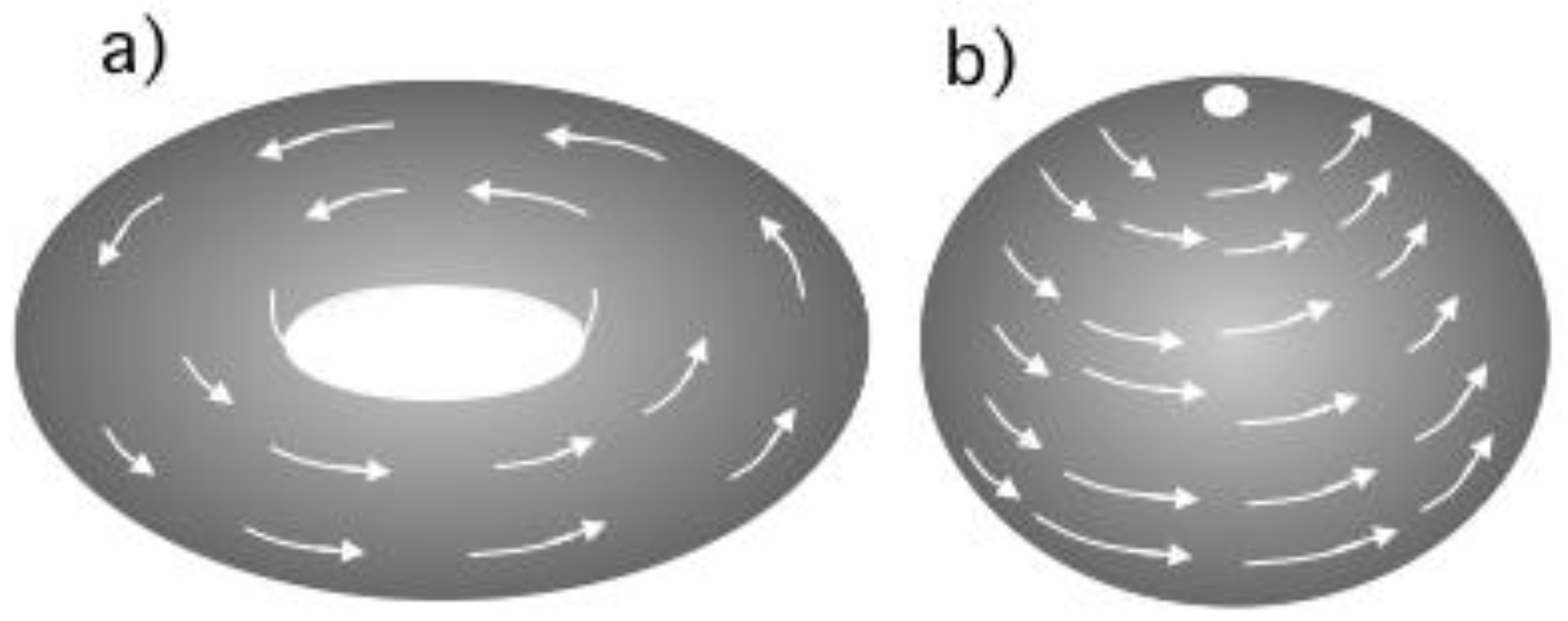
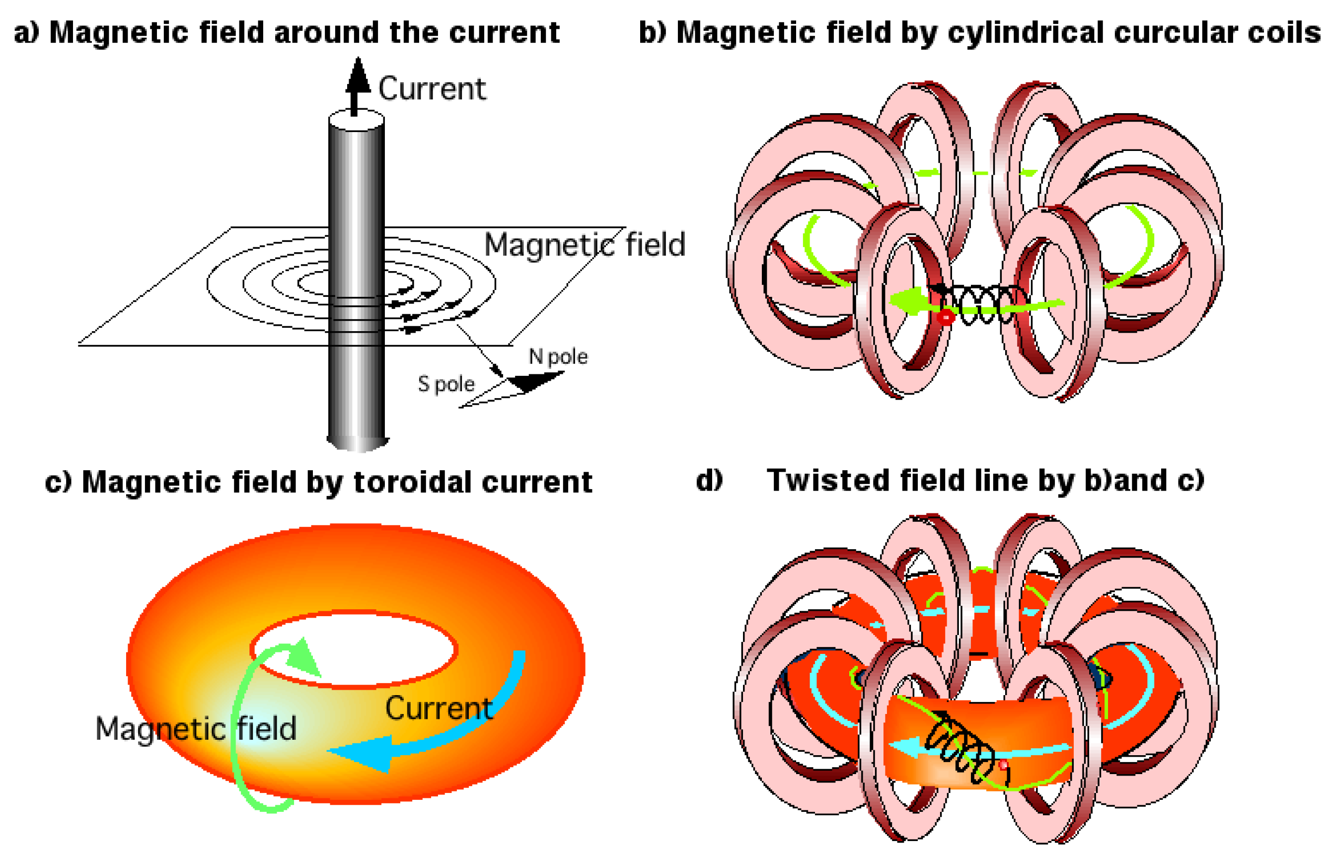
2.2. Topology and Symmetry of Magnetic Confinement Geometry

2.2.1. Topology

In the natural fusion reactor, the Sun, a dense and hot plasma, is confined with a gravitational field. The characteristic of this force is that it is a central force field and the force acts in the direction of the field lines. For this reason, the confinement bottle has a “Sphere” topology. In the man-made fusion reactor, a high temperature plasma is confined by trapping charged particles with the Lorentz force in a magnetic field to sustain the reaction within a small dimension a 100 millionth that of the Sun. The characteristic of this force is that it acts in the direction perpendicular to the field line. For this reason, the confinement bottle has a “torus” topology. In the MHD framework, plasma equilibrium is governed by a balance between the pressure gradient force and the Lorentz force. This requires “symmetry” for the field line structure. The tokamak configuration has symmetry in a toroidal direction, while “hidden” symmetry is required for a helical configuration.
Considering the magnetic confinement of a hot plasma in a region of three-dimensional space, the boundary must be a closed surface. The sphere is a typical closed surface but it can’t be covered with a non-zero vector field and it is always associated with a fixed point (or null point). In the torus, however, the surface can be covered with a non-zero vector field. In our case, we consider the magnetic field as a vector field. Mathematically speaking, all surfaces homeomorphic to a sphere will have a fixed point. This means that a sphere and a torus have different topologies. This surface property of a sphere and a torus shown in Figure 3 does not change, even if they are bent or stretched. A geometrical property, which does not change by continuous deformations, is called “topology”.
Figure 3. Characteristics of the vector fields in a torus and a sphere. It is possible to cover the torus with a non-zero vector field, but it is impossible to cover a sphere with a non-zero vector field (Brouwer’s fixed point theorem).
Energies 03 01741 g003
French mathematician Henri Poincare (1854–1912) proved the theorem “A closed surface that can be covered with a vector field without a fixed point is restricted to a torus.” This is called the “Poincare theorem” [59]. The meaning of Poincare theorem is important for high temperature plasma confinement. Considering the boundary surface of the magnetic confinement, the plasma will leak from the zero point of a magnetic field vector. To confine the hot plasma, the surface must be covered by non-zero magnetic field. This is why we use toroidal geometry for magnetic confinement.

2.2.2. Integrability and Symmetry in Plasma Equilibrium

The magnetic field is characterized by its incompressibility (∇ · B = 0). This leads to the existence of a vector potential A(∇ × A = B) given by A = φ∇θ − ψ∇ζ + ∇G (θ and ζ are arbitrary poloidal and toroidal angles, G is gauge transformation part). This leads to the Hamilton structure for the magnetic field evolution in the direction of toroidal angle ζ. The magnetic field line trajectory is given by dθ/dζ = ∂ψ/∂φ, dφ/dζ = −∂ψ/∂θ and can be regarded as the Hamilton equation if we regard ψ as the Hamiltonian, θ as the canonical coordinate, f as the canonical angular momentum, ζ as time. Variational principle of a field line is given by the analogy to the Hamilton action integral, S = ∫Ldt = ∫[p∇dq/dt − H]dt by substituting the relationship p→φ, q→θ, H→ψ, t→ζ as S=∫[φdθ/dζ − ψ]dζ =∫[φ∇θ − ψ∇ζ]·dx = ∫dx, so variational principle to give a field line is given by the following formula:
δ A d x = 0
In plasma equilibrium, the plasma's expansion force (−P) is balanced with the Lorentz force (J × B). Here, J is the current flowing in the plasma, B is the magnetic field, P is the plasma pressure. This is the basic principle of the magnetic confinement fusion:
J × B = P
In this case, the magnetic field lies on the constant pressure surface (B·∇P), called “integrable” and the surface is called the “magnetic surface”. This means that B is a linear combination of tangent vectors ∂x/∂θ and ∂x/∂ζ on the flux surface. The incompressibility condition of B leads to the existence of the flow function and the coordinate transformation of θ (θ°θm) by which B becomes a straight line gives the Clebsch form for the magnetic field B = ∇φ × ∇α, where α = θm−ζ/q. Then, φ and ψ becomes 1/2π of toroidal and poloidal fluxes inside the constant P surface and P=P(φ). The coordinates (φ, θm, ζ) are called flux coordinates. The Lagrangian of the magnetic field line L = φdθ/dζ − ψ becomes L = φdθm/dζ − ψ(φ). Therefore, the Lagrangian has no explicit dependence on “canonical coordinate” θm nor “time” ζ and they (θm and ζ) are ignorable coordinates. The action integral of a field line in flux coordinates is given by:
S = A d x = [ φ d θ m ψ d ζ ]
The existence of such ignorable coordinates is essential for the existence of plasma equilibrium. If there is apparent geometrical symmetry such as axisymmetry in a tokamak, it is easy to show the existence of a flux function. But, hidden symmetry can be found in general 3D toroidal geometry, called 3D equilibrium. For general 3D equilibrium, the action integral S is given by [60] as follows:
S = [ B 2 / 2 μ 0 + P / ( γ 1 ) ] d V
The equivalence of variational principle δS = 0 to equilibrium equation (4) is apparent from the following equation as shown by [60]:
δ S = ξ [ μ 0 1 ( × B ) × B P ] d V
This variational principle is implemented as numerical VMEC code for general toroidal equilibrium [61]. Plasma equilibrium with apparent symmetry in a torus is the axisymmetric magnetic configuration such as the tokamak configuration shown in Figure 4, which is a major object of present fusion research. In the cylindrical coordinate system (R, ζ, Z), the ζ is a cyclic coordinate and ∂/∂ζ = 0. Hamiltonian (or poloidal flux/2π) ψ is given by using the ζ component of the vector potential A as ψ = RAζ(R, Z).
The variational principle of plasma equilibrium in axisymmetric geometry is given by δS=0, where S = d R d Z = R ( B p 2 / 2 μ 0 B ζ 2 / 2 μ 0 P ) d R d Z [62]. The Euler-Lagrange equation for ψ is given by / ψ ( / ψ R ) / R ( / ψ Z ) / Z = 0 , which gives the following Grad-Shafranov equation [63,64]:
[ R / R ( R 1 / R ) + 2 / R 2 ] ψ = μ 0 R 2 P ( ψ ) + F F ( ψ )
This equation is simply the ζ component of ∇2A = −μ0J and can be solved numerically by giving functional form for P and F, which are determined by the transport processes. This plasma current becomes one of free energy sources in addition to plasma pressure to drive various MHD instabilities, which are described in Section 5.
Figure 4. How to create a tokamak configuration: (a) If the current flows, a magnetic field is generated around the current. (b) Arranging circular coils around the torus and energizing the coil produces a magnetic field in the toroidal direction. (c) Toroidal plasma current produces a magnetic field linking the torus. (d) Combination of (b) and (c) creates twisted magnetic field lines and is called a tokamak.
Energies 03 01741 g004

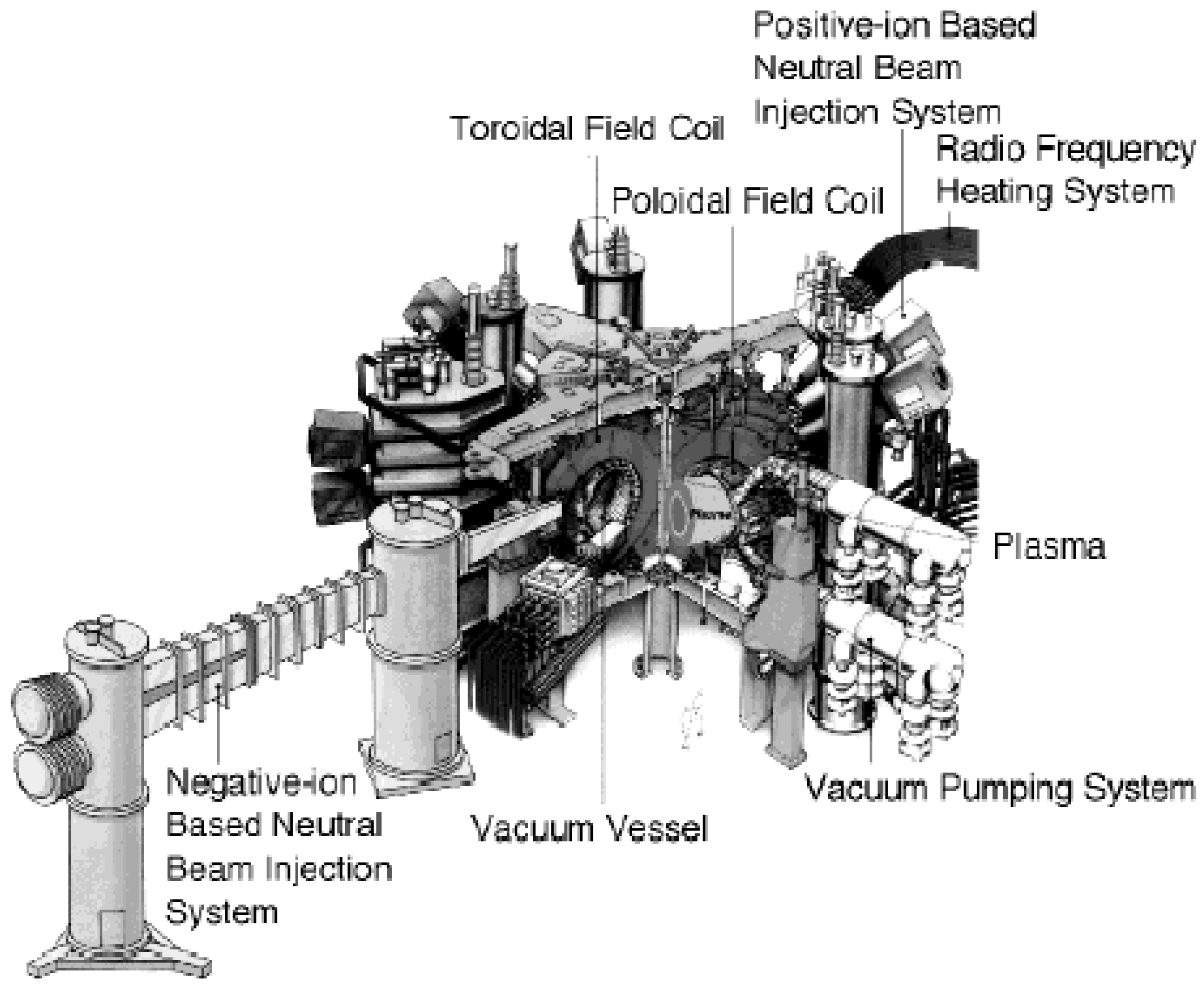
2.3. Tokamak as a Fusion Energy System

2.3.1. Tokamak Confinement and Inductive Operation

Tokamak has geometrical symmetry in the toroidal direction and this symmetry provides robustness in maintaining a nested flux surface against various parametrical changes leading this configuration to be a front-runner in fusion research. Tokamak achieved equivalent break-even conditions in large tokamaks such as JT-60U [8] and JET or produced significant fusion power (>10 MW) in TFTR [65] and JET [66], while other magnetic confinement fusion experiments remained much lower, as shown in Figure 5. Geometrical symmetry provides good confinement of energetic charged particles as well as thermal plasmas. This is a reason why the tokamak concept was selected for ITER.
However, this configuration requires a net toroidal plasma current [the right hand side of (8) is proportional to toroidal plasma current], which is driven mainly by inductive means. This method is quite effective since the electrical conductivity of 10 keV plasma is 20 times higher than that of Cu at room temperature. But induction of toroidal electric field is limited to a finite pulse length (300–500 seconds in ITER) due to current limits in the transformer (the CS coil current in ITER). This means that a tokamak fusion power station may be pulsed as shown in Figure 6 or it requires huge energy reservoir. The tokamak reactor design based on inductive operation was first made in UWMAK studies by R. Conn [67].
Figure 5. Lawson diagram (Ti(0), ni(0)τE). Tokamak confinement showed significant progresses by decades (1970s, 1980s, 1990s) to reach break-even conditions. The key is to achieve good confinement with collisionless high temperature plasmas.
Energies 03 01741 g005
Figure 6. Schematic view of the inductive operation of a tokamak. Change in the primary current induces a toroidal electric field to drive and sustain the plasma current.
Energies 03 01741 g006

2.3.2. Tokamak Continuous Operation

Since present power sources such as oil/coal/natural gas fired plants and fission plants operate continuously, it is highly desirable for a tokamak reactor to be a steady-state power station. To achieve continuous operation in a tokamak, a non-inductive current drive is essential. After the theoretical development of a current drive using lower hybrid waves by N.J. Fisch [68] and subsequent experimental demonstration in the JFT-2 [6], the STARFIRE design [70] was made to realize continuous fusion power production, which in turn showed that recirculation power is larger than expected.
Nature blesses human being by providing an interesting physical process, called “bootstrap current” to make tokamaks operate in steady-state [71,72]. The bootstrap current is driven by the collisional relaxation of a distorted velocity distribution function in a rare collision regime (called collisionless plasma), which is a kind of thermo EMF that drives the plasma current in a toroidal direction and 80% of the plasma current is thus driven by the bootstrap current, as shown in Figure 7 [73]. The physics of non-inductive current drive are governed by the collisional transport along the magnetic field. Since the power required for current drive reduces the net electricity from a fusion power station, efficient and also reliable non-inductive current drive methods have to be developed for steady state tokamak fusion plants, as described in Section 4.
Figure 7. Comparison of the experimental and theoretical bootstrap current fractions in JT-60 [73].
Energies 03 01741 g007

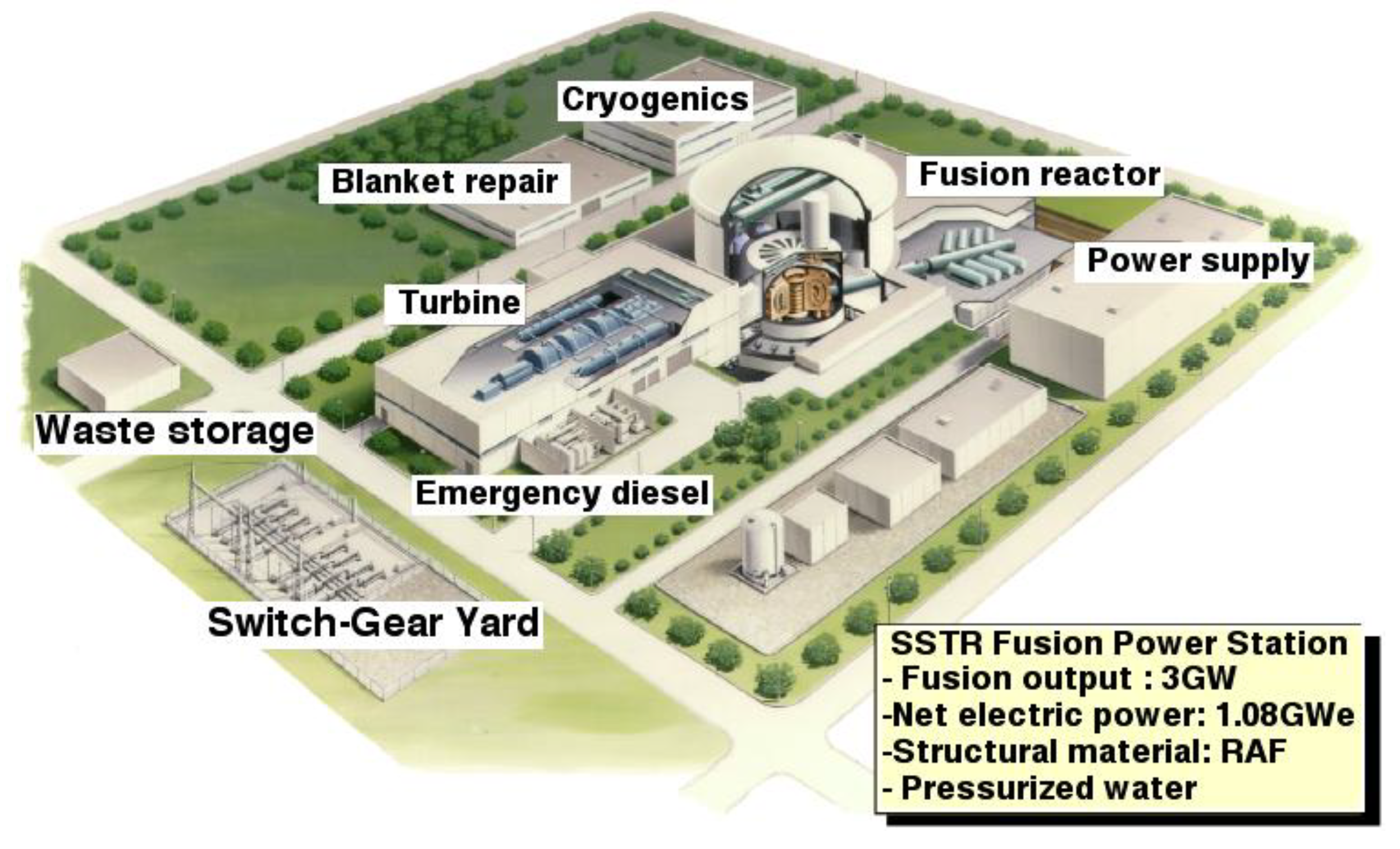
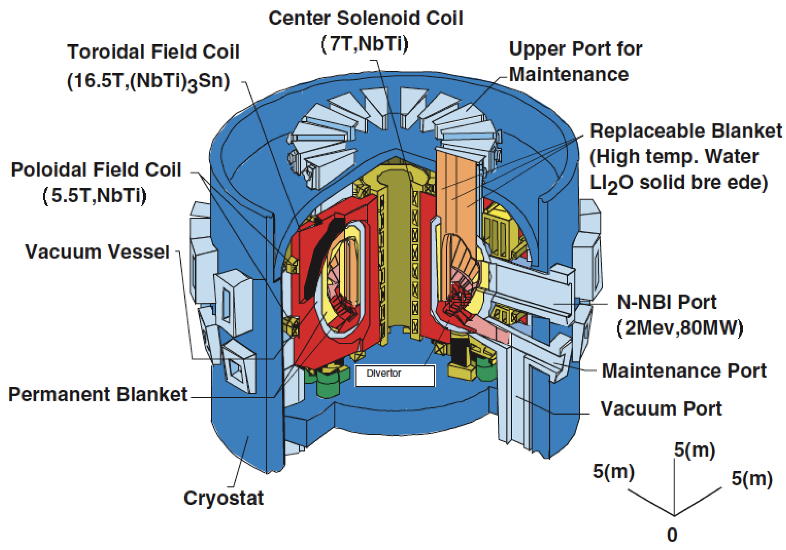
2.3.3. The Steady State Tokamak Reactor

Observation of a high bootstrap current fraction, up to 80% in the JT-60 high-βp discharges [73] stimulated the design development of a SSTR, consistent with updated scientific and technological knowledge at that time [5].
Figure 8. Bird’s eye view of SSTR(Steady State Tokamak Reactor) plant layout [7].
Energies 03 01741 g008
The SSTR concept was originally developed in 1989 as a DEMO concept (aiming to demonstrate sustained electric power generation from fusion) with minimum extrapolation from the knowledge in those days [5,6]. A power reactor concept with similar core plasma assumptions but more aggressive technical provisions, ARIES-I [74], was developed independently. Since then various concepts of a tokamak fusion power system have been developed on the basis of advanced tokamak scenarios with high bootstrap current and high confinement performance; namely A-SSTR [75], ARIES-RS [76], CREST [77]. The SSTR design was made with strong involvement of industries [78]. The plant layout is shown in Figure 8 and a bird’s eye view of the tokamak core is shown in Figure 9 [79].
Figure 9. Bird’s eye view of SSTR(Steady State Tokamak Reactor) tokamak core [79].
Energies 03 01741 g009

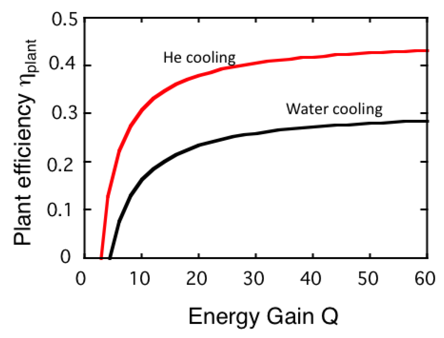
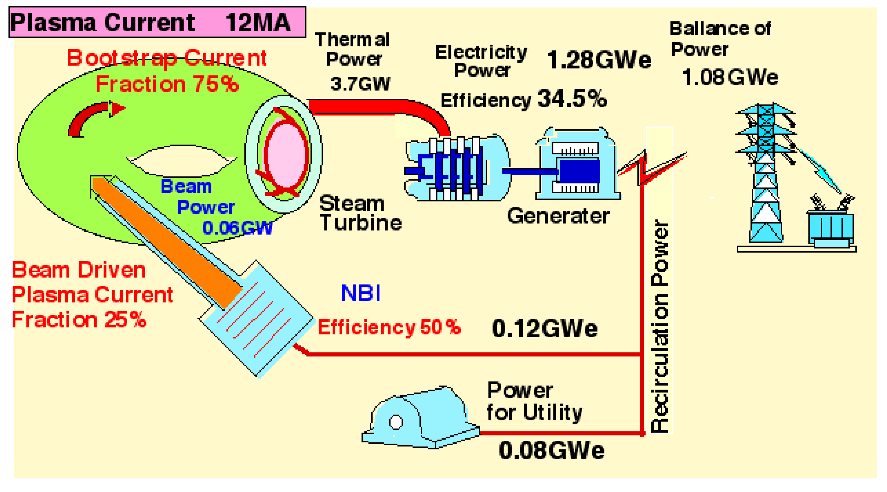
2.3.4. Reactor Power Balance

The SSTR concept as well as ARIES-I have provided good scientific and technical guidelines for fusion research and development in the World. Reactor power balance is an important aspect in SSTR [80]. The energy flow diagram of SSTR is shown in Figure 10. Here, Pf is the plasma fusion power, PCD is the current drive power, Q is the energy gain of the confined plasma Q = Pf/PCD, γBD is the energy multiplication factor in the blanket-divertor system, PGe is the gross electric power, PNet is the net electric power to the grid, rPGe is the re-circulating power (r is the re-circulating power fraction), γCD is the overall system efficiency of the CD system, and ηauxPth is the power required for auxiliary equipment.
Figure 10. Power flow diagram of SSTR [80].
Energies 03 01741 g010
From the relations in Figure 10, the plant efficiency ηPlant (=PNet/Pth), the ratio of net electric power output to thermal power output, is given by:
η p l a n t = η t h η a u x 1 γ C D γ B D ( 1 + Q )
Here, the thermal conversion efficiency ηth is 0.345 for water cooling in a fission light water reactor, while it is 0.49 for an advanced high temperature He cooling system. The second term of rhs is the reduction of plant efficiency due to auxiliary equipment, which ranges from 0.02–0.04. Power for auxiliary systems in SSTR is assumed to be 80 MW, similar to the STARFIRE design but an accurate evaluation is require,d based on ITER experience. The third term of rhs is specific for a tokamak power system and represents the current drive and heating requirements. The system efficiency of N-NBI is estimated to be 0.50, which is much higher than that of the laser driver in ICF, but the electric power of 120 MW is not small and represents one of drawbacks of helical system, that still requires basic research to improve plasma confinement at a reactor-relevant high temperature. The energy multiplication factor in a Blanket-divertor system γBD has to be evaluated considering various processes in the blanket and divertor. The nominal γBD value for SSTR is 1.21 (= 3710 MW/3060 MW) [78]. The ηplant-Q diagram is shown in Figure 11 for a pressurized-water cooling and a high temperature helium gas cooling system. It must be noted that ηplant depends weakly on Q at Q = 30 to 50, ηplant~0.3 for pressurized water and ηplant~0.4 for high temperature helium.
Figure 11. Plant efficiency ηplant as a function of energy gain Q for high temperature Helium cooling (ηth = 0.49) and water-cooling (ηth = 0.345). Parameters are chosen as ηaux = 0.03, γCD = 0.5, γBD = 1.21.
Energies 03 01741 g011
Efficiency of the current drive by non-inductive means (NBCD or RFCD) is expressed by the current drive efficiency ηCD, defined by ηCD = IpCDRp < ne >/PCD and has a certain limit ηCD~5 × 10¹⁹A/Wm2 which is much less than the efficiency of an inductive current drive. In this sense, it is difficult to achieve the required Q level of Q = 30 to 50 by only using non-inductive current drive by external means. This is a fundamental reason why we have to utilize the bootstrap current to achieve the efficient steady state operation of a tokamak reactor. Operation at some Q has two meanings since the CD system has two functions, current drive and heating. The first one is that current drive efficiency must be compatible with this Q value, to support the plasma current Ip with this current drive power. The second one is that the energy confinement time of the plasma must be compatible with this Q value.

3. Principle of a Steady State Tokamak Reactor

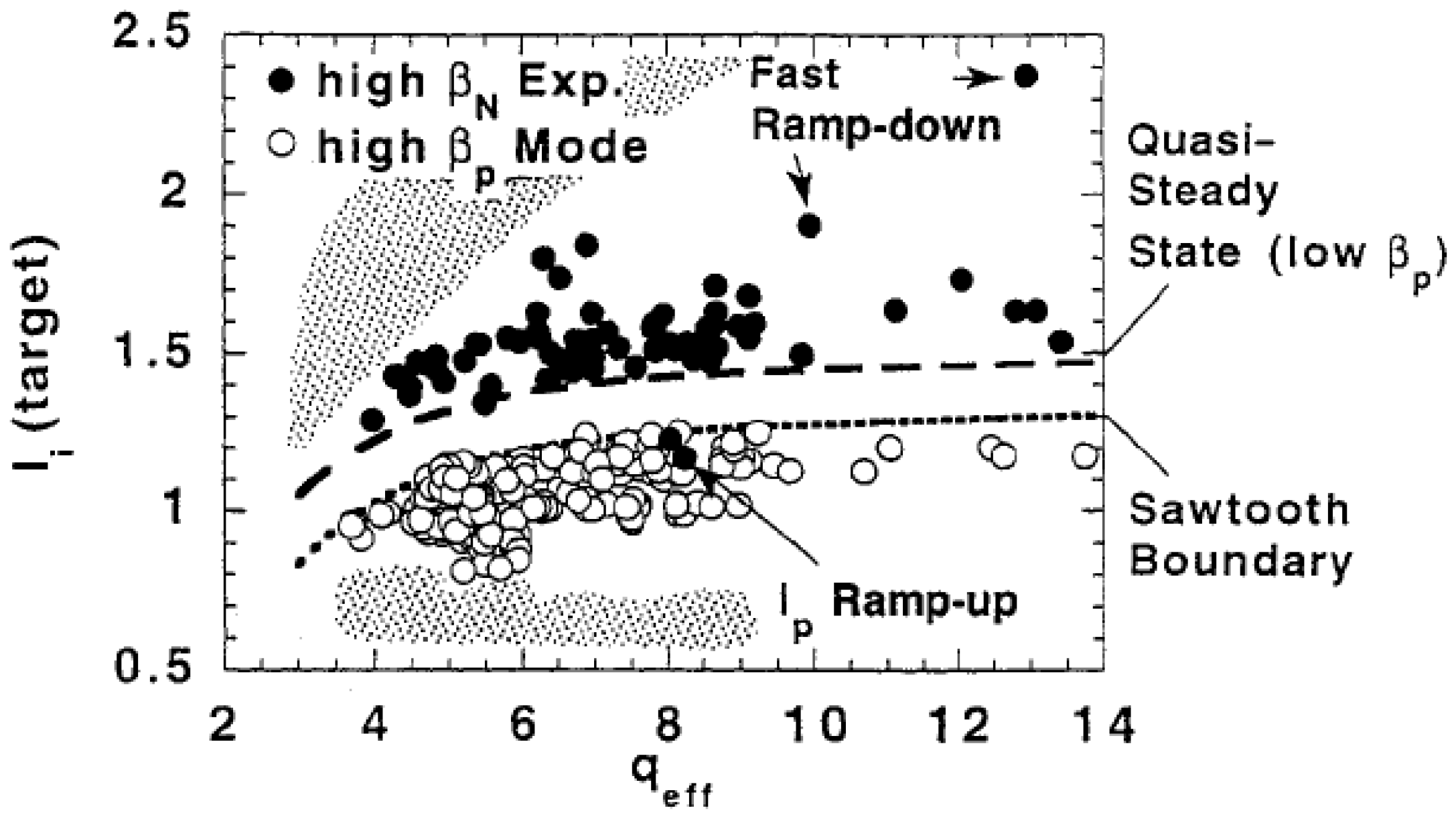
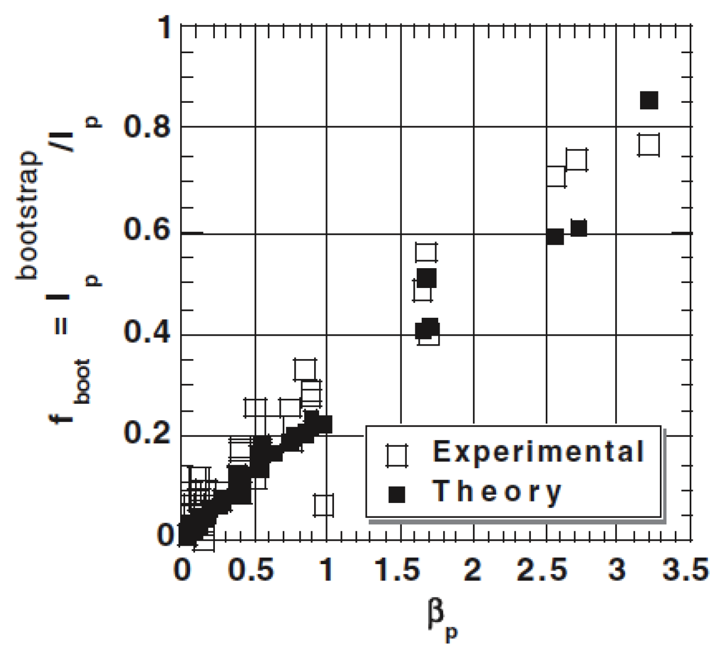
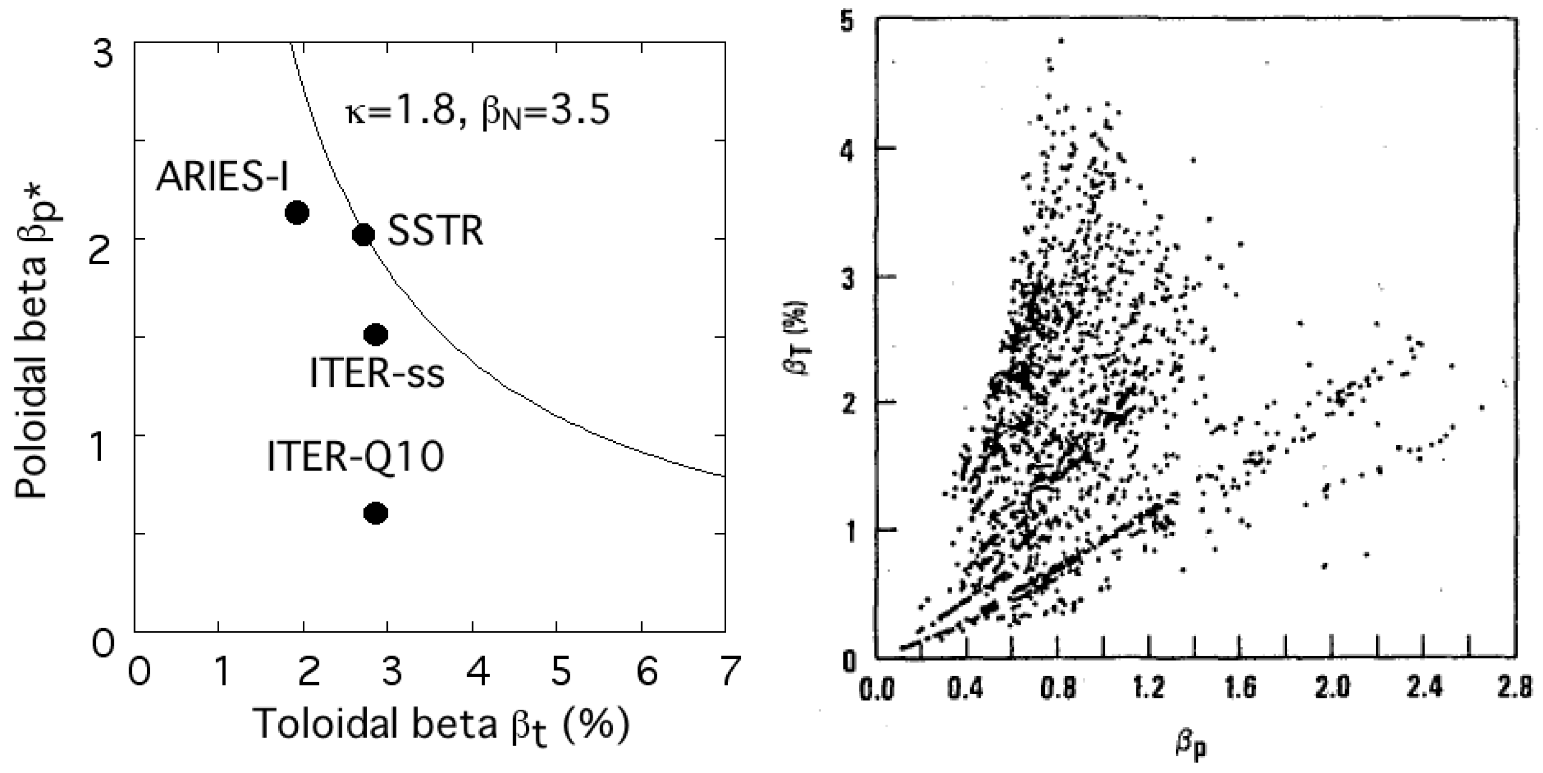
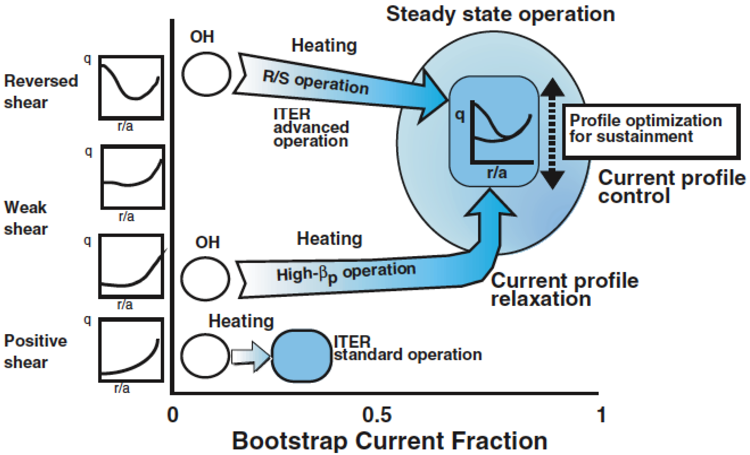
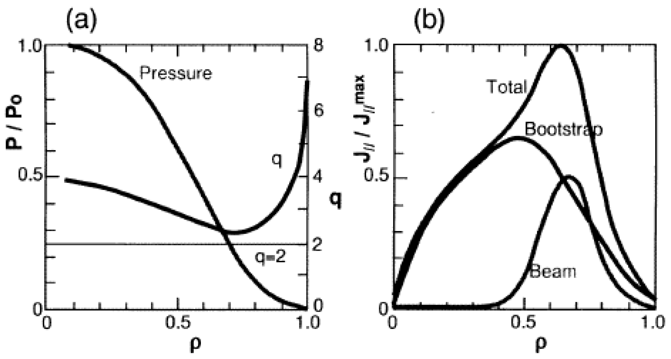
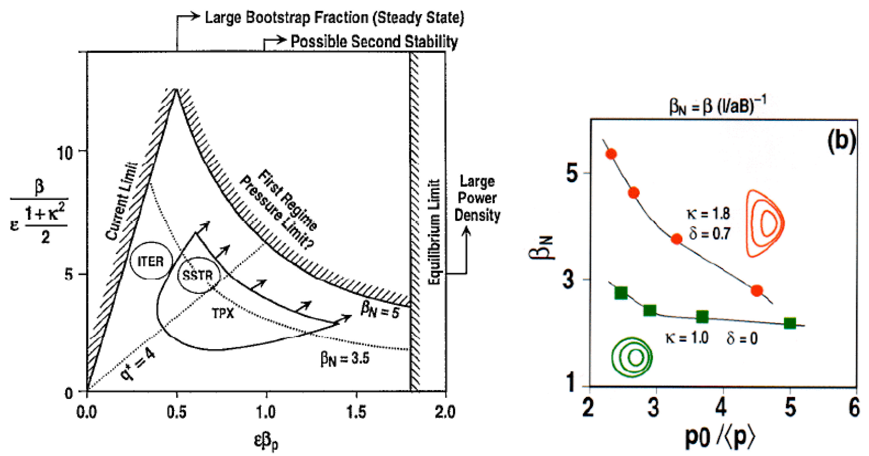
3.1. High Bootstrap and High Poloidal Beta Operation

The major feature of the efficient steady state operation of a tokamak is the maximum utilization of the bootstrap current. Since the bootstrap current fraction is proportional to the poloidal beta βp* = (4/(μ0Ip2Rp)∇PdV (or fboot~(a/R)0.5βp*,), the reactor should operate in a high βp* regime. This is a marked difference with high current and high toroidal beta research made before the initiation of the advanced tokamak research. The constraint on the plasma poloidal beta comes from the ideal and resistive MHD stability.The most important constraint is the so-called Troyon scaling described by Prof. F. Troyon in 1984 [81]:
βt = βNIp/aBt
where βN is a constant named “normalized beta”, βt = < P > /(Bt2/2μ0) is the volume averaged toroidal beta, Ip is the plasma current, a is plasma minor radius. The combination of Troyon scaling with the definition of poloidal beta βp* = (4/(μ0Ip2Rp)∇PdV gives the following relation:
β p * β t = κ 4 β N 2
where κ is vertical plasma elongation. Figure 12 shows the βp*t diagram in which the solid curve indicates the βp*t relation for κ = 1.8 and βN = 3.5 for reference. From equation (11), the toroidal beta βt is inversely proportional to βp* at a fixed βN. This scaling is confirmed most beautifully in DIII-D as shown in Figure 12 [82]. The regime corresponding to lower Ip and high q (typically q95~5) regime is called the advanced tokamak regime.
Figure 12. Nominal design points of ITER Q = 10 inductive operation (ITER-Q10), ITER steady-state operation (ITER-ss), SSTR and ARIES-I on a (βt, βp*) diagram, where reference line for βN = 3.5 and κ = 1.8. (left). Experimentally confirmed operating regime in (βp, βt) to confirm Troyon scaling in Doublet III (right) [82].
Energies 03 01741 g012
It is found in this figure that the steady-state fusion power concepts SSTR and ARIES-1 (βp* = 2 to 2.1) as well as the current ITER-ss design (βp*∼1.5) adopt high βp* operation to increase the bootstrap current fraction [8]. While a comprehensive theory of the bootstrap current is given later, a simple expression of the bootstrap current fraction is given by Cordey [83] as follows:
f b s = I b s I p = 0.67 ( a R ) 0.5 β p *
With current profile control, it is possible to achieve fbs~75% at βp*~2. This enables current drive of the remaining 25% of the plasma current by a high-energy beam or RF. It is important to notice that before 1990, world tokamak research was focused on increasing plasma current to improve energy confinement, typically represented by the design change from INTOR to ITER-CDA. Also, frontier research was directed towards achieving a high toroidal beta close to 10% with a highly normalized-current Ip/aBt in DIII-D [84].

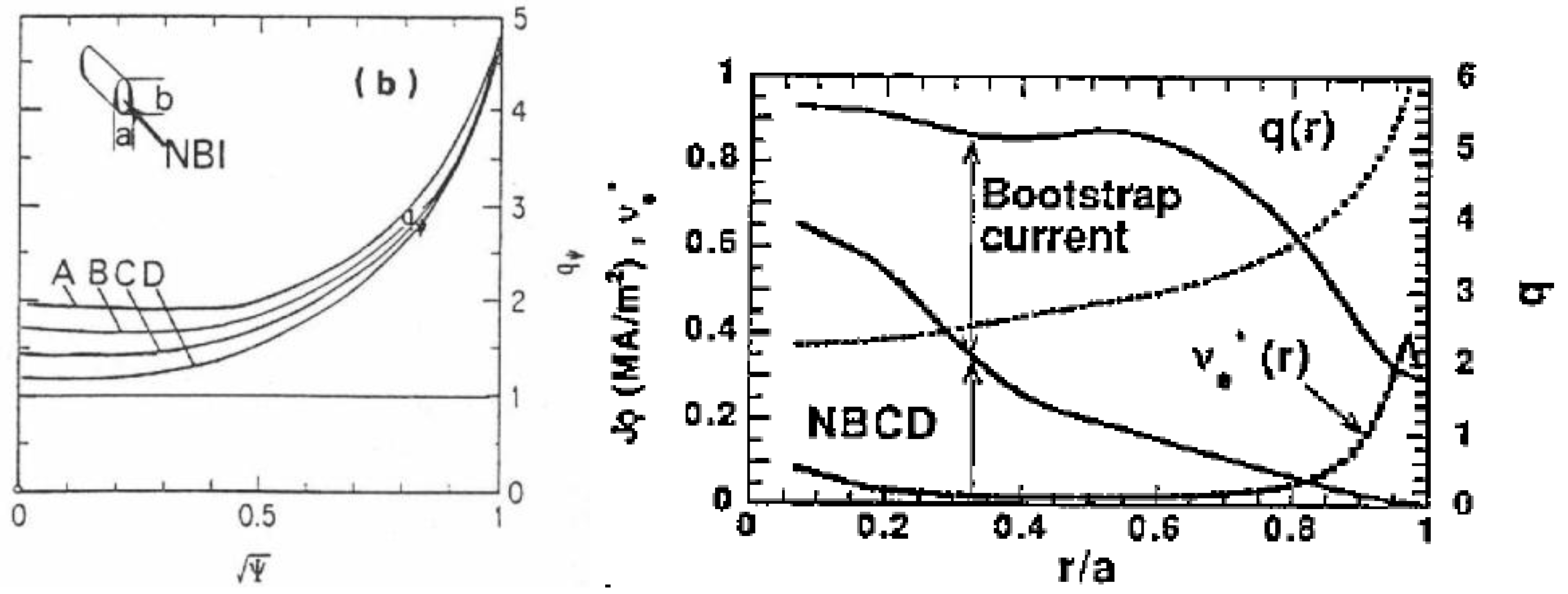
3.2. Current Profile Control of High Bootstrap Current Fraction Plasma

Since the bootstrap current has a hollow current profile, control of current profile is important for MHD stability and confinement improvement. Since the current profile is frozen and difficult to change when the plasma temperature becomes high, current profile control before intensive auxiliary heating is important. Access scenarios to advanced confinement regimes such as positive shear, weak shear and negative shear are shown in Figure 13.
Figure 13. Access to steady state operation regime with high bootstrap current fraction from OH regime. Since current profile is frozen at high temperature, current profile control in the target OH regime is important, according to Kishimoto [8].
Energies 03 01741 g013
One of important operational diagrams of a tokamak is the Cheng Diagram [85] or (q,li) diagram. Figure 14 shows the (q,li) diagram for JT-60U [86]. The low li boundary is limited by surface kink modes or locked mode while the upper li boundary is limited by tearing mode activities for low β regime. Advanced tokamak operation modes such as weak positive shear regime (or high βp regime) and reversed shear regimes are below the sawtooth boundary [87,88].
Figure 14. The (qeff, li) diagram in JT-60U showing the wide range of li explored in the experiments by Kamada [86]. Here, qeff ~0.8q95. High βN regime is characterized by relatively higher li and high βp regime is characterized by a relatively lower li below the sawtooth boundary [87].
Energies 03 01741 g014

3.3. Weak Positive Shear Regime

To eliminate the hollow current profile, an active central current drive with N-NBI was first proposed for the steady state operation with elevated q(0) to stabilize ballooning modes [5], now called weak positive shear regime, as shown in Figure 15. In this regime, improved core confinement is observed in high power neutral-beam heated large tokamaks such as JT-60U [87,88,89] and TFTR [90,91]. Ideal MHD stability of a weak shear regime was studied by Ozeki [78], showing that a SSTR relevant regime can be stable for ideal MHD modes with q(0) > 2 and wall stabilization.
Figure 15. Weak shear operation scenarios using central current drive by high energy N-NBI by Kikuchi [5].
Energies 03 01741 g015

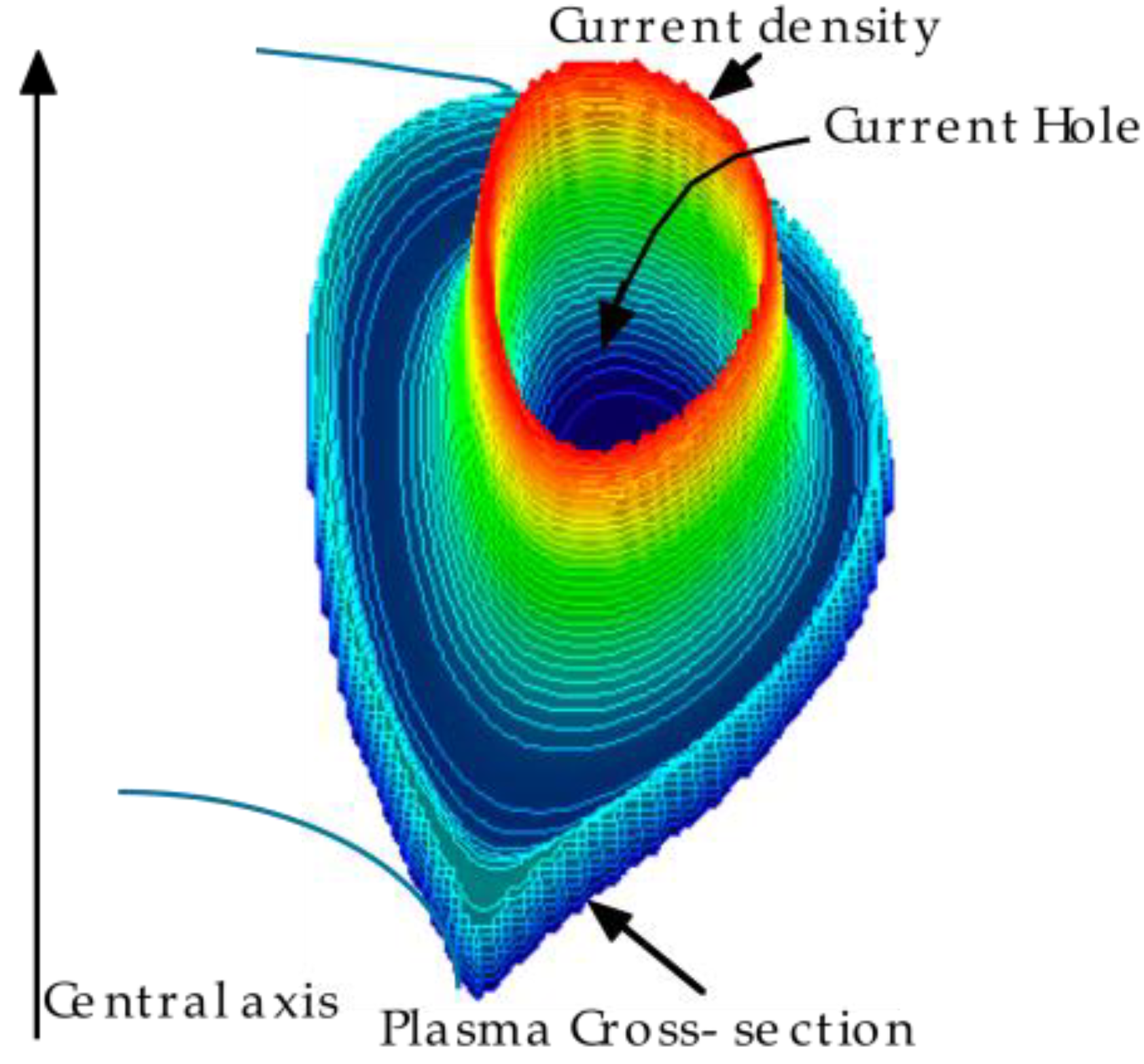
3.4. Negative Shear and Current Hole Regimes

After the SSTR proposal, Ozeki [92] found for the first time that a hollow current profile with peaked pressure profile and reduced pressure gradient near qmin can be stable for ideal MHD modes and this is called reversed shear operation or negative shear operation. He proposed to use the off-axis NBCD to realize a reversed shear profile as shown in Figure 16. Since the bootstrap current is a hollow current profile and has 1/Bp dependence, it is easier to obtain a higher bootstrap current fraction with a hollow current profile. Since then, many works have been done for optimization of the reversed shear scenario in both theory [93,94] and experiments in TFTR [95], DIII-D [96], and JT-60U [97]. To achieve a hollow current profile, a step-up scenario of PNB power during the current ramp-up (dIp/dt~0.5MA/s) is the key aspect to obtain a high electron temperature and to enhance the skin current effect. A key issue for stable evolution of an RS plasma is its stability when qmin passes through a low m/n rational surface. When the plasma current is ramped-up, qmin also decreases with time and may pass through a low m/n rational surface such as qmin = 4 and 3 and tends to disrupt at qmin = 2 due to beta collapse [98,99].
Figure 16. Negative shear operation scenario using off-axis current drive by Ozeki [92].
Energies 03 01741 g016
As an extreme situation in a negative shear configuration, equilibrium with zero plasma current in the central regime called “Current Hole” was formed in JT-60U [100] and JET [101], as shown in Figure 17. This current-hole regime can be stably sustained for a few seconds. This regime is interesting from the control viewpoint in that it has low li and is easier to get an elongated plasma and also is easier to get a high bootstrap current fraction. On the other hand, the Current Hole regime is subject to higher ripple loss and sets severe constraints on maximum toroidal field ripple as well as the low no-wall beta limit seen in negative shear regime.
Figure 17. Current Hole equilibrium in JT-60U observed by Fujita [101].
Energies 03 01741 g017

3.5. Advanced Tokamak Research

In 1993, the first comprehensive review on the prospects of the steady state tokamak reactor was given, which covered the physics requirements of a high bootstrap current fraction, confinement enhancement factors, non-inductive current drive, MHD stability including disruption probability, power and particle control and the need for new research directions was stressed, in addition to some engineering features of the magnet, neutral beam, coolant and material selection [102]. In 1994, Goldston [103] gave a talk on advanced tokamak physics in TPX design activity to establish the physics basis for the steady state tokamak. Since then, steady state tokamak research is called by the name of “Advanced Tokamak”.
Research directions have shifted to the demonstration of a high bootstrap high normalized-beta regime since the appearance of the SSTR concept. Especially, the establishment of a physics basis for steady state operation has becomes one of main research elements of JT-60U [14,15,16,17,18,19,20,21,25,26,27,28,29,30,31,32,33,34,35,36,37,38,39,46,47,48,49,50,51,52,53,54,55].
In 1997, Taylor [104] gave an EPS invited talk on the physics of advanced tokamaks, which is typically shown by the upper right regime in Figure 18 (left). This regime corresponds to a lower Ip and high q (typically q95~5) regime, which was called advanced tokamak regime. He surveyed improved confinement based on ExB shearing of microscopic turbulence and improved MHD stability to achieve higher βN using shaping and pressure profile control, as shown in Figure 18 (right). Ozeki also addressed the physics issues of high bootstrap current tokamaks, including TAE stability in EPS [105]. Recent DIII-D advanced tokamak experiments show 100% noninductive plasma with βt = 3.6%, βN = 3.5, H89 = 2.4[106].
Figure 18. Advanced tokamak operating regime (left) and shape and profile effect on normalized beta (right) [104].
Energies 03 01741 g018

4. Parallel Collisional Transport Physics for Steady State Tokamak Operation

Since plasma current plays an essential role in tokamak confinement, it is quite important to understand the parallel transport physics, especially generalized Ohm’s law. Fortunately, most of the parallel transport in a tokamak is governed by the collisional transport and we have developed Matrix Inversion (MI) Method [73] based on the Hirshman-Sigmar neoclassical transport theory [107].

4.1. Moment Equation

As Hirshman and Sigmar [107] showed, we obtain the following moment equations for momentum and heat flux by taking v and v2v moments of Vlasov-Fokker Planck equation of species a after subtracting convective heat flux from the v2v moment:
m a n a d u a d t = e a n a ( E + u a × B ) P a a + F a 1 + M a
m a t ( q a T a ) = e a T a q a × B 5 2 n a T a Θ a + F a 2 + Q a
Here, na, ua, qa, Pa, a, Θa, Fa1, Fa2, Ma, Qa are density, velocity, conduction heat flux, the average plasma pressure, viscosity tensor (anisotropic component of the pressure) and viscous heat tensor, friction force, heat friction force, momentum source, and heat momentum source, respectively. Velocity distribution function in strong magnetic fields shows anisotropy parallel and perpendicular to the magnetic field, as shown by Chew, Goldberg, and Low [108], and a and Θa can be expressed as:
a = ( P / / a P a ) ( b b 1 3 I ) + O ( δ 2 )
Θ a = ( Θ / / a Θ a ) ( b b 1 3 I ) + O ( δ 2 )
Here, b = B/B is the unit vector parallel to B and δ = ρa/L is a smallness parameter as a ratio of Larmor radius and the macroscopic length scale L of the plasma, ρa = vTaa is the Larmor radius, vTa = (2Ta/ma)1/2 is the thermal velocity, Ωa = eaB/ma is the cyclotron angular frequency. Taking the cross product B with (10) and (14), and neglecting the time derivative for the drift time scale O((δ2Ω)‑1) much longer than the Alfven time scale O((δΩ)−1), and neglecting other O(δ2) terms smaller than ∇P, ∇Φ, ∇T terms, the major components of particle and heat flows of particle species a perpendicular to B are given as:
u a ( 1 ) = E × B B 2 + b × P a m a n a Ω a
q a ( 1 ) = 5 2 P a b × T a m a Ω a
Here, first term of rhs of (17) is the ExB drift flow, the second term is the diamagnetic drift flow caused by the pressure gradient. Equation (18) is the diamagnetic heat flux caused by the temperature gradient. On the drift time scale, −∂A/∂t term is negligible and we can write E = −∇Φ. Taking the dot product of the magnetic field B with (13) and (14) and taking the flux surface average, following flux surface averaged momentum and heat flux balance equation are obtained:
B a = B F a 1 + e a n a B E + B M a
B Θ a = B F a 2 + B Q a
Here B F a 1 and B F a 2 are the frictional forces on species a by the parallel flow on the magnetic surface, and B a and B Θ a are viscous forces parallel to B, which originate from the relaxation of velocity space anisotropy between parallel and perpendicular to B. Substitution of (15) and (16) gives following equations:
B a = ( P / / a P a ) b B
B Θ a = ( Θ / / a Θ a ) b B
In 1995, a comprehensive review on the experimental evidence for the bootstrap current was given [109]. In this paper, the origin of this velocity space anisotropy is pictorially explained in case of the electron as in Figure 19. The magnetic moment μ is conserved in a high temperature plasma when the electron moves along the magnetic field. So, the orbit of the electrons satisfying Bmax ≥ E/μ is trapped in the weak magnetic field regime reflected by the magnetic mirror (trapped particle orbit: or called “Banana Orbit” from its shape). Consider the case density is lowering towards the outside (dn/dr < 0). Consider the velocity distribution function in a magnetic surface. There are less electrons for the trapped electrons with v// > 0 since it comes radially from outside, while there are more electrons for the trapped electrons with v// < 0 since it comes radially from inside. Meanwhile, the orbit of un-trapped electrons stays much closer to the magnetic surface and the number of electrons for v// > 0 is roughly equal to that for v// < 0. Then, there appears a discontinuity in the trapped/un-trapped boundary of the velocity distribution function. Small Coulomb collision smoothes this gap and causes the particle diffusion in the velocity space. This collisional diffusion in velocity space acts as a viscous force in the magnetic field direction.
Figure 19. Sketch of the trapped electron orbits and distortion of one and two dimensional velocity distribution functions in a tokamak showing how collisional diffusion acts at trapped-passing boundary [109].
Energies 03 01741 g019

4.2. Flux surface Averaged Momentum and Heat Flow Balance

The friction and heat friction forces in (19) and (20) are given by:
[ F a 1 F a 2 ] = b ( l 11 a b l 12 a b l 21 a b l 22 a b ) [ u b ( 1 ) 2 q b ( 1 ) / 5 P b ]
Here, l i j a b is called the friction coefficient, which has the symmetry l i j a b = l j i b a due to self-adjoint property of the Coulomb collision term:
l i j a b = m a n a τ a a [ ( k τ a a τ a k M a k i 1 , j 1 ) δ a b + τ a a τ a b N a b i 1 , j 1 ]
M a b 00 = ( 1 + m a m b ) ( 1 + x a b 2 ) 3 / 2 ,   M a b 01 = 3 2 ( 1 + m a m b ) ( 1 + x a b 2 ) 5 / 2 ,
M a b 11 = ( 13 4 + 4 x a b 2 + 15 2 x a b 4 ) ( 1 + x a b 2 ) 5 / 2
N a b 00 = ( 1 + m a m b ) ( 1 + x a b 2 ) 3 / 2 ,   N a b 10 = 3 2 ( 1 + m a m b ) ( 1 + x a b 2 ) 5 / 2 ,
N a b 01 = 3 2 T a T b x a b 1 ( 1 + m a m b ) ( 1 + x a b 2 ) 5 / 2 ,   N a b 11 = 27 4 T a T b x a b 2 ( 1 + x a b 2 ) 5 / 2
τ a b = 3 π 3 / 2 ε 0 2 m a 2 v T a 3 n b e a 2 e b 2 ln Λ ,   x a b 2 = m a T b m b T a , v T a = 2 T a m a
Here, the friction coefficient has the following symmetry due to the self-adjointness of the Coulomb collision operator:
l i j a b = l j i b a ,   M a b i j = M a b j i ,   N a b j 0 = M a b j 0 ,   N a b i j = T a v T a T b v T b N b a j i
Since viscous force operates when the particle moves poloidally to feel the variation of the toroidal field, the viscous force is proportional to the poloidal flows:
[ B a B Θ a ] = B 2 [ μ a 1 μ a 2 μ a 2 μ a 3 ] [ u a θ * ( ψ ) 2 q a θ * ( ψ ) / 5 P a ]
Here, μa1, μa2, μa3 are called parallel viscosity coefficients. Collisional transport regimes in tokamak are divided into three regimes: (1) Banana regime where the collision time is longer than the bounce time of trapped particle orbit (νc < Ωb; νc: collision frequency, Ωb: bounce frequency), (2) Pfirsh-Schlüter regime where the collision time is shorter than the transit time of the un-trapped particle (νc > Ωt; νc: collision frequency, Ωt: transit frequency ~vTa/Rq), (3) plateau region between the two. Expression of the viscosity coefficient is derived for each regime and the velocity partitioned approximate viscosity coefficient valid for all velocity region is derived. The viscosity coefficient is obtained by the integration in the velocity space as follows:
μ a 1 = K 11 a
μ a 2 = K 12 a 5 2 K 11 a
μ a 3 = K 22 a 5 K 12 a + 25 4 K 11 a
where:
K i j a = m a n a τ a a f t f c { x a 2 ( i + j 2 ) ν t o t a ( v ) τ a a }
{ A ( v ) } = 8 3 π 1 / 2 0 exp ( x a 2 ) x a 4 A ( x a v a ) d x a
ν t o t a ( v ) = ν D a ( v ) [ 1 + 2.48 ν a * ν D a ( v ) τ a a / x a ] [ 1 + 1.96 ν T a ( v ) / x a ω T a ]
ν T a ( v ) = 3 ν D a ( v ) + ν E a ( v ) , x a = v / v T a , ω T a = v T a / L c
Here, first term of the denominator of (33) is the correction term to connect the banana and plateau regimes, while the second term is the Pfirsh-Schlüter correction term. xa = v/vTa, ν D a ( v ) is 90-degree deflection frequency, ν E a ( v ) energy exchange frequency. Collision frequencies ν D a ( v ) and ν E a ( v ) in the expression of the viscosity coefficient for Maxwellian is expressed as follows:
ν D a ( v ) = 3 π 4 1 τ a a b n b Z b 2 n a Z a 2 Φ ( x b ) G ( x b ) x a 3
ν D a ( v ) = 3 π 4 1 τ a a b n b Z b 2 n a Z a 2 [ 4 ( T a T b + x a b 2 ) G ( x b ) x a 2 Φ ( x b ) x a 3 ]
Φ ( x ) = 2 π 0 x exp ( u 2 ) d u , G ( x ) = [ Φ ( x ) x Φ ( x ) ] / 2 x 2
Also, νa* is the collisionality defined by the ratio of collision frequency 1/τaa, the transit frequency ωTa, and ε(ψ) ≡ (Bmax-Bmin)/(Bmax + Bmin). Using connection length Lc~Rq and ε~r/R:
ν a * 1 ε 1.5 ω T a τ a a ~ ( R r ) 1.5 R q v T a τ a a
Here, ft is a trapped particle fraction and is related to un-trapped particle fraction fc through ft + fc = 1. The fc is given by the following equation:
f c = 3 B 2 4 0 1 / B m a x λ d λ 1 λ B
Substituting these formulas for viscosity and friction coefficients into (19) and (20), following balance equation of friction and viscous forces are obtained:
[ μ a 1 μ a 2 μ a 2 μ a 3 ] [ B u / / a B V 1 a 2 B q / / a / 5 P a B V 2 a ] = b [ l 11 a b l 12 a b l 21 a b l 22 a b ] [ B u / / b 2 B q / / b / 5 P b ] + [ e a n a B E / / 0 ] + [ B M a / / B Q a / / ]
Here, μai, lijab, u//a, q//a, Ma//, Q//a, Via (BV1a = −F(ψ)(dΦ/dψ + (dPa/dψ)/eana), BV2a = −F(ψ)(dTa/dψ)/eana, and Φ is electrostatic potential) are viscosity coefficient, friction coefficient, parallel flow, parallel heat flow, parallel momentum source, parallel heat source, thermodynamic forces, respectively.

4.3. Generalized Ohm’s Law

The following system of linear equations is obtained by writing down (39) for electrons, ions, and impurities [109]:
M ( U / / V ) = L U / / + E * + S / /
Here, M, L, U//, V, E*, S// are viscosity matrix, friction matrix, parallel flow vector, thermodynamic force vector, electric field acceleration vector, parallel source vector, and given as follows:
M = [ μ e 1 0 0 0 μ i 1 0 0 0 μ I 1 μ e 2 0 0 0 μ i 2 0 0 0 μ I 2 μ e 2 0 0 0 μ i 2 0 0 0 μ I 2 μ e 3 0 0 0 μ i 3 0 0 0 μ I 3 ] ,   L = [ l 11 e e l 11 e i l 11 e I l 11 i e l 11 i i l 11 i I l 11 I e l 11 I i l 11 I I l 12 e e l 12 e i l 12 e I l 12 i e l 12 i i l 12 i I l 12 I e l 12 I i l 12 I I l 21 e e l 21 e i l 21 e I l 21 i e l 21 i i l 21 i I l 21 I e l 21 I i l 21 I I l 22 e e l 22 e i l 22 e I l 22 i e l 22 i i l 22 i I l 22 I e l 22 I i l 22 I I ]
U / / = [ B u / / e B u / / i B u / / I 2 B q / / e / 5 P e 2 B q / / i / 5 P i 2 B q / / I / 5 P I ] ,   V = [ B V 1 e B V 1 i B V 1 I B V 2 e B V 2 i B V 2 I ] , E * = B E / / [ e n e e Z i n i e Z I n I 0 0 0 ] ,   S / / = [ B M e B M i B M I B Q e B Q i B Q I ]
Solving (40) for U// gives:
U / / = ( M L ) 1 M V + ( M L ) 1 E * + ( M L ) 1 S / /
Then, plasma current density parallel to the magnetic field is expressed in the following form and is called generalized Ohm’s law:
B J = B J b s + σ / / N C B E + B J N B C D + B J R F C D
Here terms on the right hand side are called bootstrap current, ohmic current, beam and RF driven currents, respectively and are given as follows:
Energies 03 01741 i001
Energies 03 01741 i002
σ / / N C B E = a = e , i , I e a n a { b = 1 3 [ ( M L ) 1 ] a b e b n b B E }
B J N B C D + B J R F C D = a e a n a { b [ ( M L ) 1 ] a b S / / b }

4.4. Electrical Conductivity

The inductive operation is quite effective to drive the plasma current since the electrical conductivity of high temperature plasma (e.g., σ = 109/ohm-m for Te = 10 keV) is 20 times larger than that of copper (e.g., σ = 5 × 10⁷/ohm-m at room temperature). From equation (45), we obtain the expression of electrical conductivity σ (fast ion contribution is neglected):
σ / / N C = a = e , i , I b = e , i , I e a n a e b n b [ ( M L ) 1 ] a b
Here, L represents the collisional friction forces among various species, and M represents effect of trapped particle. If there is no trapped particles, the viscosity matrix M = 0 and conductivity σ is given in this case as follows:
σ / / S p i t z e r = a = e , i , I b = e , i , I e a n a e b n b L 1 a b
which is called “Spitzer conductivity”. The electrical conductivity is reduced by viscosity M. The trapped particle is trapped in the banana orbit as shown in Figure 19 and does not contribute to the current. It creates a frictional force by the velocity relative to un-trapped electrons, which are drifting by the electric field. The electrical conductivity given by L. Spitzer Jr. [110] agrees well with the numerical value from this expression:
σ / / S p i t z e r = n e e 2 τ e e m e 3.4 ( 1.13 + Z e f f ) Z e f f ( 2.67 + Z e f f )
Z e f f = 1 n e b = i , I n b Z b 2 ,   τ e e = 6 2 π 3 / 2 ε 0 2 m e 1 / 2 T e 3 / 2 n e e 4 ln Λ = 2.74 x 10 4 T e [ k e V ] 3 / 2 n e [ m 3 ] ln Λ [ sec ]
Here, Zeff is the effective charge. Hirshman [111] also gave an approximate analytic expression for electrical conductivity as follows:
σ / / N C = σ / / S p i t z e r [ 1 f t 1 + ξ ν e * ] [ 1 C R f t 1 + ξ ν e * ]
C R ( Z e f f ) = 0.56 Z e f f 3 Z e f f 3 + Z e f f , ξ ( Z e f f ) = 0.58 + 0.2 Z e f f
f t = 1 ( 1 ε ) 2 ( 1 + 1.46 ε 1 / 2 ) 1 ε 2
Here, the trapped particle fraction ft (54) is not accurate enough for a non-circular cross-section plasma and in such a case (38) must be used.

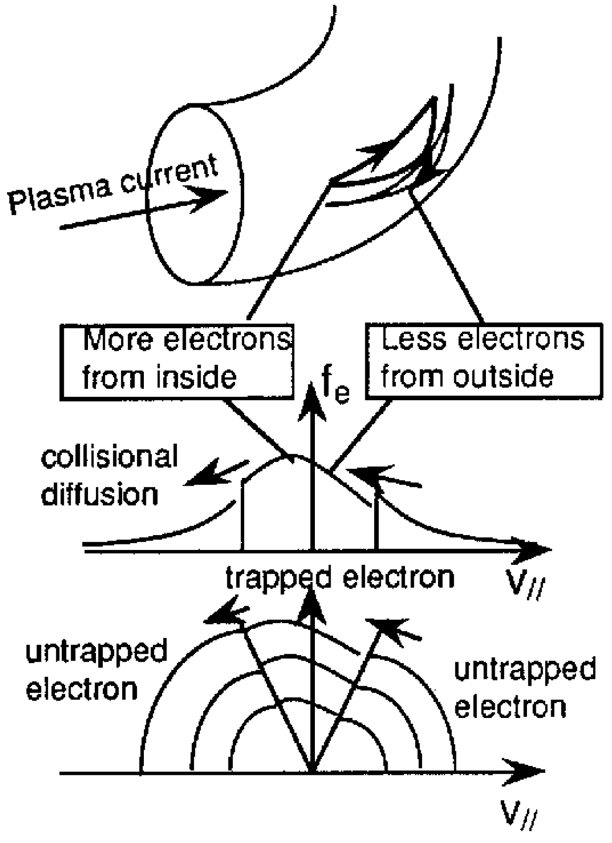
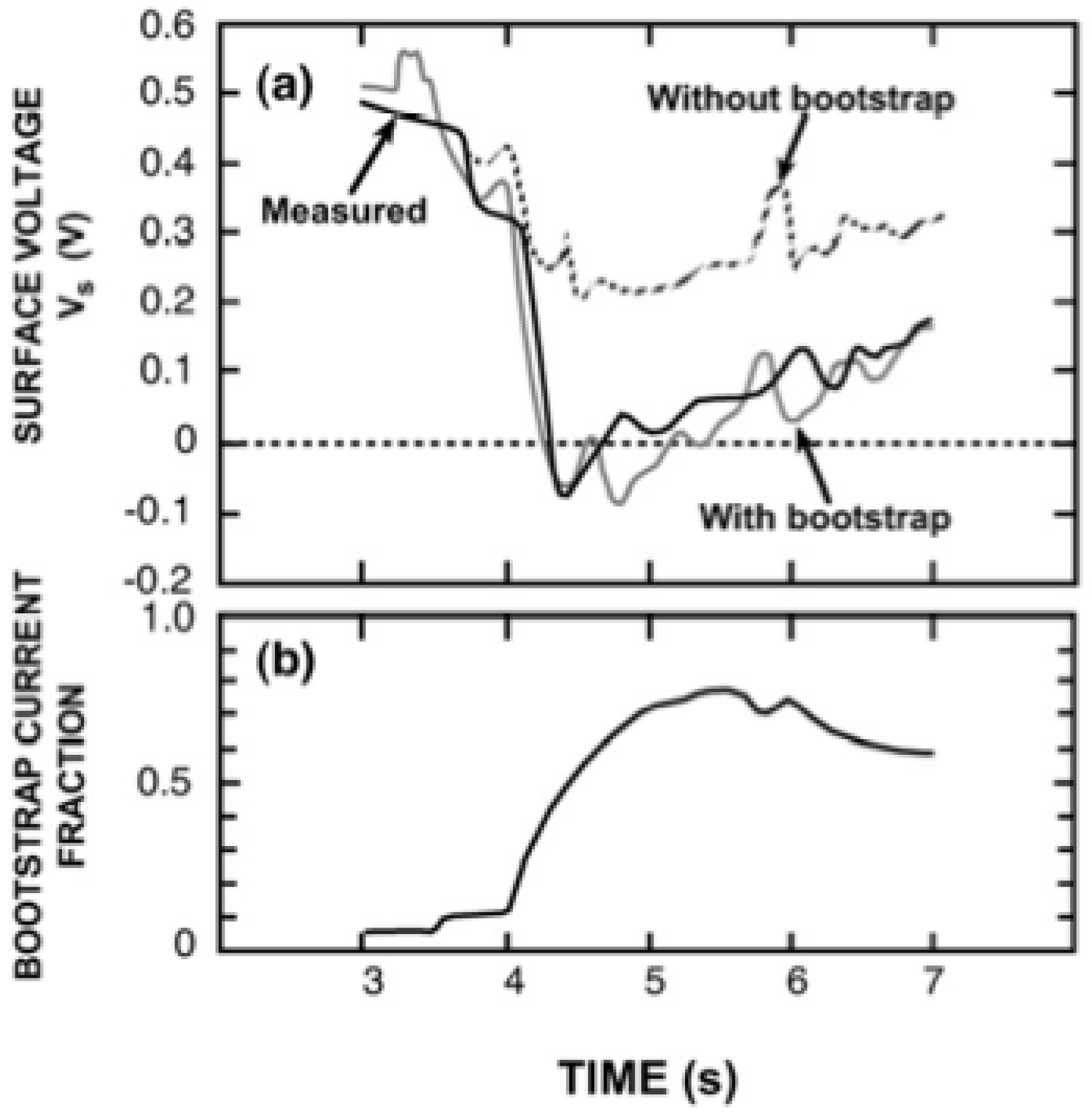
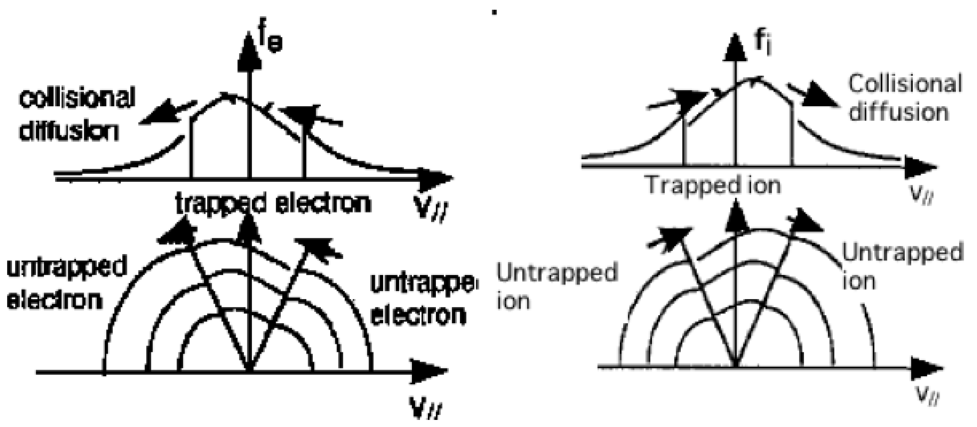
4.5. Bootstrap Current

The generalized Ohm’s law in (42) includes current driven by the thermodynamic forces V1a and V2a (BV1a = −F(ψ)(dΦ/dψ + (dPa/dψ)/eana), BV2a = −F(ψ)(dTa/dψ)/eana) as follows:
B J b s = a = e , i , I e a n a b = 1 6 α a b V b
where matrix α is defined as α = (ML)−1M. Substituting expressions for thermodynamic forces V1a and V2a into (55), we obtain following form for the bootstrap current:
Energies 03 01741 i003
Energies 03 01741 i004
Although V1a includes an electrostatic potential term, this term ( J ~ F ( Z b n b α b a ) d Φ / d ψ ) vanishes for the axisymmetric plasma due to charge neutrality. Distortion of the velocity distribution function occurs in collision-less plasma. The electron distribution function is drifting in the direction of v// < 0 while the ion velocity distribution function is drifting in the direction of v// > 0, as seen in Figure 20. This produces the plasma current and is named bootstrap current.
Figure 20. Sketch of the mechanism of the bootstrap current in a collisionless plasma for electrons and ions. Collisional pitch angle scattering at the trapped-untrapped boundary produces an unidirectional parallel flow/momentum input and is balanced by the collisional friction force between electrons and ions. The source of the momentum input for parallel flow drive is radially outward motion/loss of trapped particles.
Energies 03 01741 g020
Let's look at the role of the viscosity coefficient for the expression of the bootstrap current in a simple model. When we ignore the ion and impurity flows (ui = uI = 0), the electron momentum balance equation (39) becomes as follows:
μ e 1 ( u / / e R e n e d P e d ψ ) = l 11 e e u / / e
So, the electron bootstrap current is given by:
J e b s = e n e u / / e = R μ e 1 μ e 1 l 11 e e d P e d ψ = μ e 1 μ e 1 l 11 e e 1 B p d P e d r
Figure 21 shows a comparison of plasma surface voltages between measurement and 1.5 dimensional transport simulation (called so by the coupling of two dimensional equilibrium and one dimensional current diffusion transport simulation) using the measured plasma parameters. If we do not include bootstrap current in the transport simulation, the simulation does not reproduce the measurement and the existence of the bootstrap current is confirmed [109].
Figure 21. Comparison of time variation of measured surface voltage and simulation using (42) of JT-60 discharge [109]. Up to 80% of the plasma current is carried by the bootstrap current from the simulation. Without including bootstrap current, the measured surface voltage can’t be reproduced.
Energies 03 01741 g021

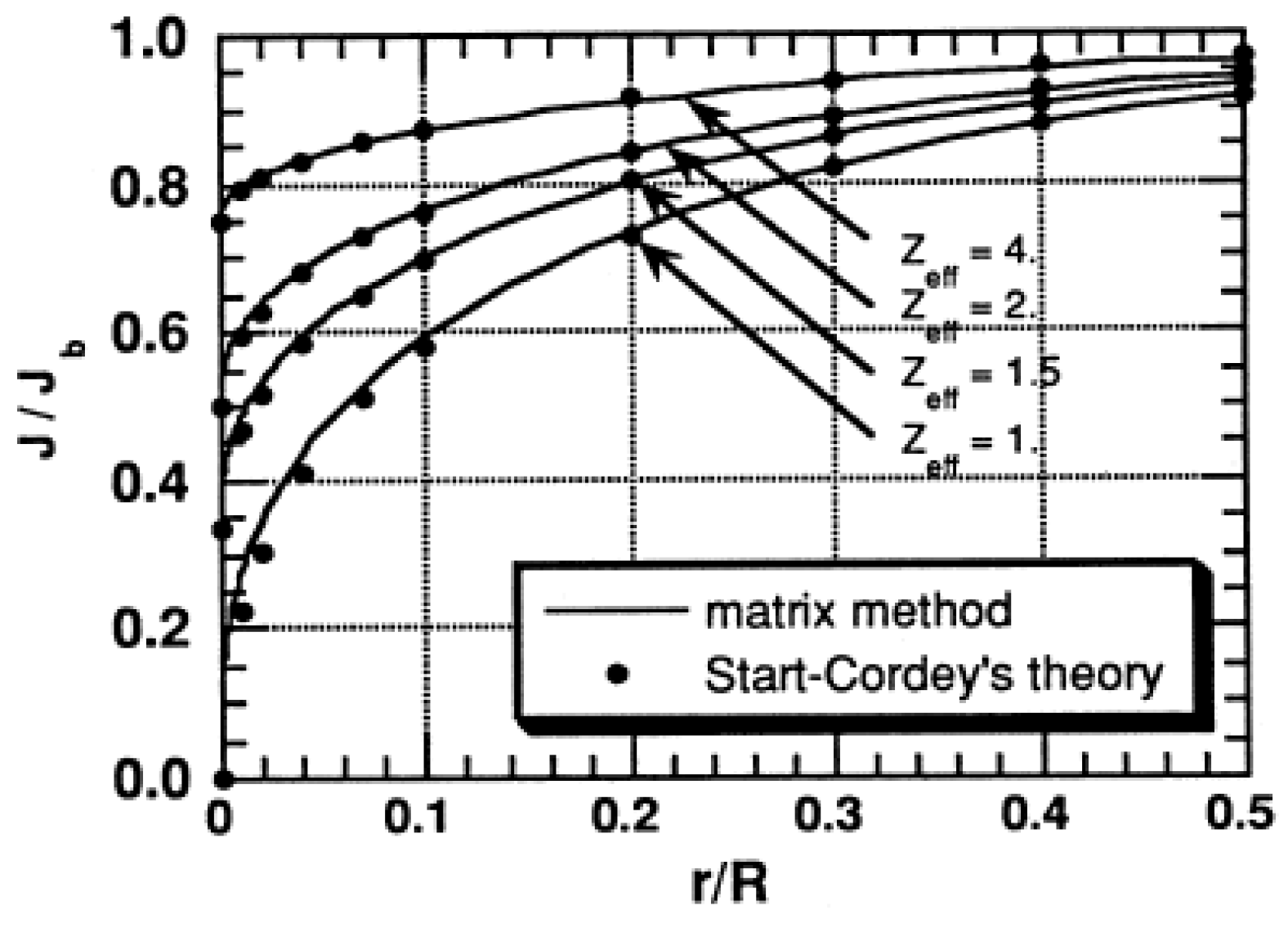
4.6. Neutral Beam Current Drive [112]

4.6.1. Neutral Beam Current Drive Theory

When a fast neutral beam is injected tangentially to the torus, circulating fast ions produce a fast ion current by multiple circulations around the torus. Collision with bulk electrons produces a shielding current by induced drift in the same direction as the fast ions. This shielding is not perfect due to the existence of trapped electrons and impurities. The sum of the fast ion and shielding currents is called beam-driven current Jbd, which is a current in response to the external momentum source S//a given in (40) but momentum balance of fast ion has to be included as follows [109]:
B J b d = a = e , i , I , f e a n a [ ( M L ) 1 ] a f S / / f
Here, ea, na, M and L are electrical charge, density, viscous and friction matrixes including fast ion momentum balance equation, respectively and S//f is momentum source from fast ion. So, if we divide the beam driven current into fast ion current and shielding current B J b d = B J f a s t + B J s h i e l d , we obtain:
B J f a s t = e f n f [ ( M L ) 1 ] f f S / / f
B J s h i e l d = a = e , i , I e a n a [ ( M L ) 1 ] a f S / / f
F = B J b d B J f a s t = a = e , i , I , f e a n a [ ( M L ) 1 ] a f e f n f [ ( M L ) 1 ] f f
where, eb, nb Sb are electrical charge, density and momentum source density of beam ion, respectively. Also, F is called stacking factor. Parametric dependences of F on Zeff and e in arbitrary aspect ratio (0 ≤ ε ≤ 1) are calculated by (18) and shown in comparison with Start-Cordey calculation [113] in Figure 22.
Figure 22. Stacking factor F for neutral beam current drive as a function of r/R and Zeff [109] in comparison with Calculation by Start-Cordey [113].
Energies 03 01741 g022
To evaluate the fast ion current < B ⋅ J > fast, we have to solve the fast ion Fokker-Planck equation for the velocity distribution function of fast ions fb valid for vTi ≤ vb ≤ vTe. Fast ion Fokker-Planck equation in non-uniform magnetic field is give by Connor [114]:
τ s f b t = v 2 v [ ( v c 3 + v 3 ) f b ] + β v c 3 v 3 η v / v / / η [ ( 1 η 2 ) η v / / v f b η ] + τ s S ( v , η )
τ s e = 3 ( 2 π ) 3 / 2 ε 0 2 M b T e 3 / 2 e 4 Z b 2 n e m e 1 / 2 ln Λ ,   E c = ( 9 π m p 16 m e ) 1 / 3 [ j n j Z j 2 n e A j ] 2 / 3 A b T e
where, tse is beam-electron slowing down time, Ec is the critical energy, vc is critical velocity defined by vc = (2Ec/mb)1/2, vb is the beam velocity (= (2Eb/mb)1/2), β is defined by β = ZeffnelnΛe/2mbΣmj-1Zj2lnΛi, S(v,η) is the bounce averaged fast ion source rate per unit volume, Zeff is the effective charge defined by Zeff = ΣjnjZj2/ne, < v/v// > is given by < v/v// > = (2/π)K[(ηt/η)2] and < v///v > are given by < v///v > = (2/π)E[(ηt/η)2] for passing ions, where K and E are complete elliptic integrals of 1st and 2nd kind, respectively. The η is defined by η = (1 − μBmin/E)1/2, where m = mbv2/2B is the magnetic moment. The η value at trapped-passing boundary ηt is given by ηt = (1 − Bmin/Bmax)1/2, where Bmax is the maximum total magnetic field on the magnetic surface, usually at the inboard side of the torus. The solution of (64) is given in J. Cordey [115] as follows:
f b ( v , η ) = S 0 τ s e n a n ( v ) c n ( η )
where, an(v) is the analytical solution for uniform magnetic field by Gaffey [116]:
a n = k n v 3 + v c 3 [ v 3 ( v b 3 + v c 3 ) v b 3 ( v 3 + v c 3 ) ] β λ n / 3    v v b = k n v b 3 + v c 3 exp [ 2 E b ( 1 + ( v c / v b ) 3 T e + ( v c / v b ) 3 T i v v b v b ]    v v b
Here, S(v, η) = S0δ(v − vb)k(η) = S0δ(v − vb)Σkncn(η) and fast ion distribution function above beam energy (v > vb) comes from energy diffusion in velocity space. The following equation determines the eigen-value ln and eigen-function cn(η):
1 η v / v / / η [ ( 1 η 2 ) v / / v c n η ] + λ n c n = 0
This equation is solved numerically by the Rayleigh-Ritz method in the ACCOME code [117]. Using above formulas, the flux surface averaged parallel fast ion current multiplied by B, < B ⋅ J > fast can be calculated as:
B J f a s t = e Z h 0 v 3 d v 1 1 d η f b ( v , η , ρ ) H ( v , η , ρ )
H ( v , η , ρ ) = B d s v d s v / /
The dependence of the current drive efficiency h = Jbd/SEb0 on Te and ne are given as follows by taking τse~Te1.5/ne and Eb0/vb0~vb0~(vb0/vc)vc, vc~Te0.5:
h ( T e , n e ) = J b d S E b 0 = F J f a s t S E b 0 ~ τ s e v b 0 E b 0 f 0 ( E b 0 / E c ) ~ τ s e v c f ( E b 0 / E c ) ~ T e n e f ( E b 0 / E c )
where f(x) = f0(x)/x1/2.

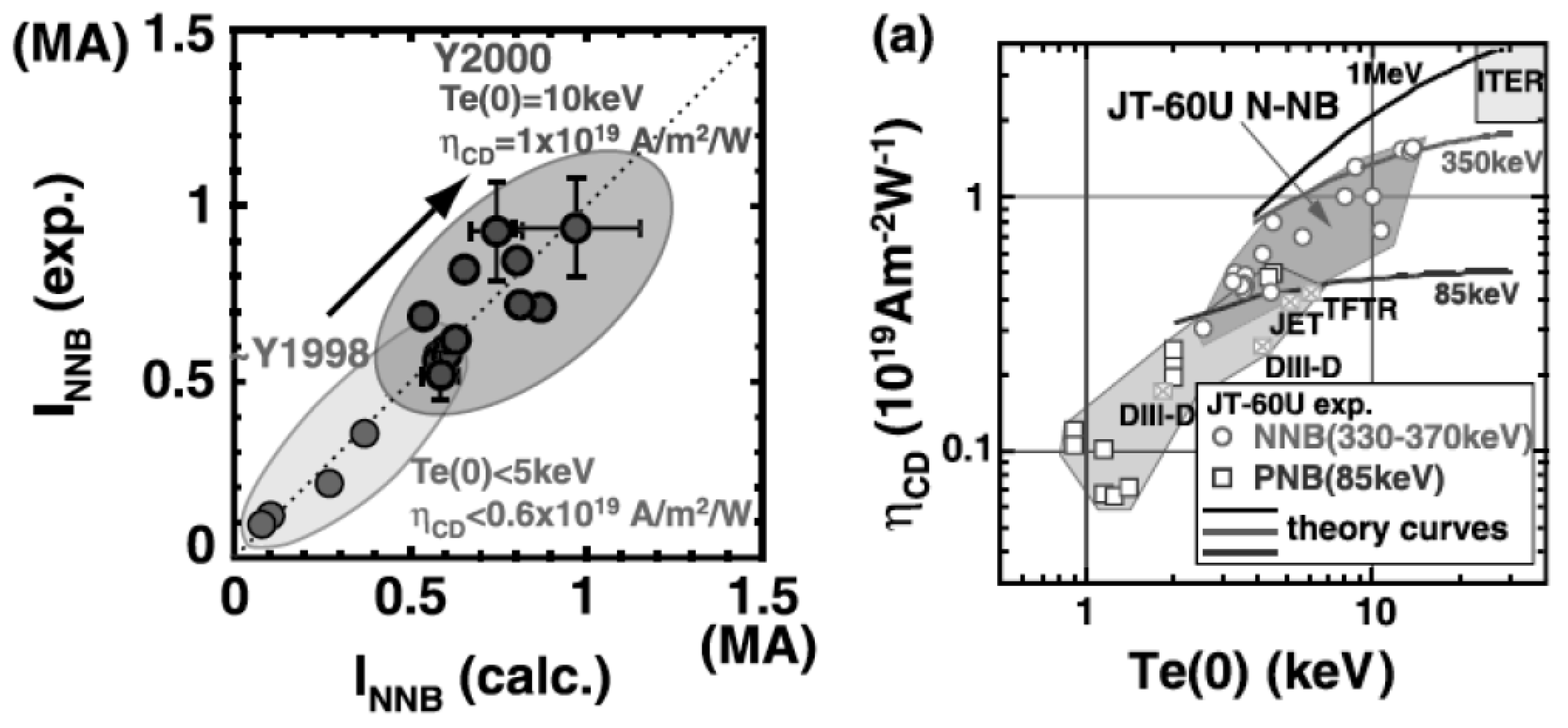
4.6.2. Demonstration of Current Drive with N-NBI

The SSTR design utilizes high energy neutral beam injection for the non-inductive current drive. Therefore it is necessary to demonstrate the effectiveness of heating and current drive by high energy neutral beam for the ITER and the steady state tokamak reactor.
Figure 23. Bird’s eye view of N-NBI injector and JT-60U tokamak.
Energies 03 01741 g023
Consequently, the first world project to install a 500 keV negative ion based neutral beam injection system (N-NBI) was started in JT-60U to demonstrate its feasibility [118]. Key advantages of N-NBI are: (1) the ability to place the injector far from the reactor for easy maintenance, (2) no accessibility issues across the plasma boundary, (3) robustness against plasma conditions, especially no dependence on the toroidal field, (4) high energy conversion efficiency using a gas neutralizer or plasma neutralized for the reactor, (5) acceptable current drive efficiency η = < ne > RIpCD/PCD = 5 × 10¹⁹A/W/m2. Figure 23 shows a bird’s eye view of the N-NBI system in JT-60U, which started operation in 1996 [15].
Table 1 shows the major specifications of the N-NBI system in JT-60U [118]. Since then, progress has been made to increase beam voltage by conditioning [119], to improve ion source uniformity [120,121] and to reduce heat load to the electrodes [122,123].
Table 1. Design specification of JT-60U N-NBI system [118].
ItemValueItemValue
Designed Beam Energy500keVBeam speciesD/H
Injection Power10MWIon sourceCs seeded multi-cusp
Beam duration10sFilament materialW
Current drive efficiency was extensively investigated for a range of beam energies (≤350 keV) and electron temperatures (Te ≤ 14 keV) much wider than in previous experiments [124]. A method to calculate plasma equilibrium with inductive and non-inductive (beam-driven and bootstrap) currents is established in numerical codes such as ACCOME [117]. A method of experimental determination of non-inductively driven current was established by Forest [125]. Ohm’s law in a general toroidal geometry without bootstrap current and RFCD is given by:
B J = σ / / N C B E + B J N B C D
where the electric field is related to the time variation of poloidal flux at constant F surface as follows:
B E = B φ 2 F ψ t | Φ
Time evolution of the poloidal flux ψ(r, t) and < B·J > can be measured by the MSE diagnostics with equilibrium magnetic fitting code such as EFIT [126]. By calculating the Ohmic current using measured ∂ψ/∂t, density, temperature and Zeff profiles, non-inductively driven current < B·J> NBCD can be “measured” as difference < B·J > NBm = < B·J > − σ//NC < B·E >. This current density profile can be compared with the numerical calculation of < B·J > NBc using measured density, temperature and Zeff profiles. A comparison is shown in Figure 24. It is worth noting that calculated and “measured” non-inductively driven current profiles agree with each other when multi-step ionization effect is taken into account in the calculation of < B·J > NB.
Theoretical NB current drive efficiency increases with electron temperature Te in Equation (70). This dependence is also confirmed experimentally, as shown in Figure 24. Maximum NBCD efficiency hCD = 1.55 × 10¹⁹A/W/m2 is achieved at Te(0) = 14 keV with the beam energy of 360 keV. Projected NBCD efficiency for Eb = 1 MeV in ITER is (2 to 3) × 1019 A/W/m2 for Te(0) = 10 to 20 keV. For the DEMO, higher central temperature Te(0)~30 keV and higher beam energy Eb~2 MeV might be necessary to have high NBCD efficiency of 5 × 10¹⁹ A/W/m2. These experimental results are encouraging for steady-state operation of ITER, DEMO and beyond. Redistribution of beam driven current and/or reduced driven current have been observed in various tokamaks [127] if the discharge is associated with MHD activities, such as toroidicity-induced Alfven eigenmodes (TAE), sawteeth, fishbones and tearing modes, so it is important to control MHD activity so that NBCD is not deteriorated.
Figure 24. Comparison of calculated and measured beam driven current (left) and NBCD current drive efficiency as a function of central electron temperature Te(0)[124,127].
Energies 03 01741 g024

5. MHD Stability of Advanced Tokamak [128]

Plasma current in a tokamak acts as a free energy source to drive MHD modes such as kink modes. The bootstrap current is linked to the pressure gradient and this linkage produces new MHD modes. Theoretical and experimental progresses to understand and control MHD modes in advanced tokamak are reviewed in this section.

5.1. Energy Principle and 2D Newcomb Equation

The stability of plasma equilibrium (8) has been an important subject in fusion research and can be studied by the variation of action integral (6) subject to equilibrium constraint (7). Then variation δS becomes second order in displacement and given as follows:
δ S = 1 2 [ ρ ( ξ t ) 2 ξ F ( ξ ) ] d v
F ( ξ ) = μ 0 1 { × [ × ( ξ × B ) ] } × B + μ 0 1 ( × B ) × [ × ( ξ × B ) ] + [ γ P ξ + ξ P ]
where the force operator F known as Hermite (self-adjoint) operator. The δW = −(1/2)∇ξ∇F(ξ)dv is a change of potential energy and is given by Furth [129] as follows:
δ W ( ξ ) = d V [ δ W S A + δ W M S + δ W S W + δ W I C + δ W K I ]
δ W S A = B 1 2 / 2 μ 0 ,   B 1 = x ( ξ x B ) ,   δ W M S = B 2 ( ξ + 2 ξ κ ) 2 / 2 μ 0
δ W S W = γ P ( ξ ) 2 / 2 ,   δ W E X = ( ξ P ) ( ξ κ ) / 2 ,   δ W K I = J / / b ( B 1 x ξ ) / 2
Here, δWSA is the bending energy of the magnetic field and is a source of shear Alfven wave. δWMS is the compressing energy of the magnetic field and is a source of magnetosonic waves. δWSW is the compressing energy of the plasma and a source of the sound wave. All these terms are positive and stabilizing. Meanwhile, δWIC is interchange energy of plasma pressure in the curved magnetic field and can take a positive or a negative value. δWkI is the kinking energy by the current and can take a positive or negative value. Here, the curvature vector is given by κ = b·∇b. If κ ·∇P < 0, the interchange energy is the source of instability. The MHD instability in tokamaks comes from the kink energy term δWkI at low beta, called current driven kink modes and interchange/ballooning term δWIC is added at high beta, called ballooning modes, while MHD instability in helical system comes mainly from interchange/ballooning term δWIC.
In the case of axisymmetric torus, energy integral is minimized under the incompressibility condition ∇·ξ = 0 as in the case of cylindrical symmetry. The energy integral W under ∇·ξ = 0 can be expressed in the following form by using X = ξ·∇r and V = rξ∇·(θ − ζ/q) in the flux coordinates (r, θ, ζ) with r = [2R00ψ(q/F)dψ]1/2 as formulated by Tokuda [130]:
W p = π 2 μ 0 0 a d r 0 2 π d θ L ( X , X θ , X r , V , V θ )
Absence of ∂V/∂r term leads to simpler Euler-Lagrange equation for V and its solvability condition on θ leads to the following two-dimensional Newcomb equation for X:
d d r f d X d r + g d X d r + h X = 0
Here, X = (--, X-2, X-1, X0, X1, X2,--)t (t: transposed) where Xm is the Fourier component of X and f, g, h are constant matrices. Two solutions of this 2M + 1 equation are singular at a rational surface and others are analytical. MARG2D [130] solves this 2D Newcomb equation for the analysis of peeling modes with high n numbers. Here, peeling mode is an external mode localized near the plasma edge driven by the finite edge current. This mode can be coupled to pressure driven ballooning mode and thought to be a cause of ELM (Edge Localized Modes) in a tokamak.

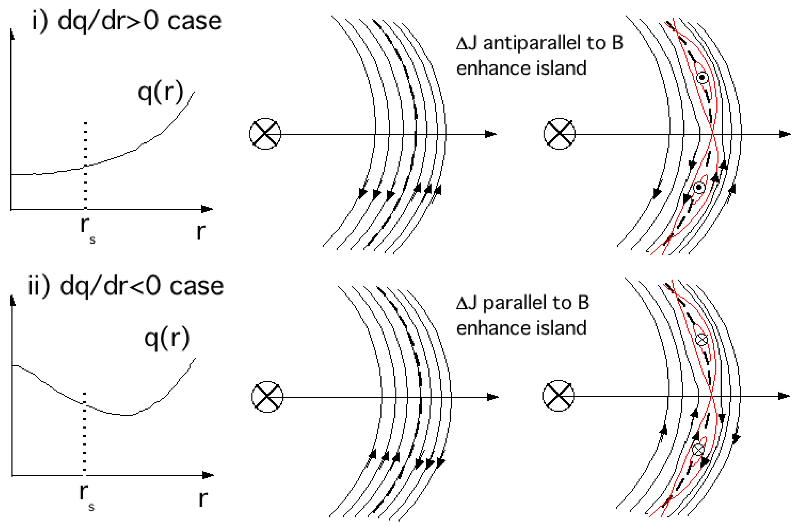
5.2. Tearing and Neoclassical Tearing Modes

In tokamaks, most unstable kink modes with poloidal mode number m = 1,2,3 can be stabilized if the safety factor at 95% flux surface q95 is above 3 (q95 > 3) which is the ITER standard operation condition. Operation of q(0) < 1 gives rise to the m = 1 internal kink instability. Stability of these linear ideal MHD modes can be analyzed using 2D Newcomb equation.
Finite resistivity in a high temperature plasma gives rise to resistive instabilities. This finite resistivity enables kink-like deformation with its resonant surface inside the plasma by changing the magnetic field topology at rational surface through magnetic reconnection to create magnetic island and is called “tearing instability”. This instability with poloidal and toroidal mode numbers m/n = 2/1, 3/1 3/2 is particularly important in a tokamak. The resistive instability with mode number m/n = 1/1 is somewhat different from others due to the breakdown of constant ψ approximation at the rational surface and is called resistive kink mode as cause of sawtooth oscillation through reconnection. When constant ψ approximation at resonant surface is valid, perturbed flux ψ = irBr/m (Br: perturbed radial magnetic field) is approximately governed by following diffusion equation:
ψ t = η μ 0 2 ψ r 2
This gives rise to the evolution of magnetic island width w as dw/dt = ηΔ’(w)/2μ0 [or more accurately dw/dt = 1.66η(Δ’(w) − αw)/μ0), where Δ’(w) = [dψ/dr(rs + w/2) − dψ/dr(rs − w/2)]/ψ(rs)]. As seen from Figure 25, the perturbed current inside the magnetic island is antiparallel to the equilibrium plasma current to form counter clockwise field lines around the island for the case of positive magnetic shear s > 0 (s = (r/q)dq/dr). The formation of magnetic islands reduces the pressure gradient and the reduction of the bootstrap current occurs and accelerates the growth of magnetic islands. This mode is called neoclassical tearing mode (NTM). On the other hand, the perturbed current is parallel to the equilibrium plasma current and reduction of the bootstrap current reduces the magnetic island for s < 0.
Figure 25. Relative magnetic field line flow inside and outside of resonant surface in equilibrium, the formation of magnetic island by the magnetic reconnection shown by red line for i) positive magnetic shear s = rdq/dr/q > 0 case and ii) negative magnetic shear s = rdq/dr/q < 0 case.
Energies 03 01741 g025

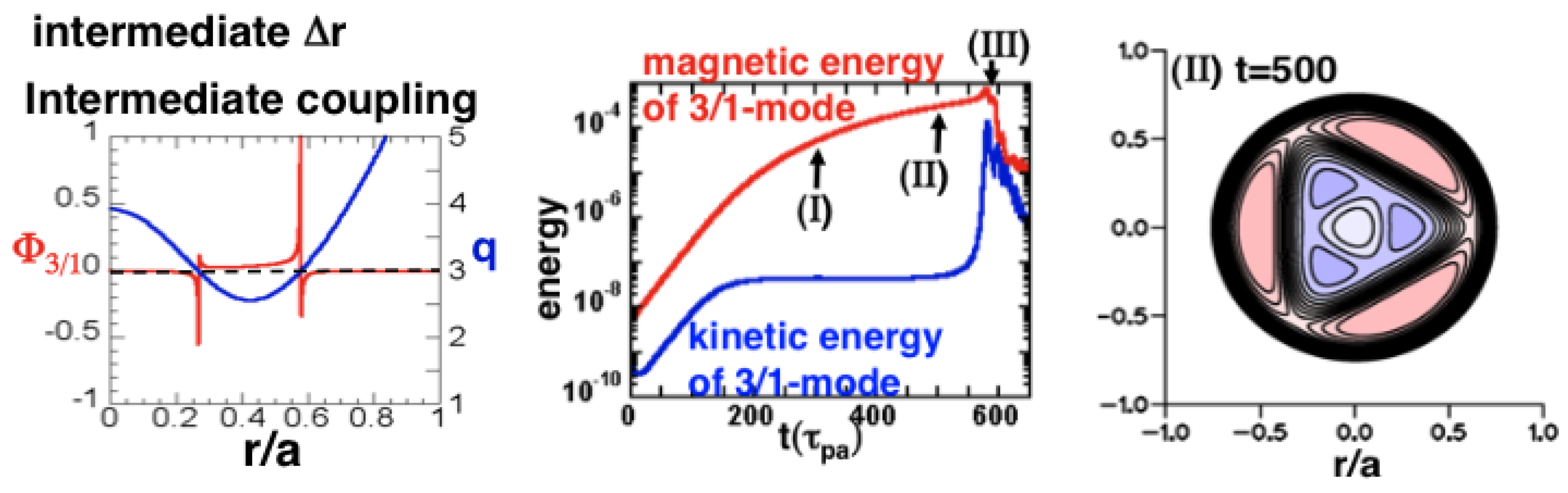
5.3. Double Tearing Modes in Negative Shear Plasma

Negative shear or reversed shear shown in Figure 26 (ii) is stable to NTM but is subject to double tearing mode (DTM) since there are two rational surfaces. DTM can grow explosively if mode coupling between two rational surfaces is strong. An explosive growth of DTM can occur after quiescent Rutherford regime by nonlinear destabilization of high m/n modes for intermediate separation of two rational surfaces [131]. If the separation between two rational surfaces is large enough, modes are decoupled and island will not grow explosively. Important implication for the plasma control is to pass through low m/n rational qmin as quick as possible under reduced pressure gradient and keep wider separation in quasi steady state [132].
Figure 26. DTM linear mode structure for intermediate separation of rational surfaces (left), time evolution of magnetic and kinetic energies in nonlinear DTM simulation (middle) and magnetic island before explosive growth (right) [131].
Energies 03 01741 g026

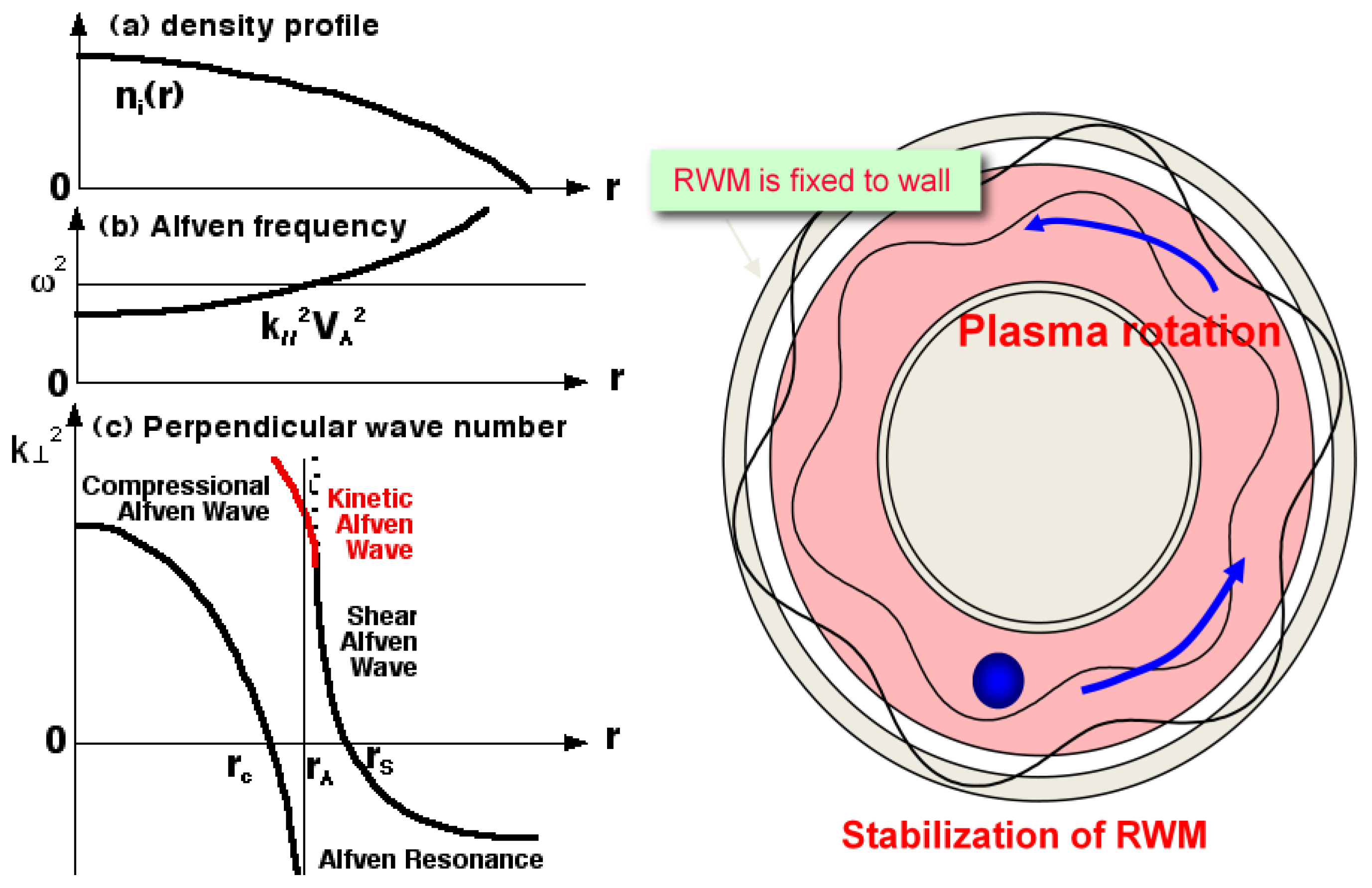
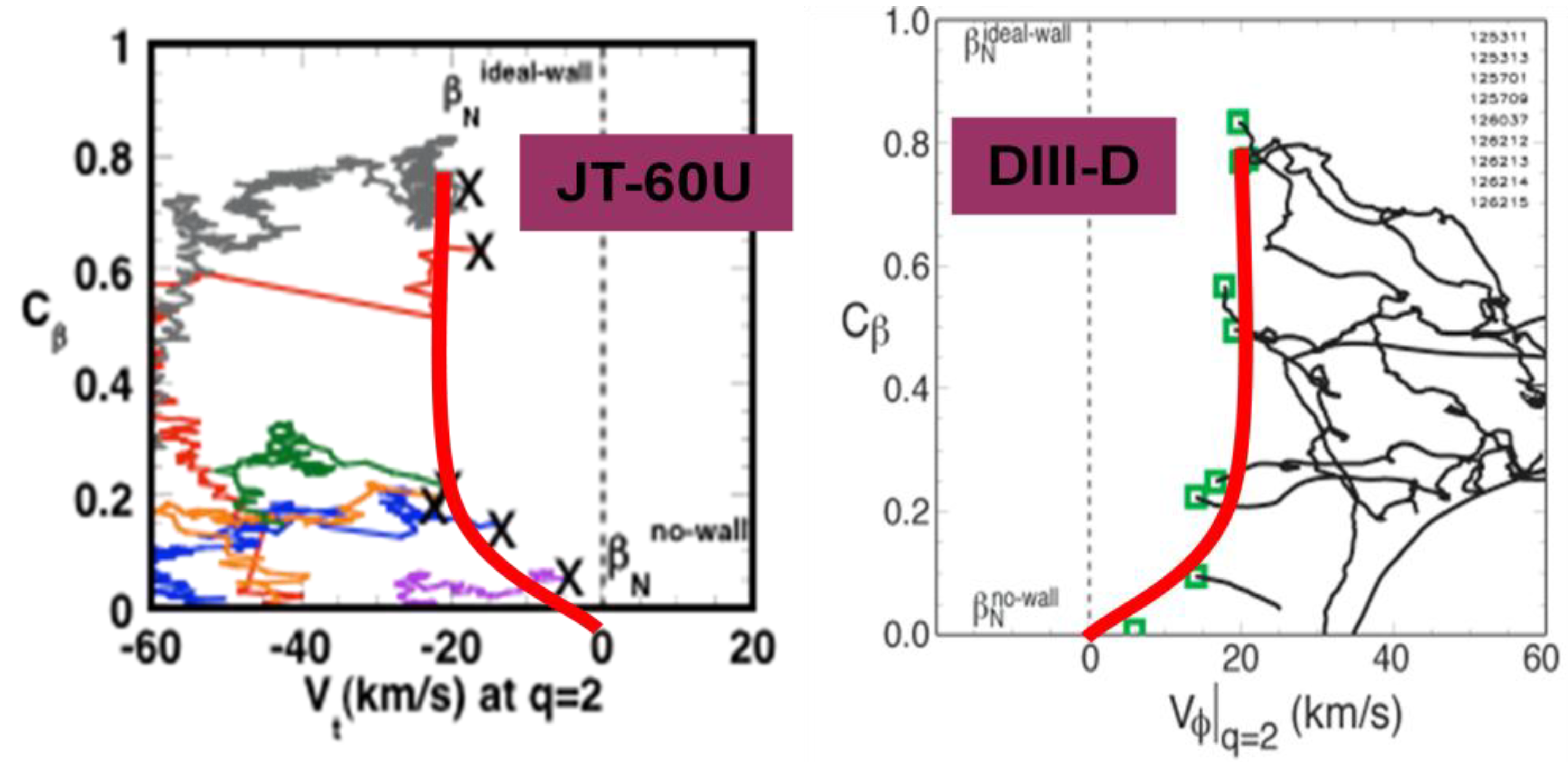
5.4. Resistive Wall Modes

When the SSTR concept was presented at the 1990 IAEA conference with q(0) > 2 for ballooning mode stability, this calls for Ramos’ idea on ideal MHD stability that the free boundary beta limit is inversely proportional to q(0) due to low m, n modes at this conference, later published in 1991 [133]. He proposed a modification to Troyon scaling as follows:
β t = β N q 0 I p a B t
This is true for free boundary modes, but the situation with a stabilizing wall is quite different. The MHD stability of SSTR for low m, n kink-ballooning modes are analyzed and found to be stable when q(0) > 2 with wall stabilization [78].
Figure 27. Schematic diagram of Alfven wave resonance and mode conversion to Kinetic Alfven Wave (KAW) indicating existence of shear Alfven wave continuum (left) [139] and schematic figure of plasma stability under resistive wall (right). The resistive wall mode (RWM) is fixed to the wall while plasma is moving in the toroidal direction. So in the moving frame, RWM is regarded as traveling wave by the plasma.
Energies 03 01741 g027
At that time, most people believed that wall stabilization may not work for realistic tokamak circumstances since a wall necessarily has finite resistance and penetration of the magnetic field will nullify wall stabilization. Even if plasma is rotating in the toroidal direction, it was believed that the mode [called resistive wall mode (RWM)] is attached to the wall and the mode will slip with respect to the plasma rotation [134,135].
It was unfortunate that it was not well recognized at that time that it was already shown shear Alfven wave has a continuous spectrum in the inhomogeneous plasma as shown in Figure 27 and RWM mode may damp by the phase mixing process or by the Landau damping through the mode conversion of shear Alfven wave to the kinetic Alfven wave, as already shown by Hasegawa and Chen in 1974–1976 [136,137,138,139]. We should also note that mode conversion to KAW was already observed experimentally in 1989 [140]. The same mechanism works for TAE modes called continuum damping [141,142], which was also confirmed experimentally in 1995 [143]. In 2007, both DIII-D [144] and JT-60U [145] showed that RWM is stabilized with small toroidal rotation close to the expectation by the continuous damping of Alfven wave, as shown in Figure 28.
Figure 28. Demonstration of stabilization of RWM by small toroidal plasma rotation in JT-60U (left) [145] and in DIII-D (right) [144].
Energies 03 01741 g028
Effect of wall stabilization in ideal MHD stability was studied by Manickam in 1994 for both positive and negative shear regimes, as shown in Figure 29 [146]. Beta limit is limited by n = 1 mode without wall stabilization and medium n for wall stabilized plasma. Changes in the beta limit between with and without wall stabilization is quite large for negative shear case. The reason for this is quite simple: wall stabilization is easy if the current is closer to the wall but such a surface current is unstable if wall is not effective.
One of practical issues of wall stabilization for tokamak system is the installation of an active feedback control coil, which is now actively discussed in ITER. Another important issue is the relative proximity of the resistive wall in the tokamak reactor [147]. Since the replaceable blanket should be replaced every few years, they must be segmented to reduce electromagnetic force and will not have good shell effect against kink like modes. So, a reactor will have rwall/a = 1.3 to 1.4. Hence, the integrated optimization of blanket and RWM stabilization is important.
Figure 29. Comparison of beta limit with and without wall stabilization for positive shear regime q(0)~1 (left) and negative shear regime (right) by Manickam [146].
Energies 03 01741 g029

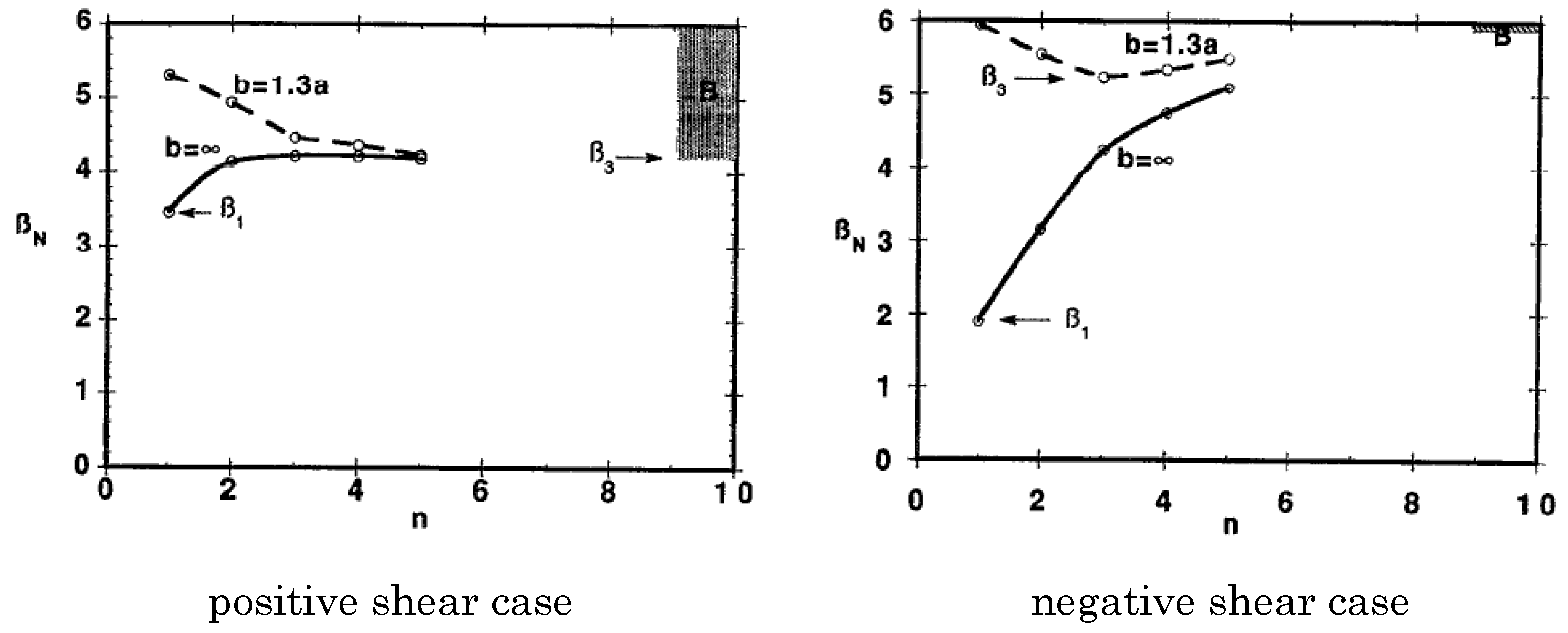
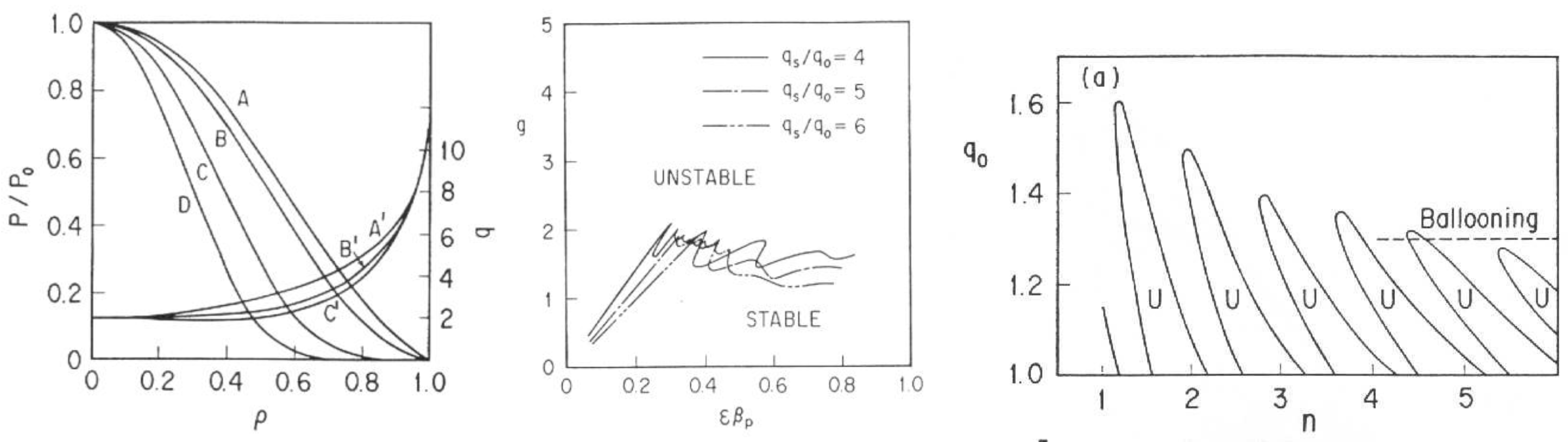
5.5. Ballooning and Peeling Modes
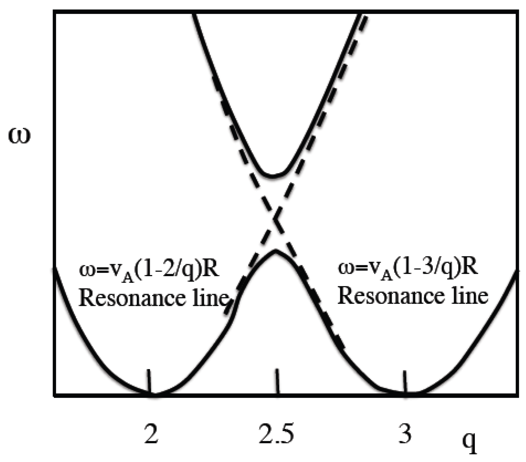
The stability of the ballooning mode is determined by the balance between the bending energy δWSA and the interchange energy δWIC. Ballooning mode has a unique structure with a double periodic condition in poloidal and toroidal directions and is given as summation of quasi-modes in covering space (−∞,∞) and is regarded as infinite radial overlapping of resonant modes.
The finite edge current can drive external modes localized near the plasma edge. This mode is called peeling mode. Peeling mode becomes most unstable when a rational surface is located just outside the plasma surface. This mode can be coupled to pressure driven ballooning mode and is thought to be a cause of ELM (Edge Localized Modes) in tokamaks.
One important attractive feature of a high βp regime is stable access to the second stability regime of ideal ballooning by increasing q(0) [148,149,150,151]. Second stability access near the plasma edge is possible with high edge current density, but the existence of peeling mode near the edge makes it complicated. This mode is destabilized by the edge current, especially edge bootstrap current by the steep pressure gradient.
Local confinement improvement in the edges and inside the plasma results in the edge transport barrier (ETB) (called H-mode) and internal transport barrier (ITB), respectively. These lead to increases of the local pressure gradient destabilizing ballooning mode through an increase in δWIC and peeling mode as a combination of δWIC and δWkI near the confinement barriers. These localized instabilities at ETB and ITB are called edge localized mode (ELM) and barrier localized mode (BLM) [152], respectively.
In the collisionless edge plasmas, a steep pressure gradient near the edge produces a large edge bootstrap current. This edge bootstrap current destabilizes the peeling mode and the radial extent of peeling mode becomes larger with the magnitude of thye edge bootstrap current. This situation is particularly crucial for power control of ELM energy loss in ITER and beyond.

5.6. Infernal Modes

If the magnetic shear is finite, radial coupling of various resonant MHD modes (m, m ± 1, m ± 2,--) becomes strong since radial separation between modes is small. However, if the magnetic shear is very low s = rdq/dr/q~0, radial mode separation becomes larger and radial mode coupling becomes weaker and standard ballooning mode theory base on dense radial mode coupling breaks down [153] (Hastie and Taylor derived the applicable conditions of ballooning mode theory as n >> (ψq’(ψ))−2 >> 1). Mode growth rate becomes oscillatory as a function of n (or toroidal wave number kz) treated as a continuous parameter. Under such circumstances, an intermediate integer n mode may become unstable even if lower n modes are stable. This low n internal pressure-drive mode was named “infernal mode” by Manickam [154] and is responsible for the βp collapses in JT-60U high βp regime.
Figure 30. From left, assumed pressure and q profiles for ideal MHD stability calculation (A’(li = 1.2), B’(li = 1), (C’:li = 0.8)), calculated stable-unstable boundaries of normalized beta g (= βN) for a relatively peaked pressure profile C, and infernal mode stability regime in (n, q0) space [94].
Energies 03 01741 g030
Ideal MHD stability of a high βp plasma was investigated by T. Ozeki to explain βp collapses as shown in Figure 30 [94]. A peaked pressure profile decreases the beta limit βN to low values (βN = 1.5 to 2) in a range of current profiles (li = 0.8 to 1.2), as observed in high performance high βp discharges [89]. In the case of high li~1.2 and peaked pressure profiles, beta limits observed as βp collapses are identified as internal kink modes, especially by the infernal mode in the low q(0) regime. With increasing q(0) (lowering li), infernal mode is stabilized because of the increase in the magnetic well depth [94].

5.7. Alfven Eigenmodes

There are two Alfven waves in a uniform plasma immersed in a static magnetic field. One is the shear Alfven wave (displacement vector ξ is perpendicular to B) and other is the compressional Alfven wave (ξ parallel to B). The shear Alfven wave at some location can have a resonance independent from neighboring field lines and the resonant condition (k→∞) can be expressed by ω = k//vA, where vA = B/(μ0nimi)1/2 is the Alfven velocity. Near the shear Alfven resonance, the shear Alfven wave is mode-converted to a kinetic Alfven wave and strong damping of the wave occurs as long as resonance exists in the plasma, as shown in Figure 31 (left), but for a frequency slightly lower than min (k//vA) (no shear Alfven resonance) in the plasma but cut-off still exists in the plasma, a shear Alfven wave can exist without strong damping and is called Global Alfven Eigenmodes (GAE).
In toroidal geometry where in-out inhomogeneity B~B0/(1 + εcosθ) exists, the Alfven resonance condition is given by a coupling of m (k//m = (n + m/q)/R) and m + 1 modes as:
| k / / m 2 ω 2 v A 2 ε ω 2 v A 2 ε ω 2 v A 2 k / / m + 1 2 ω 2 v A 2 | = 0
This gives a forbidden band of ω for Alfven wave resonance as shown in Figure 31. As we know, sin(mθ) + sin((m + 1)θ)=sin((m + 0.5)θ)cos(0.5θ), which implies periodicity after two circulation similar to Mobius band. The Mobius band is not orientable and there is no distinction between front and back surfaces. In this situation, it is difficult to have Alfven resonance, which is an explanation of the gap in the shear Alfven resonance. Although resonance does not occur, shear Alfven mode can propagate for a frequency range in the gap as point (or discrete) spectrum and can be destabilized by the interaction with fast ions as shown by Cheng [155,156].
Figure 31. Alfven gap frequency structure due to toroidal mode coupling of m = 1 and m = 2 modes in (q, ω) plane.
Energies 03 01741 g031
This TAE was first observed in neutral beam heated plasma by Wong [157]. A review of Alfven Eigenmodes was given by Wong [158]. Alfven eigenmodes due to a particles in ITER are an important control issue. In JT-60U, TAE are observed during ICRF heating [159,160], and new Alfven Eigenmode Non-circular Alfven Eigenmode was observed [161]. TAE modes including chirping modes and reversed shear Alven eigenmodes are also observed during N-NBI heating [162,163].

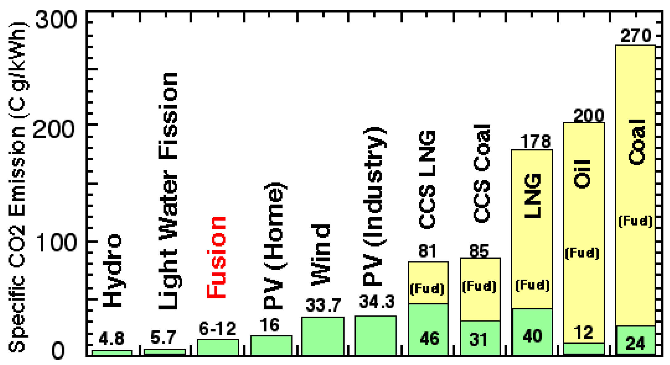
6. Role of Fusion Energy in the 21st Century [3]

To prevent global warming, a low carbon society free from fossil energy must be achieved during the 21st century. Although attention has been paid to electricity and hydrogen power as clean energies, low CO2 emission energy sources must be used to create electricity and hydrogen. CO2 emission per electric power kwh is an important figure of merit and is called specific CO2 emission. As shown in Figure 32, fusion is one of energy sources with low specific CO2 emission next to hydro and light‑water reactor.
Figure 32. Specific CO2 emission of fired (coal, oil, natural gas), renewables (solar, wind), fission and fusion plants. Green and yellow indicate CO2 emission by construction and fuel burn, respectively. Abbreviations are Carbon Capture and Sequestration (CCS) and Photo Voltaic (PV).
Energies 03 01741 g032
In light water reactors and fast reactors, iodine 131 (131I) produced by the reaction tend to accumulate in certain organs of human body, and the concentration limit in the air (tolerance) is set to very low levels. The hazard potential of 131I in a 1 GW fission power station is about 1,000 times larger than that of tritium (T) in a 1 GW fusion power station (Figure 33). Therefore, fusion energy has favorable characteristics in terms of radiation hazards.
Figure 33. Comparison of fired, fission and fusion on radiation hazard potential and specific CO2 emission.
Energies 03 01741 g033
Realization of a low carbon society by suppressing the use of fossil fuels is necessary to prevent global warming and emissions of greenhouse gases like carbon dioxide and methane. According to the 2100 nuclear vision proposed by the office of Strategy Research, Japan Atomic Energy Agency [164], an option to utilize previous R&D results and atomic energy technologies under development to reduce national CO2 emission to 10% of present value while maintaining stable energy supply in 2100 as shown in Figure 34. In that scenario, use of fossil energy currently sharing 85% of primary energy is reduced to 30% by the end of this century and the other 70% will be shared by non-fossil energy with a dominant contribution from Atomic Energy.
Figure 34. CO2 reduction scenario (left) and Electricity supply scenario from various sources (right) in Atomic Energy vision 2100 [164].
Energies 03 01741 g034
In this scenario, the use of electricity and hydrogen is promoted as an energy source. Significant reduction in energy consumption is realized by improved energy efficiency through the expanded use of electric vehicles and fuel cell vehicles by way of hybrid vehicles in the transport sector. Coal and oil use in industrial sector is eliminated by substituting coke as a reducing agent in the steel industry and naphtha in the chemical industry with hydrogen. Energy use in civilian areas may become electric except fpr solar heat.
In this way, 60% of the final energy demand in the year 2100 becomes electricity. It is difficult to respond to such a huge power demand with only renewable energy and a large-scale stable supply from Atomic Energy is most promising. In this vision, it is assumed that ~30 fusion plants will be operational in Japan by the end of this century assuming the scientific and technical feasibility of fusion energy is demonstrated in ITER and the construction and operation of DEMO progresses in a timely fashion to start construction of the first commercial fusion plants in the 2050s. It should be noted that it is possible that fusion energy will not be on the energy market by the end of 21st century if fusion R&D does not go well or its economic efficiency and reliability of operation are not good enough.
The tokamak system adopted in ITER shows the best performance in high temperature plasma confinement. The operation of a tokamak stops when an inductive electric field can’t be supplied since the confinement field is created by the inductive plasma current. As a power generation device it becomes pulsed. As a method to overcome this drawback and to produce energy continuously, the use of bootstrap current is considered. Since 80% of the plasma current is shed by the bootstrap current in JT-60 (Figure 21), a steady-state tokamak reactor (SSTR) is designed as a practical way in cooperation with industries [78].
To achieve a continuous operation using the bootstrap current, the majority of the plasma current has to be driven by the bootstrap current and rest by a beam or in some other way, as shown in Figure 35. The heat including the generation inside the blanket is removed and converted to electricity in a steam turbine and a fraction is used as recirculating power for beam generation and other plant needs. Achievement of continuous operation with Q > 5 given in the ITER technical objectives is important. In this case, about half of the plasma current should be driven by the bootstrap current while the rest should be driven by the beam-driven current.
Figure 35. Principle to achieve high net generated power by achieving efficient continuous operation using bootstrap current.
Energies 03 01741 g035

7. Concluding Remarks

Fusion research has progressed significantly during the 50 years elapsed since its inception in 1958, especially thanks to tokamak research. In this review, a brief introduction of fusion reaction, topology of magnetic confinement and hidden symmetry in force equilibrium is provided leading to the importance of the apparent geometrical symmetry of the tokamak. This symmetry in a tokamak is created by the toroidal plasma current, leading to the question of continuous operation. The bootstrap current driven by the plasma itself provided an opportunity for continuous operation and the concept of a steady state tokamak reactor was formed in 1990, clarifying the necessary plasma regime for the operation of a steady-state tokamak reactor. In this review, the theoretical foundation of the generalized Ohm’s law and its experimental confirmation, creation of advanced operational regimes for steady state tokamaks, and progress in our understanding of MHD stability issues of a steady-state tokamak are highlighted. Finally, a view of fusion energy utilization in 21st century is introduced by assuming smooth advances in ITER and DEMO development. This review is a partial review of research towards realization of a steady state tokamak fusion system with emphasis on the principles, physics of plasma currents in tokamaks and a description of important MHDs, and the role of fusion in the 21st century. A more comprehensive physics review will be given elsewhere.

Acknowledgements

The author acknowledges the former executive director of JAERI, Hiroshi Kishimoto (past) for his leadership and excellent vision in directing advanced tokamak research in JT-60U.

References

  1. Kikuchi, M. Editorial of Special Issue: Fifty years of fusion research and the road to fusion energy. Nucl. Fusion 2010, 1, 010202. [Google Scholar]
  2. Kikuchi, M.; Inoue, N. Role of Fusion Energy for the 21st Century Energy Market and Development Strategy with International Thermonuclear Experimental Reactor. In Proceedings of the 18th World Energy Congress, Buenos Aires, Argentina, 21–25 October, 2001.
  3. Kikuchi, M. Physics and Fusion; Kyoto University Press: Kyoto, Japan, 2009; in Japanese. [Google Scholar]
  4. Ikeda, K. ITER on the road to fusion energy. Nucl. Fusion 2010, 50, 014002. [Google Scholar] [CrossRef]
  5. Kikuchi, M. Steady-state tokamak reactor based on the bootstrap current. Nucl. Fusion 1990, 30, 265–276. [Google Scholar] [CrossRef]
  6. Seki, Y.; Kikuchi, M.; Ando, T.; Ohara, Y.; Nishio, S.; Seki, M.; Takizuka, T.; Tani, K.; Ozeki, T.; Koizumi, K.; et al. The Steady State Tokamak Reactor. In Proceedings of the 13th International Conference on Plasma Physics and Controlled Nuclear Fusion Research, Washington, DC, USA, 1–6 October 1990.
  7. Kikuchi, M.; Seki, Y.; Oikawa, A.; Ando, T.; Ohara, Y.; Nishio, S.; Seki, M.; Takizuka, T.; Tani, K.; Ozeki, T.; et al. Conceptual design of the steady-state tokamak reactor (SSTR). Fusion Eng. Des. 1991, 18, 195–202. [Google Scholar] [CrossRef]
  8. Kishimoto, H.P.; Ishida, S.; Kikuchi, M.; Ninomiya, H. Advanced tokamak research on JT-60. Nucl. Fusion 2005, 45, 986–1023. [Google Scholar] [CrossRef]
  9. Kitsunezaki, A.; Shimizu, M.; Ninomiya, H.; Kuriyama, M. Special Issue on JT-60. Fusion Sci. Technol. 2002, 42, 179–539. [Google Scholar]
  10. Yoshikawa, M. JT-60 Team. Recent experiments in JT-60. In Proceedings of 11th International Conference on Plasma Physics and Controlled Nuclear, Kyoto, Japan, 13–20 November 1986.
  11. Kishimoto, H. JT-60 team. Recent progress in JT-60 experiments. In Proceedings of 12th International Conference on Plasma Physics and Controlled Nuclear, Nice, France, 12–19 October 1988.
  12. Nagami, M. JT-60 team. Recent experiments in JT-60. In Proceedings of 13th International Conference on Plasma Physics and Controlled Nuclear, Washington, DC, USA, 1–6 October 1990.
  13. Shimada, M. JT-60 team. JT-60U high power heating experiments. In Proceedings of 14th International Conference on Plasma Physics and Controlled Nuclear, Germany, 30 September–7 October 1992.
  14. Kikuchi, M. JT-60 team. Recent JT-60U results towards steady-state operation of tokamaks. In Proceedings of 15th International Conference on Plasma Physics and Controlled Nuclear, Seville, Spain, September 26–October 1, 1994.
  15. Ushigusa, K. JT-60 Team. Steady state operation research in JT-60U. In Proceedings of 16th International Conference on Plasma Physics and Controlled Nuclear, Montreal, Canada, 7–11 October 1996.
  16. Ishida, S. JT-60 Team. JT-60U high performance regime. Nucl. Fusion 1999, 39, 1211. [Google Scholar] [CrossRef]
  17. Kamada, Y. JT-60 Team. Extended JT-60U plasma regimes for high integrated performance. Nucl. Fusion 2001, 41, 1311. [Google Scholar] [CrossRef]
  18. Fujita, T. JT-60 Team. Overview of JT-60U results leading to high integrated performance in reactor-relevant regime. Nucl. Fusion 2003, 43, 1527. [Google Scholar] [CrossRef]
  19. Ide, S. JT-60 Team. Overview of JT-60U progress towards steady-state advanced tokamak. Nucl. Fusion 2005, 45, S48. [Google Scholar] [CrossRef]
  20. Takenaga, H. JT-60 Team. Overview of JT-60U results for the development of a steady-state advanced tokamak scenario. Nucl. Fusion 2007, 47, S563. [Google Scholar] [CrossRef]
  21. Oyama, N. JT-60 Team. Overview of JT-60U results towards the establishment of advanced tokamak operation. Nucl. Fusion 2009, 49, 104007. [Google Scholar] [CrossRef]
  22. Ninomiya, H. JT-60 Team. JT-60U latest results and future prospects. Phys. Fluids 1992, B4, 2070. [Google Scholar]
  23. Hosogane, N. JT-60 Team. Confinement and divertor studies in Japan tokamak JT-60U. Phys. Fluids 1993, B5, 2412. [Google Scholar] [CrossRef]
  24. Kondoh, T. High performance and current drive experiments in the JAERI tokamak-60 upgrade. Phys. Plasmas 1994, 1, 1489. [Google Scholar] [CrossRef]
  25. Fukuda, T. JT-60 Team. Steady-state improved confinement studies in the JT-60U tokamak. Phys. Plasmas 1995, 2, 2249. [Google Scholar] [CrossRef]
  26. Kimura, H. JT-60 Team. Recent results from high performance and steady-state researches in the Japan Atomic Energy Research Institute Tokamak-60 Upgrade. Phys. Plasmas 1996, 3, 1943. [Google Scholar] [CrossRef]
  27. Koide, Y. Progress in confinement and stability with plasma shape and profile control for steady-state operation in the Japan Atomic Energy Research Institute Tokamak-60 upgrade. Phys. Plasmas 1997, 4, 1623. [Google Scholar] [CrossRef]
  28. Shirai, H. JT-60 Team. Recent experimental and analytic progress in the Japan Atomic Energy Research Institute Tokamak-60 upgrade with W-shaped divertor configuration. Phys. Plasmas 1998, 5, 1712. [Google Scholar] [CrossRef]
  29. Kusama, Y. Recent progress in high performance and steady-state experiments on the Japan Atomic Energy Research Institute tokamak-60 upgrade with W-shaped divertor. Phys. Plasmas 1999, 6, 1935. [Google Scholar] [CrossRef]
  30. Ide, S. Latest progress in steady state plasma research on the Japan Atomic Energy Research Institute Tokamak-60 Upgrade. Phys. Plasmas 2000, 7, 1927. [Google Scholar] [CrossRef]
  31. Takenaga, H. Improved particle control for high integrated plasma performance in Japan Atomic Energy Research Institute Tokamk-60 Upgrade. Phys. Plasmas 2001, 8, 2217. [Google Scholar] [CrossRef]
  32. Kubo, H. Extension of integrated high performance regimes with impurity and deuterium particle control in Japan Atomic Energy Research Institute Tokamak-60 Upgrade (JT-60U). Phys. Plasmas 2002, 9, 2127. [Google Scholar] [CrossRef]
  33. Miura, Y. Study of improved confinement modes with edge and/or internal transport barriers on the Japan Atomic Energy Research Institute Tokamak-60 Upgrade (JT-60U). Phys. Plasmas 2003, 10, 1809. [Google Scholar] [CrossRef]
  34. Ishida, S. JT-60 Team. High-beta steady-state research and future directions on the Japan Atomic Energy Research Institute Tokamak-60 Upgrade and the Japan Atomic Energy Research Institute Fusion Torus-2 Modified. Phys. Plasmas 2004, 11, 2532. [Google Scholar] [CrossRef]
  35. Isayama, A. Steady-state sustainment of high-β plasmas through stability control in Japan Atomic Energy Research Institute tokamak-60 upgrade. Phys. Plasmas 2005, 12, 056117. [Google Scholar] [CrossRef]
  36. Fujita, T. Advanced tokamak research on long time scales in JT-60U upgrade. Phys. Plasma 2006, 13, 056112. [Google Scholar] [CrossRef]
  37. Ozeki, T. High-beta steady-state research with integrated modeling in the JT-60 upgrade. Phys. Plasmas 2007, 14, 056114. [Google Scholar] [CrossRef]
  38. Hayashi, N. Advanced tokamak research with integrated modeling in JT-60 Upgrade. Phys. Plasmas 2010, 17, 056112. [Google Scholar] [CrossRef]
  39. Kikuchi, M. Summary of steady-state research during 23 years of JT-60 tokamak experiments. Bull. Am. Physical Soc. 2009, NO4, 1. [Google Scholar]
  40. Yoshikawa, M. Initial experiments in JT-60. Plasma Phys. Control. Fusion 1986, 28, 165. [Google Scholar] [CrossRef]
  41. Tamura, S. Status of JT-60 experiments. Plasma Phys. Control. Fusion 1986, 28, 1377. [Google Scholar] [CrossRef]
  42. Yoshino, R. High power heating and current drive in JT-60. Plasma Phys. Control Fusion 1987, 29, 1377. [Google Scholar] [CrossRef]
  43. Akiba, M. High power heating results on JT-60. Plasma Phys. Control Fusion 1988, 30, 1405. [Google Scholar] [CrossRef]
  44. Nagami, M. Recent results in JT-60 experiments. Plasma Phys. Control Fusion 1989, 31, 1597. [Google Scholar] [CrossRef]
  45. Ushigusa, K. Recent results of LH experiments on the JT-60 tokamak. Plasma Phys. Control Fusion 1990, 32, 853. [Google Scholar] [CrossRef]
  46. Naito, O. Steady State Plasma Performance on JT-60U. Plasma Phys. Control. Fusion 1993, 35, B215–B222. [Google Scholar] [CrossRef]
  47. Mori, M. Latest results from JT-60U. Plasma Phys. Control. Fusion 1994, 36, B181–B191. [Google Scholar] [CrossRef]
  48. Itami, K. Improved Confinement of JT-60U plasmas. Plasma Phys. Control. Fusion 1995, 37, A255–A265. [Google Scholar] [CrossRef]
  49. Neyatani, Y. Improved confinement with plasma profile and shape controls in JT-60U. Plasma Phys. Control. Fusion 1996, 38, A181–A191. [Google Scholar] [CrossRef]
  50. Fujita, T. High-performance experiments towards steady-state operation in JT-60U. Plasma Phys. Control. Fusion 1997, 39, B75–B90. [Google Scholar] [CrossRef]
  51. Tobita, K. Latest plasma performance and experiments on JT-60U. Plasma Phys. Control Fusion 1999, 41, A333–A343. [Google Scholar] [CrossRef]
  52. Kamada, Y. Extension of the JT-60U plasma regimes toward the next-step experimental reactor. Plasma Phys. Control Fusion 1999, 41, B77–B92. [Google Scholar] [CrossRef]
  53. Kikuchi, M. Advanced Scenarios in JT-60U—Integration towards a reactor relevant regime. Plasma Phys. Control Fusion 2001, 43, 217. [Google Scholar] [CrossRef]
  54. Fukuda, T. Development of high-performance discharges with transport barriers in JT-60U. Plasma Phys. Control Fusion 2002, 44, B39. [Google Scholar] [CrossRef]
  55. Kikuchi, M. Plasma Physics found in JT-60 Tokamak over the Last 20 years. AIP Conf. Ser. 2009, 1150, 161–167. [Google Scholar]
  56. Mott, N.F.; Massey, H.S.W. The Theory of Atomic Collisions, 3rd Ed. ed; Oxford Clarendon Press: Oxford, UK, 1965. [Google Scholar]
  57. Duane, B.H. Fusion Cross-Section Theory; Technical Report for Brookhaven National Laboratory: Upton, NY, USA, January 1972; BNWL-1685. [Google Scholar]
  58. Li, X.Z.; Wei, Q.M.; Liu, B. A new simple formula for fusion cross-sections of light nuclei. Nucl. Fusion 2008, 48, 125003. [Google Scholar] [CrossRef]
  59. Poincare, H. Sur les courbes definies par les equations differentielles. Journal de Mathematiques pures et appliqués 1885, 4, 167–244. [Google Scholar]
  60. Kruskal, M.D.; Krusrud, R.M. Equilibrium of a Magnetically confined Plasma in a Toroid. Phys. Fluids 1958, 1, 265–274. [Google Scholar] [CrossRef]
  61. Hirshman, S.P.; Whitson, J.C. Steepest-decent moment-method for three dimensional magneto hydrodynamic equilibria. Phys. Fluids 1983, 26, 3553–3568. [Google Scholar] [CrossRef]
  62. Lao, L.L.; Hirshman, S.P.; Wieland, R.M. Variational moment solutions to the Grad-Shafranov equation. Phys. Fluids 1981, 24, 1431–1441. [Google Scholar] [CrossRef]
  63. Grad, H.; Rubin, H. Hydromagnetic Equilibria and Force-Free Field. In Proceedings of the 2nd UN International Conference on Peaceful Use of Atomic Energy, Geneva, Switzerland, 1–13 September 1958.
  64. Shafranov, V.D. Plasma Equilibrium in a Magnetic Field; Leontovich, M.A., Ed.; Consultants Bureau: New York, NY, USA, 1966; Volume II. [Google Scholar]
  65. McGuire, K.M.; Barnes, C.W.; Batha, S.H.; Beer, M.A.; Bell, M.G.; Bell, R.E.; Belov, A.; Berk, H.L.; Bernabei, S.; Bitter, M.; et al. Physics of High Performance Deuterium-Tritium Plasmas in TFTR. In Proceedings of the 16th International Conference on Plasma Physics and Controlled Nuclear Fusion Research, Montreal, Canada, 7–11 October 1996.
  66. Watkins, M.L. Physics of high performance JET plasmas in DT. Nucl. Fusion 1999, 39, 1227–1244. [Google Scholar] [CrossRef]
  67. Conn, R.W.; Kulcinski, G.L.; Maynard, C.W.; Aronstein, R.; Boom, R.W.; Bowles, A.; Clemmer, R.G.; Davis, J.; Emmert, G.A.; Ghose, S.; et al. A High-performance non-circular tokamak power reactor design study—UWMAK-III. In Proceedings of the 16th International Conference on Plasma Physics and Controlled Nuclear Fusion Research, Montreal, Canada, 7–11 October 1996.
  68. Fisch, N.J. Confining a Tokamak Plasma with rf-Driven Currents. Phys. Rev. Lett. 1978, 41, 873. [Google Scholar] [CrossRef]
  69. Yamamoto, T.; Imai, T.; Shimada, M.; Suzuki, N.; Maeno, M.; Konoshima, S.; Fujii, T.; Uehara, K.; Nagashima, T.; Funahashi, A.; et al. Experimental Observation of the rf-Driven Current by the Lower-Hybrid Wave in a Tokamak. Phys. Rev. Lett. 1980, 45, 716–719. [Google Scholar] [CrossRef]
  70. Baker, C.C.; Abdou, M.A.; Arons, R.M.; Bolon, A.E.; Boley, C.D.; Brooks, J.N.; Clemmer, R.G.; Dennis, C.B.; Ehst, D.A.; Evans, K.E., Jr.; et al. STARFIRE—A Commercial Tokamak Fusion Power Plant Study; Technical Report for Argonne National Laboratory: Argonne, IL, USA, September 1980; No. ANL/FPP-80-1. [Google Scholar]
  71. Bickerton, R.J.; Connor, J.W.; Taylor, J.B. Diffusion driven plasma currents and bootstrap tokamak. Nature Phys. Sci. 1971, 229, 110. [Google Scholar] [CrossRef]
  72. Galeev, A.A.; Sagdeev, R.Z. The theory of plasma confinement in a tokamak at high temperature. Nucl. Fusion suppl. 1972, 12, 45–51. [Google Scholar] [CrossRef]
  73. Kikuchi, M.; Azumi, M.; Tsuji, S.; Tani, K.; Kubo, H. Bootstrap current during perpendicular neutral injection in JT-60. Nucl. Fusion 1990, 30, 343–355. [Google Scholar] [CrossRef]
  74. Conn, R.W.; Najmabadi, F. ARIES-I, A steady-state, first-stability tokamak reactor with enhanced safety and environmental features. In Proceedings of 13th International Conference on Plasma Physics and Controlled Nuclear, Washington, DC, USA, 1–6 October 1990.
  75. Kikuchi, M.; Seki, Y.; Nakagawa, K. The Advanced SSTR. Fus. Eng. Design 2000, 48, 265–270. [Google Scholar] [CrossRef]
  76. Najmabadi, F. Overview of ARIES-RS tokamak fusion power plant. Fus. Eng. Design 1998, 41, 365. [Google Scholar] [CrossRef]
  77. Okano, K.; Asaoka, Y.; Hiwatari, R.; Inoue, N.; Murakami, Y.; Ogawa, Y.; Tokimatsu, K.; Tomabechi, K.; Yamamoro, T.; Yoshida, T. Study of a compact reversed shear tokamak reactor. Fusion Eng. Des. 1998, 41, 511–517. [Google Scholar] [CrossRef]
  78. Fusion Reactor System Laboratory. Concept Study of the Steady State Tokamak Reactor (SSTR); Technical Report for Japan Atomic Energy Research Institute: Ibaraki, Japan, April 1991; JAERI-M Report-91-081. [Google Scholar]
  79. Nishio, S.; Ando, T.; Ohara, Y.; Mori, S.; Mizoguchi, T.; Kikuchi, M.; Oikawa, A.; Seki, Y. Engineering aspects of a steady state tokamak reactor (SSTR). Fusion Eng. Des. 1991, 15, 121–135. [Google Scholar] [CrossRef]
  80. Kikuchi, M.; Conn, R.W.; Najimabadi, F.; Seki, Y. Recent directions in plasma physics and its impact on tokamak magnetic fusion design. Fusion Eng. Des. 1991, 16, 253–270. [Google Scholar] [CrossRef]
  81. Troyon, F.; Gruber, R.; Sauremann, H.; Semenzato, S.; Succi, S. MHD-Limits to Plasma Confinement. Plasma Phys. Control Fusion 1984, 26, 209–215. [Google Scholar] [CrossRef]
  82. Stambaugh, R.; Moore, R.W.; Bernard, L.C.; Kellman, A.G.; Strait, E.J.; Lao, L.; Overskei, D.O.; Angel, T.; Armentrout, C.J.; Baur, J.F.; et al. Tests of Beta Limits as a Function of Plasma Shape in Doublet III. In Proceedings of the 10th International Conference on Plasma Physics and Controlled Nuclear Fusion Research, London, UK, 12–19 September 1984.
  83. Cordey, J.G.; Challis, C.D.; Stubberfield, P.M. Bootstrap current theory and experimental evidence. Plasma Phys. Control Fusion 1988, 30, 1625–1635. [Google Scholar] [CrossRef]
  84. Ferron, J.R.; Chu, M.S.; Helton, F.J.; Howl, W.; Kellman, A.G.; Lao, L.L.; Lazarus, E.A.; Lee, J.K.; Osborne, T.H.; Strait, E.J.; et al. High-beta discharges in the DIII-D tokamak. Phys. Fluids 1990, B2, 1280–1286. [Google Scholar] [CrossRef]
  85. Cheng, C.Z.; Furth, H.P.; Boozer, A.H. MHD stable regime of the Tokamak. Plasma Phys. Control Fusion 1988, 29, 351–366. [Google Scholar] [CrossRef]
  86. Kamada, Y.; Ushigusa, K.; Naito, O.; Neyatani, Y.; Ozeki, T.; Tobita, K.; Ishida, S.; Yoshino, R.; Kikuchi, M.; Mori, M.; Ninomiya, H. Non-inductively current driven H mode with high βN and high βp values in JT-60U. Nucl. Fusion 1994, 34, 1605–1618. [Google Scholar] [CrossRef]
  87. Ishida, S.; Kikuchi, M.; Hirayama, T.; Koide, Y.; Ozeki, T.; Tsuji, S.; Naito, O.; Shirai, H.; Nagami, M.; Azumi, M. High poloidal beta experiments with a hot ion enhanced confinement regime in the JT-60 tokamak. In Proceedings of 13th International Conference on Plasma Physics and Controlled Nuclear, Washington, DC, USA, 1–6 October 1990.
  88. Ishida, S.; Koide, Y.; Ozeki, T.; Kikuchi, M.; Tsuji, S.; Shirai, H.; Naito, O.; Azumi, M. Observation of a Fast Beta Collapse during High Poloidal-Beta Discharges in JT-60. Phys. Rev. Lett. 1992, 68, 1531–1534. [Google Scholar] [CrossRef] [PubMed]
  89. Ishida, S.; Matsuoka, M.; Kikuchi, M.; Tsuji, S.; Nishitani, T.; Koide, Y.; Ozeki, T.; Fujita, T.; Nakamura, H.; Hosogane, N.; et al. Enhanced confinement of high bootstrap current discharges in JT-60U. In Proceedings of 14th International Conference on Plasma Physics and Controlled Nuclear, Germany, 30 September–7 October 1992.
  90. Hawryluk, R.J.; Arunasalam, V.; Bell, M.G.; Bitter, M.; Blanchard, W.R.; Bretz, N.L.; Budney, R.; Bush, C.E.; Callen, J.D.; Cohen, S.A.; et al. TFTR plasma regimes. In Proceedings of 11th International Conference on Plasma Physics and Controlled Nuclear, Kyoto, Japan, 13–20 November 1986.
  91. Park, H.K.; Bell, M.G.; Yamada, M.; McGuire, K.M.; Sabbagh, S.A.; Budney, R.V.; Wieland, R.M.; the TFTR team; Ishida, S.; Nishitani, T.; Kawano, Y.; Kamada, Y.; Fujita, T.; Mori, M.; Koide, Y.; Shirai, H.; Kikuchi, M. Proceedings of 15th International Conference on Plasma Physics and Controlled Nuclear, Seville, Spain, 26 September–1 October, 1994.
  92. Ozeki, T.; Azumi, M.; Tsunematsu, T.; Tani, K.; Yagi, M.; Tokuda, S. Profile control for a stable high βp tokamak with a large bootstrap current. In Proceedings of 14th International Conference on Plasma Physics and Controlled Nuclear, Germany, 30 September–7 October 1992.
  93. Kessel, C.; Manickam, J.; Rewoldt, G.; Tang, W.M. Improved plasma performance in tokamaks with negative magnetic shear. Phys. Rev. Lett. 1994, 72, 1212–1215. [Google Scholar] [CrossRef] [PubMed]
  94. Ozeki, T.; Azumi, M.; Kamada, Y.; Ishida, S.; Neyatani, Y.; Tokuda, S. Ideal MHD stability of high βp plasmas and βp collapse in JT-60U. Nucl. Fusion 1995, 35, 861–871. [Google Scholar] [CrossRef]
  95. Levinton, F.M.; Zarnstorff, M.C.; Batha, S.H.; Bell, M.; Bell, R.E.; Budny, R.V.; Bush, C.; Chang, Z.; Fredrickson, E.; Janos, A.; et al. Improved confinement with reversed magnetic shear in TFTR. Phys. Rev. Lett. 1995, 75, 4417–4420. [Google Scholar] [CrossRef]
  96. Strait, E.J.; Lao, L.L.; Mauel, M.E.; Rice, B.W.; Taylor, T.S.; Burrel, K.H.; Chu, M.S.; Lazarus, E.A.; Osborne, T.H.; Thompson, S.J.; Turnbull, A.D. Enhanced confinement and stability in DIII-D discharges with reversed magnetic shear. Phys. Rev. Lett. 1995, 75, 4421–4424. [Google Scholar] [CrossRef] [PubMed]
  97. Fujita, T.; Ide, S.; Shirai, H.; Kikuchi, M.; Naito, O.; Koide, Y.; Takeji, S.; Kubo, H.; Ishida, S. Internal transport barrier for electrons in JT-60U reversed shear discharges. Phys. Rev. Lett. 1997, 78, 2377–2380. [Google Scholar] [CrossRef]
  98. Fujita, T.; Ide, S.; Kimura, H.; Koide, Y.; Oikawa, T.; Takeji, S.; Shirai, H.; Ozeki, T.; Kamada, Y.; Ishida, S. Enhanced core confinement in JT-60U reversed shear discharges. In Proceedings of 16th International Conference on Plasma Physics and Controlled Nuclear, Montreal, Canada, 7–11 October 1996.
  99. Fujita, T. High-performance experiments towards steady-state operation in JT-60U. Plasma Phys. Control Fusion 1997, 39, B75–B90. [Google Scholar] [CrossRef]
  100. Fujita, T.; Oikawa, T.; Suzuki, T.; Ide, S.; Sakamoto, Y.; Koide, Y.; Hatae, T.; Naito, O.; Isayama, A.; Hayashi, N.; Shirai, H. Plasma Equilibrium and Confinement in a Tokamak with Nearly Zero Central Current Density in JT-60U. Phys. Rev. Lett. 2001, 87, 245001. [Google Scholar] [CrossRef] [PubMed]
  101. Hawkes, N.C.; Stratton, B.C.; Tala, T.; Challis, C.D.; Conway, G.; DeAngelis, R.; Giroud, C.; Hobirk, J.; Joffrin, E.; Lomas, P.; et al. Observation of Zero Current Density in the Core of JET Discharges with Lower Hybrid Heating and Current Drive. Phys. Rev. Lett. 2001, 87, 115001. [Google Scholar] [CrossRef] [PubMed]
  102. Kikuchi, M. Prospects of a Stationary Tokamak Reactor. Plasma Phys. Control Fusion 1993, 35, B39–B53. [Google Scholar] [CrossRef]
  103. Goldston, R.J.; Batha, S.H.; Bulmer, R.H.; Hill, D.N.; Hyatt, A.W.; Jardin, S.C.; Levinton, F.M.; Kaye, S.M.; Kessel, C.E.; Lazarus, E.A.; et al. Advanced tokamak physics—Status and prospects. Plasma Phys. Control Fusion, 1994, 36, B213–B227. [Google Scholar] [CrossRef]
  104. Taylor, T.S. Physics of Advanced Tokamaks. Plasma Phys. Control. Fusion 1997, 39, B47–B73. [Google Scholar] [CrossRef]
  105. Ozeki, T.; Azumi, M.; Ishii, Y.; Kishimoto, Y.; Fu, GY; Fujita, T.; Rewoldt, G.; Kikuchi, M.; Kamada, Y.; Kimura, H.; et al. Physics issues of high bootstrap current tokamaks. Plasma Phys. Control Fusion 1997, 39, A371–A380. [Google Scholar] [CrossRef]
  106. Murakami, M.; Wade, M.; Greenfield, C.M.; Luce, T.C.; Ferron, J.R.; St. John, H.E.; DeBoo, J.C.; Heidbrink, W.W.; Luo, Y.; Makovski, M.A.; et al. Progress toward fully noninductive, high beta conditions in DIII-D. Phys. Plasmas 2006, 13, 056106. [Google Scholar] [CrossRef]
  107. Hirshman, S.P.; Sigmar, D.J. Neoclassical transport of impurities in tokamak plasmas. Nucl. Fusion 1981, 21, 1079–1201. [Google Scholar] [CrossRef]
  108. Chew, G.F.; Goldberger, M.L.; Low, F.E. The Boltzmann Equation and the One-Fluid Hydromagnetic Equations in the Absence of Particle Collisions. Proc. Roy. Soc. 1956, A236, 112–118. [Google Scholar] [CrossRef]
  109. Kikuchi, M.; Azumi, M. Experimental evidence for the bootstrap current in a tokamak. Plasma Phys. Control. Fusion 1995, 37, 1215–1238. [Google Scholar] [CrossRef]
  110. Spitzer, L., Jr. Physics of Fully Ionized Gases,, 2nd ed.; Interscience publishers: New York, NY, USA, 1962. [Google Scholar]
  111. Hirshman, S.P.; Hawryluk, R.J.; Birge, B. Neoclassical conductivity of a tokamak plasma. Nucl. Fusion 1977, 17, 611. [Google Scholar] [CrossRef]
  112. Kikuchi, M. Plasma Heating and Current Drive by NBI. In Fusion Physics and Technologies; IAEA: Vienna, Austria, to be published in 2011.
  113. Start, D.F.H.; Cordey, J.G. Beam-induced currents in toroidal plasmas of arbitrary aspect ratio. Phys. Fluids 1980, 23, 1477–1478. [Google Scholar] [CrossRef]
  114. Connor, J.W.; Cordey, J.G. Effects of neutral injection heating upon toroidal equilibria. Nuc. Fusion 1974, 14, 185. [Google Scholar] [CrossRef]
  115. Cordey, J.G. Effects of particle trapping on the slowing-down of fast ions in a toroidal plasma. Nucl. Fusion 1976, 16, 499. [Google Scholar] [CrossRef]
  116. Gaffey, J.D., Jr. Energetic ion distribution resulting from neutral beam injection in tokamaks. J. Plasma Phys. 1976, 16, 149. [Google Scholar] [CrossRef]
  117. Tani, K.; Azumi, M.; Devoto, R.S. Numerical analysis of 2D MHD equilibrium with non-inductive plasma current in tokamaks. J. Comp. Phys. 1992, 98, 332. [Google Scholar] [CrossRef]
  118. Kuriyama, M.; Akino, N.; Araki, M.; Ebisawa, N.; Hanada, M.; Inoue, T.; Kawai, M.; Kazawa, M.; Koizumi, J.; Kunieda, T.; et al. High Energy Negative-Ion Based Neutral Beam Injector for JT-60U. Fusion Eng. Des. 1995, 26, 445–453. [Google Scholar] [CrossRef]
  119. Kuriyama, M.; Akino, N.; Aoyagi, T.; Ebisawa, N.; Isozaki, N.; Honda, A.; Inoue, T.; Itoh, T.; Kawai, M.; Kazawa, M.; et al. Operation of the Negative-Ion Based NBI for JT-60U. Fusion Eng. Des. 1998, 39–40, 115–121. [Google Scholar] [CrossRef]
  120. Grisham, L.; Kuriyama, M.; Kawai, M.; Itoh, T.; Umeda, U. Progress in Development of Negative Ion Sources on JT-60U. Nucl. Fusion 2001, 41, 597–601. [Google Scholar] [CrossRef]
  121. Umeda, N.; Grisham, L.R.; Yamamoto, T.; Kuriyama, M.; Kawai, M.; Ohga, T.; Mogaki, K.; Akino, N.; Yamazaki, H.; Usui, K.; et al. Improvement of beam performance in the negative-ion based NBI system for JT-60U. Nucl. Fusion 2003, 43, 522–526. [Google Scholar] [CrossRef]
  122. Ikeda, Y.; Umeda, N.; Akino, N.; Ebisawa, N.; Grisham, L.; Hanada, M.; Honda, A.; Inoue, T.; Kawai, M.; et al. Present status of the negative ion based NBI system for long pulse operation on JT-60U. Nucl. Fusion 2006, 46, S211–S219. [Google Scholar] [CrossRef]
  123. Hanada, M.; Ikeda, Y.; Kamada, M.; Grisham, L. Power Loadings of Electrons Ejected from the JT-60 Negative Ion Source. IEEE Trans. Plasma Sci. 2008, 36, 1530. [Google Scholar] [CrossRef]
  124. Oikawa, T.; Kamada, Y.; Isayama, A.; Fujita, T.; Suzuki, T.; Umeda, N.; Kawai, M.; Kuriyama, M.; Grisham, L.R.; Ikeda, Y.; et al. Reactor relevant current drive and heating by N-NBI on JT-60U. Nucl. Fusion 2001, 41, 1575–1583. [Google Scholar] [CrossRef]
  125. Forest, C.B.; Kupfer, K.; Luce, T.C.; Politzer, P.A.; Lao, L.L.; Wade, M.R.; Whyte, D.G.; Wroblewski, D. Determination of the noninductive current profile in tokamak plasmas. Phys. Rev. Lett. 1994, 73, 2444–2447. [Google Scholar] [CrossRef] [PubMed]
  126. Lao, L.L.; Ferron, J.R.; Groebner, R.J.; Howl, W.; St. John, H.; Strait, E.J.; Taylor, T.S. Equilibrium analysis of current profiles in tokamaks. Nucl. Fusion 1990, 30, 1035. [Google Scholar] [CrossRef]
  127. Oikawa, T.; Ushigusa, K.; Forest, C.B.; Nemoto, M.; Naito, O.; Kusama, Y.; Kamada, Y.; Tobita, K.; Suzuki, S.; Fujita, T.; et al. Heating and non-inductive current drive by negative ion based NBI in JT-60U. Nuclear Fusion 2000, 40, 435. [Google Scholar] [CrossRef]
  128. Kikuchi, M.; Campbell, D.J. Physics of plasma control towards steady-state operation of ITER. Fusion Sci. Technol. in press.
  129. Furth, H.P.; Killeen, J.; Rosenbluth, M.N.; Coppi, B. Stabilization by shear and negative V’’. In Proceedings of the International Conference on Plasma Physics and Controlled Nuclear Fusion Research, Culham, UK, 6–10 September 1965.
  130. Tokuda, S.; Watanabe, T. A new eigenvalue problem associated with the two-dimensional Newcomb equation without continuous spectrum. Phys. Plasmas 1999, 6, 3012–3026. [Google Scholar] [CrossRef]
  131. Ishii, Y.; Azumi, M.; Kishimoto, Y. Structure-Driven Nonlinear Instability of Double Tearing Modes and the Abrupt Growth after Long-Time-Scale Evolution. Phys. Rev. Lett. 2002, 89, 205002. [Google Scholar] [CrossRef] [PubMed]
  132. Fujita, T.; Hatae, T.; Oikawa, T.; Takeji, S.; Shirai, H.; Koide, Y.; Ishida, S.; Ide, S.; Ishii, Y.; Ozeki, T.; et al. High performance reversed shear plasmas with a large radius transport barrier in JT-60U. Nucl. Fusion 1998, 38, 207–221. [Google Scholar] [CrossRef]
  133. Ramos, J.J. Theory of the tokamak beta limit and implications for second stability. Phys. Fluids 1991, B3, 2247–2250. [Google Scholar] [CrossRef]
  134. Gimblett, C.G. On free boundary instabilities induced by a resistive wall. Nucl. Fusion 1986, 26, 617–625. [Google Scholar] [CrossRef]
  135. Hender, T.; Gimblett, C.G.; Robinson, D.C. Effects of a resistive wall on magnetohydrodynamic instabilities. Nucl. Fusion 1989, 29, 1279–1290. [Google Scholar] [CrossRef]
  136. Hasegawa, A.; Chen, L. Plasma heating by alfven-wave phase mixing. Phys. Rev. Lett. 1974, 32, 454–456. [Google Scholar] [CrossRef]
  137. Chen, L.; Hasegawa, A. Plasma heating by spatial resonance of Alfven wave. Phys. Fluids 1974, 17, 1399–1403. [Google Scholar] [CrossRef]
  138. Hasegawa, A.; Chen, L. Kinetic processes in plasma heating due to alfven wave excitation. Phys. Rev. Lett. 1975, 35, 370–373. [Google Scholar] [CrossRef]
  139. Hasegawa, A.; Chen, L. Kinetic processes in plasma heating by resonant mode conversion of Alfven wave. Phys. Fluids 1976, 19, 1924–1934. [Google Scholar] [CrossRef]
  140. Weisen, H.; Appert, K.; Borg, G.G.; Joye, B.; Knight, A.J.; Lister, J.B.; Vaclavik, J. Mode Conversion to the Kinetic Alfven Wave in Low-Frequency Heating Experiments in the TCA Tokamak. Phys. Rev. Lett. 1989, 63, 2476–2479. [Google Scholar] [CrossRef] [PubMed]
  141. Zonca, F.; Chen, L. Resonant Damping of Toroidicity-Induced Shear-Alfven Eigenmodes in Tokamaks. Phys. Rev. Lett. 1992, 68, 592–595. [Google Scholar] [CrossRef] [PubMed]
  142. Berk, H.L.; van Dam, J.W.; Guo, Z.; Lindberg, D.M. Continuum daming of low-n toroidicity-induced shear Alfven eigenmodes. Phys. Fluids 1992, B4, 1806–1835. [Google Scholar] [CrossRef]
  143. Fasoli, A.; Borba, D.; Bosia, G.; Campbell, D.J.; Dobbing, J.A.; Gormezano, C.; Jacquinot, J.; Lavanchy, P.; Lister, J.B.; Marmillod, P.; et al. Direct Measurement of the Damping of Toroidicity-Induced Alfven Eigenmodes. Phys. Rev. Lett. 1995, 75, 645–648. [Google Scholar] [CrossRef] [PubMed]
  144. Reimerdes, H.; Garofalo, A.M.; Jackson, G.L.; Okabayashi, M.; Strait, E.J.; Chu, M.S.; In, Y.; La Haye, R.J.; Lanctot, M.J.; Liu, Y.Q.; et al. Reduced Critical Rotation for Resistive-Wall Mode Stabilization in a Near-Axisymmetric Configuration. Phys. Rev. Lett. 2007, 98, 055001. [Google Scholar] [CrossRef] [PubMed]
  145. Takechi, M.; Matsunaga, G.; Aiba, N.; Fujita, T.; Ozeki, T.; Koide, Y.; Sakamoto, Y.; Kurita, G.; Isayama, A.; Kamada, Y.; et al. Identification of a Low Plasma-Rotation Threshold for Stabilization of the Resistive-Wall Mode. Phys. Rev. Lett. 2007, 98, 055002. [Google Scholar] [CrossRef] [PubMed]
  146. Manickam, J.; Chance, M.S.; Jardin, S.C.; Kessel, C.; Monticello, D.; Pomphrey, N.; Reiman, A.; Wang, C.; Zakharov, L.E. The prospects for magneto hydrodynamic stability in advanced tokamak regimes. Phys. Plasmas 1994, 1, 1601–1605. [Google Scholar] [CrossRef]
  147. Kikuchi, M.; Nishio, S.; Kurita, G.; Tsuzuki, K.; Bakhtiari, M.; Kawashima, H.; Takenaga, H.; Kusama, Y.; Tobita, K. Blanket-plasma interaction in tokamaks Implication from JT-60U, JFT-2M and reactor studies. Fusion Eng. Des. 2006, 81, 1589–1598. [Google Scholar] [CrossRef]
  148. Sykes, A.; Turner, M.F. A stable route to the high βp regime. In Proceedings of European Conference on Controlled Fusion and Plasma Physics, Oxford, UK, 17–20 September 1979.
  149. Todd, A.M.M.; Manickam, J.; Okabayashi, M.; Chance, M.S.; Grimm, R.C.; Green, J.M.; Johnson, J.L. Dependence of Ideal-MHD kink and ballooning modes on plasma shape and profiles in tokamaks. Nucl. Fusion 1979, 19, 743–752. [Google Scholar] [CrossRef]
  150. Green, J.M.; Chance, M.S. The second region of stability against ballooning modes. Nuclear Fusion 1981, 21, 453–464. [Google Scholar] [CrossRef]
  151. Seki, S.; Tsunematsu, T.; Azumi, M.; Nemoto, T. Beta-enhancement of tokamak plasma with nearly circular cross-section. Nucl. Fusion 1978, 27, 330–334. [Google Scholar] [CrossRef]
  152. Takeji, S.; Tokuda, S.; Fujita, T.; Suzuki, T.; Isayama, A.; Ide, S.; Ishii, Y.; Kamada, Y.; Koide, Y.; Matsumoto, T.; et al. Resistive instabilities in reversed shear discharges and wall stabilization on JT-60U. Nucl. Fusion 2002, 42, 5–13. [Google Scholar] [CrossRef]
  153. Hastie, R.J.; Taylor, J.B. Validity of ballooning representation and mode number dependence of stability. Nucl. Fusion 1995, 35, 861–871. [Google Scholar] [CrossRef]
  154. Manickam, J.; Pomphrey, N.; Todd, A.M.M. Ideal MHD stability properties of pressure driven modes in low shear tokamaks. Nucl. Fusion 1987, 27, 1461–1472. [Google Scholar] [CrossRef]
  155. Cheng, C.Z.; Chance, M.S. Low-n shear Alfven spectra in axisymmetric toroidal plasmas. Phys. Fluids 1986, 29, 3695–3701. [Google Scholar] [CrossRef]
  156. Cheng, C.Z. Energrtic particle effects on global magnetohydrodynamic modes. Phys. Fluids 1990, 1427, 1427–1434. [Google Scholar] [CrossRef]
  157. Wong, K.L.; Fonck, R.J.; Paul, S.F.; Roberts, D.R.; Fredrickson, E.D.; Nazikian, R.; Park, H.K.; Bell, M.; Bretz, N.L.; Budny, R.; et al. Excitation of Toroidal Alfven Eigenmodes in TFTR. Phys. Rev. Lett. 1991, 66, 1874–1877. [Google Scholar] [CrossRef] [PubMed]
  158. Wong, K.L. A review of Alfven eigenmode observations in toroidal plasmas. Plasma Phys. Control Fusion 1999, 41, R1–R56. [Google Scholar] [CrossRef]
  159. Saigusa, M.; Kimura, H.; Moriyama, S.; Neyatani, Y.; Fujii, T.; Koide, Y.; Kondoh, T.; Sato, M.; Nemoto, M.; Kamada, Y.; et al. Investigation of high-n TAE modes excited by minority-ion cyclotron heating in JT-60U. Plasma Phys. Control Fusion 1995, 37, 295–313. [Google Scholar] [CrossRef]
  160. Kimura, H.; Kusama, Y.; Saigusa, M.; Kramer, G.J.; Tobita, K.; Nemoto, M.; Kondoh, T.; Nishitani, T.; Da Costa, O.; Ozeki, T.; et al. Alfven eigenmode and energetic particle research in JT-60U. Nucl. Fusion 1998, 38, 1303–1314. [Google Scholar] [CrossRef]
  161. Kramer, G.J.; Saigusa, M.; Ozeki, T.; Kusama, Y.; Kimira, H.; Oikawa, T.; Tobita, K.; Fu, G.Y.; Cheng, C.Z. Noncircular Triangularity and Ellipticity-Induced Alfven Eigenmodes Observed in JT-60U. Phys. Rev. Lett. 1998, 80, 2594–2597. [Google Scholar]
  162. Shinohara, K.; Kusama, Y.; Takechi, M.; Morioka, A.; Ishikawa, M.; Oyama, N.; Tobita, K.; Ozeki, T.; Takeji, S.; Moriyama, S.; et al. Alfve eigenmodes driven by Alfvenic beam ions in JT-60U. Nucl. Fusion 2001, 41, 603–612. [Google Scholar] [CrossRef]
  163. Tachechi, M.; Fukuyama, A.; Ishikawa, M.; Cheng, C.Z.; Shinohara, K.; Ozeki, T.; Kusama, Y.; Takeji, S.; Fujita, T.; Oikawa, T.; et al. Alfven eigenmodes in reversed shear plasmas in JT-60U negative-ion-based neutral beam injection discharges. Phys. Plasmas 2005, 12, 082509. [Google Scholar] [CrossRef]
  164. Office of Strategy Research-JAEA. 2100 Atomic Vision—A proposal for low carbon society. 2008. Available online: http://www.jaea.go.jp/ (accessed on 1 November 2010).

