Probabilistic Design of Wind Turbines

Abstract

Probabilistic design of wind turbines requires definition of the structural elements to be included in the probabilistic basis: e.g., blades, tower, foundation; identification of important failure modes; careful stochastic modeling of the uncertain parameters; recommendations for target reliability levels and recommendation for consideration of system aspects. The uncertainties are characterized as aleatoric (physical uncertainty) or epistemic (statistical, measurement and model uncertainties). Methods for uncertainty modeling consistent with methods for estimating the reliability are described. It is described how uncertainties in wind turbine design related to computational models, statistical data from test specimens, results from a few full-scale tests and from prototype wind turbines can be accounted for using the Maximum Likelihood Method and a Bayesian approach. Assessment of the optimal reliability level by cost-benefit optimization is illustrated by an offshore wind turbine example. Uncertainty modeling is illustrated by an example where physical, statistical and model uncertainties are estimated.

1. Introduction

High reliability and cost reductions are substantial requirements in order that offshore and land-based wind turbines can become competitive compared to other energy supply methods. In traditional deterministic, code-based design, the structural costs are among other things determined by the value of the safety factors, which reflects the uncertainty related to the design parameters. Improved design with a consistent reliability level for all components can be obtained by use of probabilistic design methods, where explicit account of uncertainties connected to loads, strengths and calculation methods is made. In probabilistic design the single components are designed to a level of safety, which accounts for an optimal balance between failure consequences, material consumption and the probability of failure. Furthermore, using a probabilistic design basis it is possible to design wind turbines such that site-specific information on climate parameters can be used.

As basis for the design of wind turbines tests with important components and material strength parameters are often performed. There is no rational design method where the test results and the associated uncertainty can be applied in the design process. However, using a probabilistic design basis it is possible explicitly to take into account the information from tests. In probabilistic design assisted by testing the uncertainty related to the tests is accounted for, and the test results are combined with the prior information in the probabilistic model, for example using Bayesian statistics.

During the last 5–10 years design analysis using probabilistic methods has been used in other industrial areas, e.g., offshore installations, large bridges and tunnels. In developing methods for probabilistic design of wind turbines experience from those applications can be used. It is noted that wind turbines are series produced whereas most civil engineering structures are one-of-a-kind. The series production and following Type Approval allows for a more refined reliability assessment. However, in several aspects wind turbines are more complicated than the above mentioned structures, especially because wind turbines can be considered as a machine where the control system influences the magnitude of the loads. On the other hand wind turbines are produced in large numbers, allowing for rational updating of the uncertainties.

Probabilistic design of structural wind turbine components can be used for direct design of components, thereby ensuring a more uniform and economic design than obtained by traditional design using standards such as the IEC 61400 series. Formulation of the probabilistic basis includes the following aspects described in the paper: (1) definition of the structural elements to be included in the probabilistic basis: e.g., blades, tower, substructure and foundation; (2) identification of important failure modes and stochastic models for the uncertain parameters; (3) recommendation of methods for estimation of the reliability; (4) recommendations for target reliability levels for the different groups of elements; (5) recommendation for consideration of system aspects and damage tolerant design.

An important aspect in obtaining wind turbine systems with high reliability and availability is to account for system reliability effects and to secure a system that is robust to unexpected incidents and errors. The application of a general framework for structural, risk-based robustness/damage-tolerant assessment to wind turbine systems is described.

2. Reliability Modeling of Wind Turbine

The reliability modeling in this section considers one wind turbine modeled as a system of components. The model can be extended to include more wind turbines in a larger system, e.g., a wind farm. The components are divided in two groups:

• Electrical and mechanical components where the reliability is estimated using classical reliability models, i.e. the main descriptor is the failure rate and the MTBF (Mean Time between Failure). Further, the bath-tub model is often used to describe the typical time dependent behavior of the hazard rate. The reliability is often modeled by a Weibull distribution, see e.g. [1,2]. Using e.g. FMEA (Failure Mode and Effect Analysis) or FTA (Failure Tree Analysis), system models can be established and the systems reliability can be estimated, see [2]. Reliability modeling for electrical and mechanical components is not considered further in this paper.
• Structural members such as tower, main frame, blades and foundation where a limit state equation can be formulated defining failure or unacceptable behavior. Failure of the foundation could be overturning. Failure of a blade could be large deflections with nonlinear effects and delaminations. The parameters in the limit state equation are modeled by stochastic variables and the reliability is estimated using Structural Reliability Methods, e.g., FORM/SORM methods, see [3,4,5]. Reliability analysis of structural components and systems are considered in the following.

Further, an important part of a wind turbine is the control system which regulates the energy output and limits the loads on the wind turbine components. Failure of the control system can be very critical for both the electrical/mechanical and the structural components since the loads on these can increase dramatically e.g., loss of torque due to failure in control system may cause problems in blades or tower-nacelle motion which again may imply large edgewise vibrations in the blades. Therefore the reliability of the control system should be included in a reliability assessment of the whole wind turbine system. Reliability modeling of the control system is not considered further in this paper. In [6] reliability modeling of wind turbines related to unavailability due to large wind induced accelerations using a fragility curve approach is considered.

3. Modeling of Uncertainties

Parameters subject to uncertainty are assumed to be modeled by stochastic variables and/or stochastic processes/stochastic fields. Uncertainties modeled by stochastic variables $X=\left(X_1,...,X_n\right)$ are divided in the following groups:

• Physical uncertainty also denoted inherent uncertainty is related to the natural randomness of a quantity, for example the annual maximum mean wind speed or the uncertainty in the yield stress due to production variability.
• Measurement uncertainty is related to imperfect measurements of for example a geometrical quantity.
• Statistical uncertainty is due to limited sample sizes of observed quantities. Data of observations are in many cases scarce and limited. Therefore, the parameters of the considered random variables cannot be determined exactly. They are uncertain themselves and may therefore also be modeled as random variables. Are additional observations provided then the statistical uncertainty may be reduced.
• Model uncertainty is the uncertainty related to imperfect knowledge or idealizations of the mathematical models used or uncertainty related to the choice of probability distribution types for the stochastic variables.

The above types of uncertainty are usually treated by the reliability methods which will be described below. Another ‘type’ of uncertainty which is not covered by these methods is gross errors or human errors. These types of errors can be defined as deviation of an event or process from acceptable engineering practice and is generally handled by quality control measures.

Realizations of uncertain parameters $X=\left(X_1,...,X_n\right)$, such as wind and wave climate, strengths, degradation parameters, model uncertainties will take place during the lifetime. The uncertainties can be divided in aleatory and epistemic uncertainties. Aleatory uncertainty is inherent variation associated with the physical system or the environment (physical uncertainty)—it can be characterized as irreducible uncertainty or random uncertainty. Epistemic uncertainty is uncertainty due to lack of knowledge of the system or the environment—it can be characterized as subjective uncertainty, which can be reduced by better models, more data, etc. It is noted that some aleatory uncertainties ‘change’ to epistemic uncertainties when the system is realized. Model, measurement and statistical uncertainties can be characterized as epistemic uncertainties.

Whereas epistemic uncertainty can be reduced by improved models and/or additional observations, the aleatory uncertainty remains unchanged. It only changes if the quantity of interest is modified itself. In many problems, natural fluctuation (physical uncertainty) and insufficient information (model uncertainty) are the most important sources of uncertainty.

The reference period for the use of the stochastic model is also very important when modeling stochastic variables and processes. It is often assumed that ergodic stochastic processes may be used. However, the influence of long-term effects (e.g., climate change) may also need to be considered. Some uncertainties may for short reference periods appear reasonable but when predictive models are extrapolated for long reference periods then uncertainties can easily propagate and increase to unrealistic levels.

Each of the stochastic variables $X_i,i=1,2,...,n$ is assumed to be modeled by a distribution function $F_{X_i}\left(x_i;{\mathsf{\alpha }}_i\right)$ where α_i denotes the statistical parameters. Dependency between the stochastic variables can be modeled by joint distribution functions or correlation coefficients. A number of methods can be used to estimate the statistical parameters α_i in distribution functions, e.g., the Maximum Likelihood method, the Moment method, the Least Square method or Bayesian statistics.

The Maximum Likelihood method gives a consistent estimate of the statistical uncertainties. In Bayesian statistics it is possible to take consistently into account subjective (prior) information through a prior distribution.

In the Maximum Likelihood method the density and distribution functions for a stochastic variable X are denoted: $f_X(x|{\alpha }_1,...,{\alpha }_m)$ and $F_X(x|{\alpha }_1,...,{\alpha }_m)$ where ${\alpha }_1,...,{\alpha }_m$ are statistical parameters. N observations are assumed to be available: ${\widehat{x}}_1,...,{\widehat{x}}_N$. The statistical parameters are determined using the Maximum-Likelihood method by maximizing the LogLikelihood function using a standard nonlinear optimizer, e.g., the NLPQL algorithm, see [7].

In general the parameters ${\alpha }_1,...,{\alpha }_m$ are determined using a limited number data and are therefore subject to statistical uncertainty. Since the parameters are estimated by the Maximum Likelihood technique they become asymptotically (number of data should be larger than 25–30) Normally distributed stochastic variables with expected values equal to the Maximum Likelihood estimators and covariance matrix equal to, see e.g. [8]:

$$C_{{\alpha }_{\text{1}},...,{\alpha }_m}={\left[-H\right]}^{-1}=\left[\begin{array}{cccc}{\sigma }_{{\alpha }_1}^2& {\rho }_{{\alpha }_1{\alpha }_2}{\sigma }_{{\alpha }_1}{\sigma }_{{\alpha }_2}& \cdots & {\rho }_{{\alpha }_1{\alpha }_m}{\sigma }_{{\alpha }_1}{\sigma }_{{\alpha }_m}\\ {\rho }_{{\alpha }_1{\alpha }_2}{\sigma }_{{\alpha }_1}{\sigma }_{{\alpha }_2}& {\sigma }_{{\alpha }_2}^2& \cdots & {\rho }_{{\alpha }_2{\alpha }_m}{\sigma }_{{\alpha }_2}{\sigma }_{{\alpha }_m}\\ ⋮& ⋮& \ddots & ⋮\\ {\rho }_{{\alpha }_1{\alpha }_m}{\sigma }_{{\alpha }_1}{\sigma }_{{\alpha }_m}& {\rho }_{{\alpha }_2{\alpha }_m}{\sigma }_{{\alpha }_2}{\sigma }_{{\alpha }_m}& \cdots & {\sigma }_{{\alpha }_m}^2\end{array}\right]$$

(1)

where H is the Hessian matrix with second order derivatives of the log-Likelihood function. The statistical uncertainty can easily be included in a reliability analysis using FORM (First Order Reliability Method), see below.

Model uncertainty, see [5,9], can be assessed if a mathematical model h is introduced to describe/approximate a physical phenomenon (e.g., the load bearing capacity of a wind turbine component). The mathematical model is assumed to be a function of a number of physical uncertainties (e.g., strength parameters) modeled by stochastic variables X with realizations denoted x. Further, the model is assumed to be a function of a number of regression parameters denoted $R_1,...,R_m$. The regression parameters are determined by statistical methods, and are therefore subject to statistical uncertainty. The model is not perfect; therefore model uncertainty has in general also to be introduced. This is often done by a multiplicative stochastic variable R₀. The model can thus be written:

$$f\left(X\right)\cong R_0\cdot h\left(X,R_1,...,R_m\right)$$

(2)

It is assumed that N data sets are available from measurements or tests:

$$\begin{array}{ccc}1& {\mathbf{x}}_1& f_1\\ 2& {\mathbf{x}}_2& f_2\\ \dots & \dots & \dots \\ N& {\mathbf{x}}_N& f_N\end{array}$$

(3)

It is assumed that the model uncertainty R₀ is modeled by a LogNormal distributed stochastic variable with mean ${\mu }_0$ and standard deviation ${\sigma }_0$. The statistical parameters $R_1,...,R_m,{\mu }_0,{\sigma }_0$ can be determined by the Maximum Likelihood Method using the Likelihood function:

$$L(R_1,...,R_m,{\mu }_0,{\sigma }_0)={\displaystyle \prod _{i=1}^N{f}_{\ln R_0}(\ln f_i-\ln h\left(x_i,R_1,...,R_m\right)|{\mu }_0,{\sigma }_0)}$$

(4)

where $f_{\ln R_0}\left(r|{\mu }_0,{\sigma }_0\right)$ is the density function for $\ln R_0$ with mean ${\mu }_0$ and standard deviation ${\sigma }_0$. The optimal parameters $R_1,...,R_m,{\mu }_0,{\sigma }_0$ are determined as solution to the optimization problem $\underset{R_1,...,R_m,{\mu }_0,{\sigma }_0}{\max }\ln L(R_1,...,R_m,{\mu }_0,{\sigma }_0)$. The statistical uncertainty associated with a limited number of data is modelled by treating the parameters $R_1,...,R_m,{\mu }_0,{\sigma }_0$ as stochastic variables with standard deviations and correlation coefficients determined from (1) if the number of data sets is larger than 25–30. This illustrates how model (R₀) and statistical uncertainties ($R_1,...,R_m,{\mu }_0,{\sigma }_0$) can be modeled and estimated.

The model described by (2) has many applications within turbine design. One example is design of structural details where an incomplete/approximate computational model h(X) is available. This model will typically be a function of a number of uncertain parameters X, e.g., strength and stiffness parameters and parameters describing the load. Further, the model will be subject to model uncertainty R₀. The statistical parameters describing the physical uncertainties X and the model uncertainty R₀ are in many cases determined by experiments and measurements, and therefore subject to statistical uncertainty. In Section 10 an example is presented where the different types of uncertainties are modeled. Another example is estimation of the long term energy production of a wind turbine/wind farm using e.g. WASP [10]. Examples of uncertainties to be taken into account are long-term site air density, turbulence intensity and long term wind speed (combined physical and model/prediction uncertainties); topography over the site and surrounding area (model uncertainty); power curve (model uncertainty); losses due to wakes (model uncertainty). Further statistical uncertainties will be associated with estimation of the statistical parameters using availble data. Similar uncertainties should be modelled when estimating the extreme loads, see example in Section 9.

It is important to note that the model uncertainty is associated with a mathematical model of the considered problem. The mathematical model can be more general than the model in (2), e.g., the model output could be vector valued and more general models for the model uncertainty can be introduced.

4. Modeling of Structural Failure Modes and Reliability

Examples of ultimate limit state (ULS) modeling structural failure modes in wind turbine design are:

• Local or global buckling failure of tower
• Fatigue failure of blade or details in substructure
• Foundation failure by sliding

For each of the failure modes it is assumed that a limit state equation can be formulated:

$$g\left(x\right)=0$$

(5)

where x denote realizations of the stochastic variables X which includes physical, model, statistical and measurement uncertainties. Realizations of x where $g\left(x\right)<0$ denote failure states.

The probability of failure for a failure mode described by a limit state equation $g\left(x\right)=0$ is given by $P_F=P\left(g\left(X\right)\le 0\right)$ and can be estimated by simulation methods (crude Monte Carlo, Importance sampling, directional sampling, etc.) or by FORM/SORM methods where a reliability index β is determined and:

$$P_F=P\left(g\left(X\right)\le 0\right)\approx \Phi \left(-\beta \right)$$

(6)

where Φ( ) is the standard Normal distribution function, see e.g. [4].

5. Recommendation of Target/Minimum Reliability Level

In probabilistic design the wind turbine design parameters z (e.g., cross-sectional geometrical parameters) are determined from the optimization problem:

$$\begin{array}{ll}\underset{z}{\min }& W\left(z\right)\\ \text{s.t.}& {\beta }_{\text{i}}\left(z\right)\ge {\beta }_i^{\min }\text{ , }i=1,...,M\end{array}$$

(7)

where $W\left(z\right)$ is an objective function to be minimized, e.g., the weight or cost of the wind turbine/component, ${\beta }_{\text{i}}\left(z\right)$ is the reliability index for failure mode no i, ${\beta }_i^{\min }$ is the minimum acceptable reliability index for failure mode i and M is the number of failure modes to be checked. In addition to the constraints in (7) also simple bounds on the design parameters z and other practical, geometrical limits can be added. A similar optimization problem can be formulated if a systems reliability constraint is introduced.

The minimum, target reliability level, ${\beta }_i^{\min }$ can be assessed based on, see e.g. [9,11]:

• Cost benefit analysis, see below. The wind turbine design (including decisions on strategy for operation and maintenance) is optimized such that a minimum of all costs minus benefits is obtained. The corresponding reliability levels for different components can be used to assess ${\beta }_i^{\min }$.
• The Life Quality Index (LQI) concept can be used to assess the minimum acceptable reliability level in case wind turbine failure implies risk of loss of human lives, see below.

Further, experience from well-functioning wind turbines and statistical analysis of reported failures should be used to assess and verify the required reliability level.

Assessment of the reliability analysis using cost-benefit analyses can be made in different ways. Here it is assumed for simplicity that one wind turbine is considered, and that the wind turbine is systematically rebuilt in case of failure. The main design variables are denoted $z=\left(z_1,...,z_N\right)$, e.g., diameter and thickness of tower and main dimensions of blades. The initial (fabrication) costs are denoted $C_I\left(z\right)$, the direct failure costs are $C_F$, the benefits per year (income from production of electricity) are b, and the real rate of interest is r. Failure events are modeled by a Poisson process with failure rate λ. The probability of failure is $P_F\left(z\right)$, and the failure rate is then $\lambda P_F\left(z\right)$.

The optimal design can be determined from the following optimization problem [12] based on maximizing the total discounted expected benefits minus costs (cost benefit analysis):

$$\underset{z}{{\displaystyle \max }}W(z)=\frac{b}{r{C}_0}-\frac{C_I\left(z\right)}{C_0}-\left(\frac{C_I\left(z\right)}{C_0}+\frac{C_F}{C_0}\right)\frac{\lambda P_F\left(z\right)}{r+\lambda P_F\left(z\right)}$$

(8)

where C₀ is the reference initial cost of corresponding to a reference design z₀. The optimal design z* is determined by the solution to (8). The corresponding probability of failure, $P_F\left(z^{*}\right)$ can be considered the optimal probability of failure related to the failure event and the actual cost-benefit ratios used. The failure rate λ and probability of failure can be estimated for the considered failure event, if a limit state equation, $g\left(X_1,...,X_n,z\right)$, and a stochastic model for the stochastic variables, $\left(X_1,...,X_n\right)$, are established. If more than one failure event is critical, then a series-parallel system model of the relevant failure modes can be used, see below.

The life quality index (LQI) can be used quantify what is necessary and what is affordable for a society to invest into risk reduction. The life quality index is a function of the gross domestic product, the life expectancy at birth and the fraction of time necessary to raise the gross national product by work. If marginal changes are considered an acceptability criterion from a societal point of view can be formulated. If wind turbine failure implies a risk of human lives then LQI principle implies a minimum acceptable reliability level which can be obtained from the acceptability criteria, see [9,11]:

$$\frac{d}{dz}{C}_I\left(z\right)\ge -G_{\Delta }k{N}_{PE}\frac{d}{dz}\lambda P_F\left(z\right)$$

(9)

where $G_{\Delta }$ is the societal value of a statistical life (related to the gross national product per capita), k is the probability of being killed in or by the facility in case of failure and $N_{PE}$ is the number of people exposed to the failure. Based on the acceptability criteria a reliability constraint to the optimization problem in (8) can be formulated.

Offshore wind turbines are characterized by a very low risk of human injury in case of failure when compared to onshore wind turbines, and to civil engineering structures in general. The acceptability criteria in (9) is then not relevant and the minimum reliability level for structural design can be assessed on the basis of reliability-based cost optimization in (8) considering the whole life-cycle of the turbines.

It is noted that different failure modes/components can have different target/minimum reliability levels since the marginal cost of safety measures (marginal costs of increasing the reliability at the design stage) and the consequences of failure can be different, see [13].

6. System Aspects

Generally a structural reliability model for the whole wind turbine system will consist of m failure modes each modeling a sequence of element failures. This can be modeled by a series system of parallel systems. If the failure events/elements in failure mode no i are described by m_i limit state equations $g_{i,j}\left(x\right)=0$, j = 1, 2,…, m_i, i = 1, 2, …, m, the probability of failure of the whole system is given by:

$$P_{F,sys}=P\left({\displaystyle \underset{i=1,m}{\cup }{\displaystyle \underset{j=1,m_i}{\cap }\left\{g_{i,j}\left(X\right)\le 0\right\}}}\right)$$

(10)

Methods to estimate the system probability of failure are described in e.g. [4,5]. Another aspect of system reliability is design principles related to ‘damage tolerant design’ and ‘robustness’. The damage tolerant design (fail safe) design philosophy requires that the structure is able to withstand damage due to e.g. fatigue, corrosion and accidental damage at probable locations. Further, it is assumed that a maintenance program is implemented that will result in detection and repair of the damage before such damage degrades structural strength below an acceptable limit, see e.g. [14].

Structural robustness can be defined as ‘a structure shall be designed and executed in such a way that it will not be damaged by events such as explosion, impact, and the consequences of human errors, to an extent disproportionate to the original cause’, see [15]. Assessment of robustness starts by consideration and modelling of exposures (EX) that can cause damage to the components of the wind turbine. The term “exposures” refers to extreme values of design loads, accidental loads and deterioration processes but also includes human errors in the design, execution and use of the structure. The term “damage” refers to reduced performance or failure of individual components of the system. After the exposure event occurs, the components of the structural system either remain in an undamaged state ($\overline{D}$) as before or change to a damage state (D). Each damage state can then either lead to the failure of the structure (F) or no failure ($\overline{F}$).

Consequences are associated with each of the possible damage and failure scenarios, and are classified as either direct (C_dir) or indirect (C_ind). Direct consequences are considered to result from damage states of individual component(s). Indirect consequences are incurred due to loss of system functionality or failure and can be attributed to lack of robustness [9,16].

The basic framework for risk analysis is based on the following equation where risk contributions from local damages (direct consequences) and comprehensive damages (follow-up/indirect consequences) are added, see [16]:

$$R={\displaystyle \sum _i{\displaystyle \sum _j{C}_{\text{dir},ij}P\left(D_j|E{X}_i\right)P\left(E{X}_i\right)}}+{\displaystyle \sum _k{\displaystyle \sum _i{\displaystyle \sum _j{C}_{\text{ind,}ijk}P\left(S_k|D_j\cap E{X}_i\right)P\left(D_j|E{X}_i\right)P\left(E{X}_i\right)}}}$$

(11)

where C_dir,ij is the consequence (cost) of damage (local failure) D_j due to exposure EX_i, C_ind,ijis the consequence (cost) of comprehensive damages (indirect) S_k given local damage D_j due to exposure EX_i, P(EX_i) is the probability of exposure EX_i, P(D_j|EX_i) is the probability of damage D_j given exposure EX_i and P(S_k|...) is the probability of comprehensive damages S_k given local damage D_j due to exposure EX_i. The first term ${\displaystyle \sum _{i}P\left(D_j|E{X}_i\right)P\left(E{X}_i\right)}$ express the probability of a local damage D_j considering all exposures. The second term ${\displaystyle \sum _i{\displaystyle \sum _{j}P\left(S_k|D_j\cap E{X}_i\right)P\left(D_j|E{X}_i\right)P\left(E{X}_i\right)}}$ express the probability of comprehensive damage S_k considering all exposures and local damages.

The optimal design (decision) is the one minimizing the sum of costs of mitigating measures and the total risk R. A detailed description of the theoretical basis for risk analysis can be found in [9]. It is noted that an important step in the risk analysis is to define the system and the system boundaries.

The total probability of comprehensive damages/collapse associated to (11) is:

$$P\left(\text{collapse}\right)={\displaystyle \sum _i{\displaystyle \sum _{j}P\left(\text{collapse}|D_j\cap E{X}_i\right)P\left(D_j|E{X}_i\right)P\left(E{X}_i\right)}}$$

(12)

where $P\left(\text{collapse}|D_j\cap E{X}_i\right)$ is the probability of collapse (comprehensive damage) given local damage $D_j$ due to exposure $E{X}_i$. Note that compared to (11) only one comprehensive damage state (collapse) is included in (12). From Equation (12) it is obvious that the probability of collapse can be reduced by:

• Reducing one or more of the probabilities of exposures P(EX_i)—prevention of exposure or event control
• Reducing one or more of the probabilities of damages P(D_j|EX_i)—related to element/component behaviour
• Reducing one or more of the probabilities P(collapse|D_j ∩ EX_i)

If the consequences are included in a risk analysis then also reduction of direct (local) consequences, C_dir,ij and comprehensive (indirect) consequences, C_ind,ij are important. It is noted that increasing the robustness at the design stage will in many cases only increase the cost of the structure marginally—the key point is often to use a reasonable combination of a suitable structural system and materials with a ductile behaviour, if possible. In other cases increased robustness will influence the cost of the structural system.

For wind turbines examples of exposures are extreme wind conditions (e.g., hurricanes), human errors in design, fabrication and operation; examples of local damages are defect(s) in a blade, failure of a welded detail.

Robustness can in general be increased by increased redundancy through mechanically load sharing and statistical parallel system effects, ductility of failure modes and reducing the probabilities of the exposures by protecting the wind turbine to (unforeseen) incidents and securing a good quality control in all phases.

7. Bayesian Statistical Methods

When new information from tests and observations become available they can be used to update the stochastic models and the estimates of the reliability (probability of failure). The new information can consists of:

• Observation of events described by one or more stochastic variables. The observation can be modeled by an event margin. Updated/conditional probabilities of failure can then be estimated.
• Test samples/measurements of one or more stochastic variables, X. Updating can in this case be performed using Bayesian statistics.

In order to model the observed events an event function $H=H(X)$ is introduced. The event function H corresponds to the limit state function. The actual observations are considered as realizations (samples) of the stochastic variable H. This type of information, for example, can be:

• Inspection or monitoring events such as inspection of cracks. The event margin can include measurement uncertainty and the reliability of the inspection method.
• Proof loading where a well defined load is applied to the wind turbine and the level of damage is observed.
• No-failure events where the observation that the wind turbine/component considered is well-functioning after some time in use.

These observations can be modeled by inequality events $\{H\le 0\}$ or equality events $\{H=0\}$. If inequality events are used the updated probability of failure is estimated by:

$$P_F^U=P(g(X)\le 0|H(X)\le 0)=\frac{P(g(X)\le 0\cap H(X)\le 0)}{P(H(X)\le 0)}$$

(13)

For equality events the updated probability of failure can be estimated as described in [17,18]. When samples $\widehat{x}=\left({\widehat{x}}_1,{\widehat{x}}_2,...,{\widehat{x}}_N\right)$ of a stochastic variable X with statistical parameters α are available Bayesian statistical techniques can be used to update a prior stochastic model $f_{{\rm A}}^{\prime }\left(\mathsf{\alpha }\right)$, see e.g. [8,19]. The posterior, updated stochastic model is denoted $f_{{\rm A}}^{″}\left(\mathsf{\alpha }|\widehat{x}\right)$. The predictive, updated stochastic model for X is:

$$f_X(x|\widehat{x})={\displaystyle \int f_X}(x|\mathsf{\alpha })f_{{\rm A}}^{″}(\mathsf{\alpha }|\widehat{x})d\mathsf{\alpha }$$

(14)

By use of Bayesian techniques, both the physical uncertainty related to the considered variable as well as the statistical uncertainty related to the model parameters can be quantified and engineering judgment can be incorporated.

Bayesian statistical methods can in a similar way be used for uncertainty quantities in regression models used e.g. to model spatial variability in e.g. soil strength or blade strength parameters, see [20].

8. Framework for Integrated Uncertainty Modeling in Wind Turbine Design

In design of wind turbines information on uncertainties are obtained in all phases of the design process and should be used in combination with the mathematical models of the failure modes to improve the reliability of the design and possibly decrease costs. In Section 3 and Section 4 a mathematical model and corresponding limit state equation for the failure modes are introduced. The following information sources can be integrated:

• Coupon tests with basic material and measurements of climatic parameters performed at an early stage of the design process can be used to update the statistical description of the physical variables X using Bayesian methods, see Section 7.
• Tests and measurements of response parameters from prototype and 0-series wind turbine(s) and wind turbine parts/components (e.g., blades or drive train) can be used to update the model uncertainties associated with the mathematical models for the wind turbine behavior and failure modes. Bayesian methods can be used to update both physical and model uncertainties, see Section 7. When updating the model uncertainties it is assumed that the physical uncertainties are measured (or are known) such that the methods described in Section 3 can be used. The test results are often of the ‘event’ type, e.g., no failure of a wind turbine blade. It is noted that usually only a very limited number of prototypes or wind turbines parts (e.g., blades) are tested in full-scale implying a significant statistical uncertainty.
• When the wind turbine is in series production and many wind turbines are in operation then continuous condition monitoring of various parameters can be used to update physical and model uncertainties, and to decrease the statistical uncertainties. This information can be used to update/modify the design of new wind turbines of the same type, as information (prior knowledge) to development of new wind turbines, and as decision basis for possible life time extension (especially relevant for offshore wind turbines). Again the Bayesian methods described in Section 7 can be used to handle the information in a rational way.

9. Example–Optimal Reliability Level

This example is based on a simplified model for local buckling failure of an offshore wind turbine support structures in shallow waters. The limit state functions and the economy model for the following example are described more detailed in [21].

As an example consider the failure mode local buckling of tower. The limit state equation is written:

$$g=M_{cr}-Qh$$

(15)

where h is the rotor height. The resistance is:

$$M_{cr}=\frac{1}{6}\left(1-0.84\frac{D}{t}\frac{X_{y,ss}{F}_y}{X_{E,ss}E}\right)\left(D^3-{\left(D-2t\right)}^3\right)X_{y,ss}{X}_{cr}{F}_y$$

(16)

and the load effect is:

$$Q=P{C}_{T}A\left(1+2k_{p}I{c}_{amp}{X}_{dyn}\right)X_{aero}{X}_{\exp }{X}_{st}{X}_{str}$$

(17)

where D and t are diameter and thickness of the tower. The other parameters are described in Table 1 where variables denoted X with some subscript are model uncertainties.

The following design variables are used: radius of foundation, R; diameter of tower, D; thickness of tower, t. The representative cost model consists of initial costs, failure costs, and benefits. The initial costs are modeled by contributions from foundation, turbine and others:

$$\frac{C_I}{C_0}=C_{\text{foundation}}+C_{\text{turbine}}+C_{others}=\frac{1}{6}\frac{R}{R_0}+\frac{1}{6}\frac{Dt}{A_0}+\frac{1}{3}$$

(18)

where C₀ is the reference cost corresponding to the reference radius R₀ = 8.5 m and area A₀ = 3/26 m². The failure costs are assumed to be C_F/C₀ = 1/36. The benefits per year are b/C₀ = 1/8 and the real rate of interest is assumed to be r = 0.05.

Table 1. Stochastic variables for local buckling failure mode. Variables denoted X model model-uncertainties. LN: Lognormal, G: Gumbel. COV: coefficient of variation.

Variable		Distribution type	Expected value	COV
P	Annual maximummean wind pressure	G	538 kPa	0.23
I	Turbulence intensity	LN	0.05	0.05
$C_{T}A$	Thrust coeff. x rotor disk area		340 m2
$k_p$	Peak factor		3.3
$X_{\exp }$	Exposure (terrain)	LN	1	0.20
$X_{st}$	Climate statistics	LN	1	0.10
$X_{dyn}$	Structural dynamics	LN	1	0.10
$X_{aero}$	Shape factor/model scale	G	1	0.10
$X_{str}$	Stress evaluation	LN	1	0.03
$F_y$	Yield stress, structural steel	LN	240 MPa	0.05
E	Young’s modulus	LN	2.1 × 105 MPa	0.02
$X_{y,ss}$	Yield stress, structural steel	LN	1	0.05
$X_{E,ss}$	Young’s modulus	LN	1	0.02
$X_{cr}$	Critical load capacity	LN	1	0.10

Table 1. Stochastic variables for local buckling failure mode. Variables denoted X model model-uncertainties. LN: Lognormal, G: Gumbel. COV: coefficient of variation.

Variable		Distribution type	Expected value	COV
P	Annual maximummean wind pressure	G	538 kPa	0.23
I	Turbulence intensity	LN	0.05	0.05
$C_{T}A$	Thrust coeff. x rotor disk area		340 m2
$k_p$	Peak factor		3.3
$X_{\exp }$	Exposure (terrain)	LN	1	0.20
$X_{st}$	Climate statistics	LN	1	0.10
$X_{dyn}$	Structural dynamics	LN	1	0.10
$X_{aero}$	Shape factor/model scale	G	1	0.10
$X_{str}$	Stress evaluation	LN	1	0.03
$F_y$	Yield stress, structural steel	LN	240 MPa	0.05
E	Young’s modulus	LN	2.1 × 105 MPa	0.02
$X_{y,ss}$	Yield stress, structural steel	LN	1	0.05
$X_{E,ss}$	Young’s modulus	LN	1	0.02
$X_{cr}$	Critical load capacity	LN	1	0.10

Using this simple, but representative cost model the optimum design is determined based on (8). The results show that the corresponding optimal reliability level for offshore wind turbines related to structural failure corresponds to annual probabilities of failure equal to 2 × 10⁻⁴–10⁻³, corresponding to reliability indices in the interval 3.0–3.5. This reliability level is significantly lower than for civil engineering structures in general, but is of the same level as can be estimated from reported structural failures of wind turbines, see e.g. [22] where failure rates for blades are described. Further, this reliability level also corresponds to the reliability used to calibrate partial safety factors in the IEC 61400-1 [23], and IEC 61400-3 [24], standards, see [25,26] where the stochastic model in Table 1 has been used.

10. Example–Statistical Modeling Using Test Results

This example on fatigue models for composite materials in wind turbine blades illustrates how physical, statistical and model uncertainties can be obtained on basis of test results using the models and techniques describes in Section 2 and Section 3, see also [27].

The Miner rule for linear damage accumulation is recommended in [23] for modeling fatigue in composite materials in wind turbine blades even though the model is subject to significant uncertainty. The uncertainties in the damage accumulation based on Miners rule can be divided in three parts:

• Physical uncertainty on the SN-curves.
• Statistical uncertainty on the SN-curves due to a limited number of tests.
• Model uncertainty related to Miners rule.

The physical uncertainty on the SN-curves is due to the natural inherent uncertainty in the material—which cannot be reduced. The statistical uncertainty can be reduced by performing additional fatigue tests and the model uncertainty can in principle be reduced by adopting a better model.

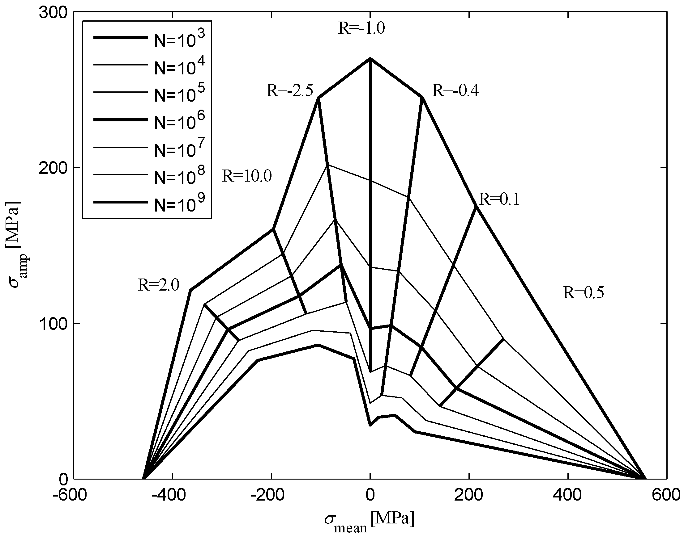
Constant amplitude and variable amplitude fatigue tests are available in the OptiDAT database [28] for geometry R04 MD (MultiDirectional laminate). This geometry has been selected because many fatigue tests are performed with this geometry. For composite materials the mean stress can have a significant influence on the fatigue properties. This is taken into account by estimation of SN-curves for different R-ratios and arranging these in a constant life diagram. The R-ratio is defined by:

$$R=\frac{{\sigma }_{\min }}{{\sigma }_{\max }}$$

(18)

where ${\sigma }_{\min }$ and ${\sigma }_{\max }$ are minimum and maximum stresses in a stress cycle respectively. A linear SN-curve model is used:

$$\log N_F=\log K-m\log \Delta \sigma +\epsilon$$

(19)

where N_F is the number of cycles to failure, $\Delta \sigma$ is the stress range and ε models the lack of fit and is assumed normal distributed with mean value zero and standard deviation ${\sigma }_{\epsilon }$. The constants K and m are material dependent parameters. If N constant amplitude tests and N₀ run-outs are available then m is obtained using the least squares method. The parameters log K and ${\sigma }_{\epsilon }$ can be estimated using the Maximum Likelihood Method, see Section 3. The statistical uncertainty represented by the standard deviations ${\sigma }_{\log K}$ and ${\sigma }_{{\sigma }_{\epsilon }}$ and the correlation coefficient ${\rho }_{\log K,{\sigma }_{\epsilon }}$ is obtained using (1).

Table 2 shows the estimated parameters in the SN-curves for different R-ratios with run-outs taken into account. The results show that log K and ${\sigma }_{\epsilon }$ can be assumed uncorrelated. It is noted that ${\sigma }_{\epsilon }$ represents the physical uncertainty and that ${\sigma }_{\log K}$ and ${\sigma }_{{\sigma }_{\epsilon }}$ represents the statistical uncertainty. Figure 1 shows the constant life diagram based on the estimated SN-curves.

Table 2. SN-curves for different R-ratios for geometry R04 MD.

R-ratio	Number of tests	Number of run-outs	m	$\mathbf{log}\mathit{K}$	${\mathit{\sigma }}_{\mathit{\epsilon }}$	${\mathit{\sigma }}_{\mathbf{log}\mathit{K}}$	${\mathit{\sigma }}_{{\mathit{\sigma }}_{\mathit{\epsilon }}}$
0.5	15	0	10.541	27.768	0.358	0.092	0.065
0.1	45	2	9.508	27.191	0.259	0.039	0.027
–0.4	28	0	7.582	23.398	0.435	0.082	0.058
–1.0	84	3	6.719	21.359	0.878	0.094	0.068
–2.5	10	2	11.983	35.231	0.633	0.197	0.143
10.0	34	0	22.211	58.664	0.644	0.110	0.078
2.0	6	3	29.686	73.780	0.354	0.143	0.103

Table 2. SN-curves for different R-ratios for geometry R04 MD.

R-ratio	Number of tests	Number of run-outs	m	$\mathbf{log}\mathit{K}$	${\mathit{\sigma }}_{\mathit{\epsilon }}$	${\mathit{\sigma }}_{\mathbf{log}\mathit{K}}$	${\mathit{\sigma }}_{{\mathit{\sigma }}_{\mathit{\epsilon }}}$
0.5	15	0	10.541	27.768	0.358	0.092	0.065
0.1	45	2	9.508	27.191	0.259	0.039	0.027
–0.4	28	0	7.582	23.398	0.435	0.082	0.058
–1.0	84	3	6.719	21.359	0.878	0.094	0.068
–2.5	10	2	11.983	35.231	0.633	0.197	0.143
10.0	34	0	22.211	58.664	0.644	0.110	0.078
2.0	6	3	29.686	73.780	0.354	0.143	0.103

Variable amplitude fatigue tests are also performed with geometry R04 MD. The load spectrum used is the Wisper and Wisperx spectra developed for representing the flap bending moment of a wind turbine blade. In order to calculate the accumulated damage D Miners rule for linear damage accumulation is used:

$$D={\displaystyle \sum _{i=1}^{N_C}\frac{1}{N_F\left(\Delta {\sigma }_i\right)}}$$

(20)

where N_C is the number of stress cycles with stress ranges $\Delta {\sigma }_i,i=1,2,...,N_C$. Fatigue failure occurs when the accumulated fatigue damage exceeds 1.

Figure 1. Constant life diagram for geometry R04 MD.

Figure 1. Constant life diagram for geometry R04 MD.

A limit state function including model uncertainty can be formulated by:

$$g=\Delta -{\displaystyle \sum _{i=1}^{N_C}\frac{1}{N_F\left(\Delta {\sigma }_i\right)}}$$

(21)

where Δ is a stochastic variable modeling the model uncertainty. Table 3 shows the variable fatigue tests performed and listed together with the estimated mean μ_Δ, standard deviation, σ_Δ and coefficient of variation, COV_Δ. The results show that except for the Wisper spectrum the estimated mean accumulated damage at failure is significantly below one and that the coefficients of variations are quite high. It is noted that the uncertainty for fatigue damage accumulation often is modeled by a Lognormal distribution in order to avoid negative values of Miners rule.

Table 3. Mean and standard deviations for estimated damage at failure for variable amplitude tests.

Spectrum	Number of tests	Mean ${\mathit{\mu }}_{\mathbf{\Delta }}$	Std. dev. ${\mathit{\sigma }}_{\mathbf{\Delta }}$	$\mathit{C}\mathit{O}{\mathit{V}}_{\mathbf{\Delta }}$
Wisper	10	0.90	0.54	0.60
Wisperx	13	0.28	0.20	0.72
Reverse Wisper	2	0.20
Reverse Wisperx	10	0.32	0.16	0.50
All	35	0.46	0.42	0.91

Table 3. Mean and standard deviations for estimated damage at failure for variable amplitude tests.

Spectrum	Number of tests	Mean ${\mathit{\mu }}_{\mathbf{\Delta }}$	Std. dev. ${\mathit{\sigma }}_{\mathbf{\Delta }}$	$\mathit{C}\mathit{O}{\mathit{V}}_{\mathbf{\Delta }}$
Wisper	10	0.90	0.54	0.60
Wisperx	13	0.28	0.20	0.72
Reverse Wisper	2	0.20
Reverse Wisperx	10	0.32	0.16	0.50
All	35	0.46	0.42	0.91

In summary this example illustrated how the following types of uncertainty can be modeled:

• Physical uncertainty is modeled by ε        (Normal distributed)
• Statistical uncertainty is modeled by $\log K$ and ${\sigma }_{\epsilon }$ (Normal distributed)
• Model uncertainty is modeled by Δ        (LogNormal distributed)

11. Conclusions

A probabilistic basis is described for reliability-based design of wind turbines. Probabilistic methods can be used as decision tool for design of structural wind turbine components, thereby ensuring a more uniform and economic design than obtained by traditional design using standards such as the IEC 61400 series. The following aspects are described:

• Identification and selection of structural elements to be included in the probabilistic basis: e.g., blades, tower, substructure and foundation;
• Identification and modeling by limit states of important failure modes;
• Stochastic models for the uncertain parameters;
• Recommendation of methods for estimation of the reliability;
• Recommendations for target reliability levels for the different groups of elements;
• Recommendation for considerations of system aspects and damage tolerant design.

An important aspect in obtaining wind turbine systems with high reliability and availability is to account for system reliability effects and to secure a system that is robust to unexpected incidents and errors. The application of a general framework for structural, risk-based robustness assessment to wind turbine systems is presented.

It is described how uncertainties in wind turbine design related to integrated design using computational models, statistical data from small (coupon) test specimens, results from a few full-scale tests and from prototype wind turbines can be accounted for using the Maximum Likelihood Method and a Bayesian approach. Further, this includes incorporation of site specific information on climatic parameters.

References and Notes

- Billinton, R.; Allan, R.N. The Reliability of Engineering Systems, 2nd ed.; Plenum: New York, NY, USA, 1992. [Google Scholar]
- Tavner, P.J.; Xiang, J.; Spinato, F. Reliability analysis for wind turbines. Wind Energy 2007, 10, 1–18. [Google Scholar] [CrossRef]
- Ronold, K.O.; Wedel-Heinen, J.; Christensen, C. Reliability-based fatigue design of wind-turbine rotor blades. Eng. Struct. 1999, 21, 1101–1114. [Google Scholar] [CrossRef]
- Madsen, H.O.; Krenk, S.; Lind, N.C. Methods of Structural Safety; Dover Publications: Mineola, NJ, USA, 1986. [Google Scholar]
- Joint Committee on Structural Safety (JCSS). Probabilistic Model Code. Available online: http://www.jcss.ethz.ch/ (accessed on 28 January 2010).
- Dueñas-Osorio, L.; Basu, B. Unavailability of wind turbines from wind induced accelerations. Eng. Struct. 2009, 30, 885–893. [Google Scholar] [CrossRef]
- Schittkowski, K. NLPQL: A FORTRAN subroutine solving non-linear programming problems. Annal. Operat. Res. 1986, 5, 485–500. [Google Scholar] [CrossRef]
- Lindley, D.V. Introduction to Probability and Statistics from a Baysian Viewpoint; Cambridge University Press: Cambridge, UK, 1976. [Google Scholar]
- Joint Committee on Structural Safety (JCSS). Risk Assessment in Engineering Principles, System Representation & Risk Criteria. Available online: http://www.jcss.ethz.ch/ (accessed on 28 January 2010).
- WAsP—the Wind Atlas Analysis and Application Program; Risø-DTU: Roskilde, Denmark. Available online: http://www.wasp.dk/ (accessed on 28 January 2010).
- Rackwitz, R. Optimization—the basis of code making and reliability verification. Struct. Saf. 2000, 22, 27–60. [Google Scholar] [CrossRef]
- Rackwitz, R. Risk control and optimization for structural facilities system. In Proceedings of 20th Conference on System Modelling and Optimization, Trier, Germany, July 2001; pp. 143–167.
- ISO 2394. General principles on reliability for structures. 1998. Available online: http://www.iso.org/iso/catalogue_detail?csnumber=7289 (accessed on 28 January 2010).
- Hayman, B. Approaches to damage assessment and damage tolerance for FRP sandwich structures. J. Sandw. Struct. Mater. 2007, 9, 571–596. [Google Scholar] [CrossRef]
- EN 1990. Basis of structural design. CEN 2002. Available online: http://www.techstreet.com/cgi-bin/detail?doc_no=BS_EN|1990_2002&product_id=1113608 (accessed on 28 January 2010).
- Baker, J.W.; Schubert, M.; Faber, M.H. On the assessment of robustness. Struct. Saf. 2008, 30, 253–267. [Google Scholar] [CrossRef]
- Madsen, H.O. Model updating in reliability theory. In Proceedings of ICASP5, Vancouver, Canada, May 1987; pp. 564–577.
- Schall, G.; Rackwitz, R. On the integration of multinormal densities over equalities. In Berichte zur Zuverlassigkeitstheorie der Bauwerke; Technical University Munich: Munich, Germany, 1988; Volume 83. [Google Scholar]
- Box, G.; Tiao, G.C. Bayesian Inference in Statistical Analysis; Wiley: New York, NY, USA, 1992. [Google Scholar]
- Raiffa, H.; Schlaifer, R. Applied Statistical Decision Theory; MIT Press: Cambridge, MA, USA, 1968. [Google Scholar]
- Sørensen, J.D.; Tarp-Johansen, N.J. Reliability-based optimization and optimal reliability level of offshore wind turbines. J. Offshore Polar Eng. 2005, 15, 1–6. [Google Scholar]
- Braam, H.; Rademakers, L.W.M.M. Guidelines on the Environmental Risk of Wind Turbines in the Netherlands; Report No. ECN-RX-04-013; ECN: Petten, Netherland, 2004. [Google Scholar]
- IEC 61400-1. Wind turbines—Part 1: Design requirements, 3rd ed. 2005. Available online: http://webstore.iec.ch/webstore/webstore.nsf/Artnum_PK/36653 (accessed on 28 January 2010).
- IEC 61400-3. Wind turbines—Part 3: Design requirements for offshore wind turbines. 2008. Available online: http://webstore.iec.ch/webstore/webstore.nsf/Artnum_PK/42608 (accessed on 28 January 2010).
- Tarp-Johansen, N.J.; Madsen, P.H.; Frandsen, S.T. Calibration of partial safety factors for extreme loads on wind turbines. In Proceedings of the European wind energy conference and exhibition (EWEC), Madrid, Spain, June 2003.
- Tarp-Johansen, N.J. Partial safety factors and characteristic values for combined extreme wind and wave load effects. J. Solar Energy Eng. 2005, 127, 242–252. [Google Scholar] [CrossRef]
- Toft, H.S.; Sørensen, J.D. Uncertainty on fatigue damage accumulation for composite materials. In Proceedings of the 22th Nordic Seminar on Computational Mechanics, Aalborg, Denmark, October 2009; pp. 253–256.
- OPTIMAT. Available online: http://www.wmc.eu/optimatblades.php (accessed on 28 January 2010).
© 2010 by the authors; licensee Molecular Diversity Preservation International, Basel, Switzerland. This article is an open-access article distributed under the terms and conditions of the Creative Commons Attribution license (http://creativecommons.org/licenses/by/3.0/).
Share and Cite
MDPI and ACS Style
Sørensen, J.D.; Toft, H.S. Probabilistic Design of Wind Turbines. Energies 2010, 3, 241-257. https://doi.org/10.3390/en3020241
AMA Style
Sørensen JD, Toft HS. Probabilistic Design of Wind Turbines. Energies. 2010; 3(2):241-257. https://doi.org/10.3390/en3020241
Chicago/Turabian StyleSørensen, John D., and Henrik S. Toft. 2010. "Probabilistic Design of Wind Turbines" Energies 3, no. 2: 241-257. https://doi.org/10.3390/en3020241