Mixed Over-Voltage Decomposition Using Atomic Decompositions Based on a Damped Sinusoids Atom Dictionary

Abstract

The main purpose of this paper is to establish a signal decomposition system aiming at mixed over-voltages in power systems. In an electric power system, over-voltage presents a great threat for the system safety. Analysis and identification of over-voltages is helpful to improve the stability and safety of power systems. Through statistical analysis of a collection of field over-voltage records, it was found that a kind of complicated signals created by mixing of multiple different over-voltages is difficult to identify correctly with current classification algorithms. In order to improve the classification and identification accuracy of over-voltages, a mixed over-voltage decomposition system based on the atomic decomposition and a damped sinusoid atom dictionary has been established. This decomposition system is optimized by using particle swarm optimization and the fast Fourier transform. Aiming at possible fault decomposition results during decomposition of the over-voltage signal, a double-atom decomposition algorithm is proposed in this paper. By taking three typical mixed over-voltages as examples, the validity of the algorithm is demonstrated.

1. Introduction

In an electric power system, an over-voltage could be generated by switch operation conditions, lightning and failure, etc. The main types of accidents in power systems are the insulation accidents caused by over-voltage incidents. Currently, with the continuous improvement of the power grid’s voltage grade, over-voltages can pose a greater hazard to the system equipment. Therefore, the feature extraction and identification algorithms for the over-voltages of the power system are of great significance in safeguarding the operations of the power grid. At the same time, the correct classification and identification of over-voltages can lay a solid foundation for the rapid intelligent inhibition of over-voltages.

Over-voltage online monitoring equipment has been widely used in power systems with different voltage grades and has recorded a large amount of field over-voltage waveforms. Generally speaking, the operation mode of over-voltage online monitoring equipments is as follows: considering the storage costs, the equipments stand by when the power system is working normally. In the event of switch operation or another disturbance, the monitoring equipment can record the waveform information of the signal at a certain sampling frequency and save it in the format of a group of discrete data. Therefore, generally, the waveform data recorded by the same monitoring equipment has a same time length.

Currently, a large number of scholars have carried out in depth research in the field of classification and identification of over-voltages and obtained a certain number of results [1,2,3]. However, in actual application, these algorithms cannot accomplish high-accuracy classification and identification. There are many shortcomings that must be overcome immediately. One of the important reasons for this is that these classification and identification algorithms have very high requirements for accuracy and integrity of the field waveforms recorded by the monitoring equipment. At the same time, these algorithms include one hidden precondition: one record must only include a single type of over-voltage.

For many years, Chongqing University has carried out a large number of studies in the online overvoltage monitoring and identification field. A series of effective monitoring equipments have been designed and installed in many power transformer substations. Through five years of data collection and accumulation, nearly 30,000 field over-voltage waveforms have been recorded. Though many of the over-voltage signal records can be identified, it is found out that a part of records are a kind of complicated signal mixed by multiple over-voltages, which are not easy to identify correctly.

Under certain conditions, if over-voltages occurred simultaneously, or within a shorter time interval and the time interval is less than the record time length, two or more kinds of over-voltage may be contained in one record. For this kind of complicated over-voltage record, the features cannot be extracted accurately by the current algorithms. Therefore, these kinds of over-voltage cannot be identified correctly, or just the most obvious type in these mixed signals may be identified.

In order to overcome the identification problem of the mixed over-voltages, it is very necessary to decompose the mixed signals according to their types before the classification and identification. In this paper, the concept of using an atomic decomposition based on a damped sinusoids atom dictionary to build a decomposition algorithm is introduced. Meanwhile, the Particle Swarm Optimization (PSO) and Fast Fourier Transform (FFT) are employed to reduce the computational complexity. Aiming at two possible incorrect results caused by the direct application of the atomic decomposition, an improved method of searching the best time support and a double- atom decomposition algorithm are proposed in this paper.

2. Mixed Over-Voltage

2.1. The Type of Mixed Over-Voltage

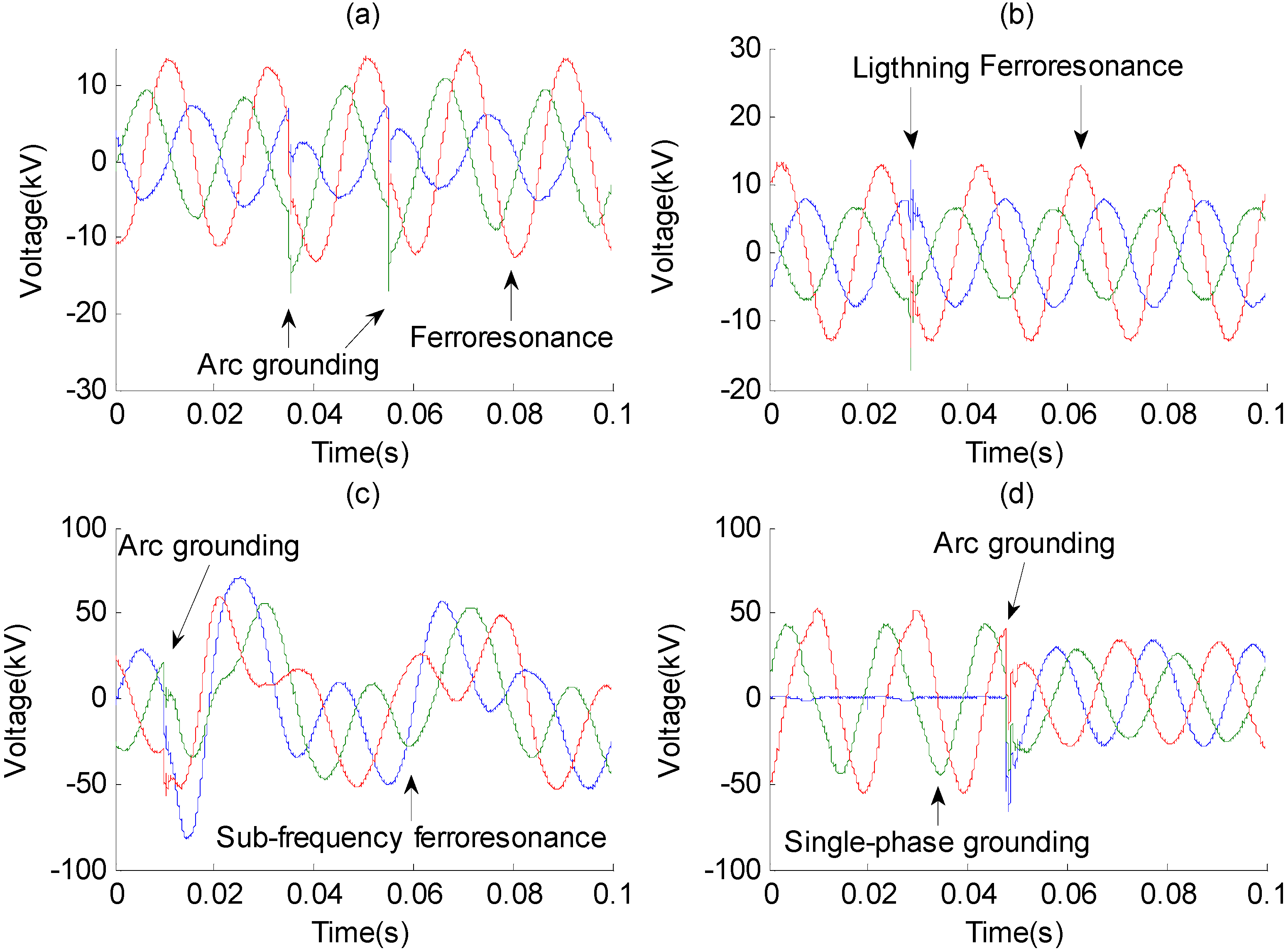
All the signals in this paper were recorded from a 110 kV/35 kV/10 kV transformer substation in Chongqing, China. Aiming at the identification of mixed over-voltages, these are divided into three types in this paper based on their waveform features.

The first one is a transient over-voltage mixed with a steady-state over-voltage. In this case, two over-voltages may occur simultaneously, such as a ferroresonance mixed with an arc grounding. Besides, two over-voltages may also appear one after another, for example, a ferroresonance caused by a switching operation.

The second one is a transient over-voltage mixed with a transient over-voltage. In this case, two transient waveforms are independent in the time domain. It is noted that two different transient over-voltages can rarely occur simultaneously, and this kind of mixed over-voltage has not been found in the existing measured database.

The third one is a steady-state over-voltage mixed with a steady-state over-voltage, for example, a ferroresonance caused by a disappearance of metal grounding. In this case, the two over-voltages are interconnected in the time domain. Four typical mixed over-voltages recorded in the power system are shown in the Figure 1.

Figure 1. Four typical mixed over-voltages: (a) Ferroresonance mixed with arc grounding; (b) Ferroresonance mixed with lightning; (c) Sub-frequency ferroresonance mixed with arc grounding; (d) Single-phase grounding mixed with arc grounding.

Figure 1. Four typical mixed over-voltages: (a) Ferroresonance mixed with arc grounding; (b) Ferroresonance mixed with lightning; (c) Sub-frequency ferroresonance mixed with arc grounding; (d) Single-phase grounding mixed with arc grounding.

Figure 1a shows the first type of mixed over-voltage imultaneously). For this signal, a ferroresonance occurs caused by the magnetizing inductance saturation of the electromagnetic potential transformer (PT) on the 10 kV bus. During the period of this fundamental ferroresonance, an arc grounding fault takes place on the 10 kV feeder. Therefore these two kinds of over-voltage are mixed together and recorded by the online monitoring device. It should be noted that this signal is also an example of the second type of mixed over-voltage, in which two independent arc grounding high-frequency transient oscillations occurs one after another. Figure 1b shows another example of this type of mixed over-voltage. In this figure, a fundamental ferroresonance takes place first on the 10 kV bus because of the saturation of 10 kV PT. Then a lightning strike takes places coincidentally on the feeder. At this moment, the voltage on the 10kV bus is recorded by the monitoring device. Thus this kind of mixed over-voltage is formed and stored in our field over-voltage database. Figure 1c shows another example of the first type of mixed over-voltage (two over-voltages appear one after another, not simultaneously). In this signal record, an arc grounding fault takes place at 0.01 s, which leads to that the 35 kV PT’s magnetizing inductances being saturated and therefore a sub-frequency ferroresonance take places. Figure 1d shows a single phase grounding over-voltage disappears with an arc grounding over-voltage, which is an example of the first type of mixed over-voltage.

2.2. Decomposition Target of Mixed Over-Voltage

For the transient and the steady-state over-voltages, the original waveforms need to be decomposed into the high frequency transient oscillation and the low frequency harmonic by their frequency and attenuation characteristics. During the process of the decomposition, the parameters of the starting time, frequency and damping factor need to be involved.

For the mixed over-voltage with multiple transient waveforms, the signal needs to be decomposed by its starting time. At the same time, the frequency and attenuation characteristic etc. parameters should also be involved in the decomposition process.

For the mixed over-voltage with multiple steady-state waveforms, the time domain, voltage amplitude value and frequency should be involved in the decomposition process.

The traditional general analysis methods used to process signals, such as the Fourier transformation [4,5] and the wavelet [6,7,8], cannot meet the requirements for the decomposition of mixed over-voltages. The Fourier transform can reflect the frequency domain characteristics of signals, but it cannot reflect the time domain characteristics of signals. It cannot locate the initiation time when the over-voltage occurs or disappears, which is important for the mixed over-voltage decomposition. The Fourier transform also cannot decompose a signal into a series of damped sinusoids. Therefore it is not suitable for the decomposition of high frequency sinusoidal oscillations, such as lightning and switching over-voltage. Short-time Fourier transformation can simultaneously reflect the time domain and frequency characteristics of the original signals, but the results may be greatly affected by the windowing function and the resolution is rather limited. The wavelet method is a constant multi-resolution analysis and cannot decompose the signals into a number of independent harmonics with a single frequency.

These algorithms try to express the original signals through a fixed basic function and they also lack consideration of the characteristics of the signals themselves. Therefore, in this paper, the over-voltage signal is decomposed based on the atomic decomposition algorithm and a well designed redundant damped sinusoid atom dictionary, so as to meet the requirement for the diversity of parameter types and the decomposition accuracy.

3. Atomic Decompositions

The Atomic Decomposition algorithm can decompose any signal into a series of linear expansions of atoms which are from a given redundant dictionary. Through this given redundant dictionary, a signal can be decomposed into any type of sub-signal. The principle of Atomic Decomposition can be described as the following contents. Define a set (D = {g_{γ (m)}; m = 1,2,…,K}), the element g_{γ (m)} is called atom, and D is called atom dictionary. Given a signal f, it can be decomposed by n atoms chosen from a redundant dictionary D:

$$f_n={\displaystyle \sum _{m=1}^n{c}_m{g}_{\gamma \left(m\right)}}$$

(1)

where the subscript γ (m) is the index of atoms, and c is the linear parameter used in signal reconstruction. The decomposition error is given by:

$${\sigma }_n\left(f,D\right)=\Vert f-f_n\Vert =\Vert f-{\displaystyle \sum _{m=1}^n{c}_m{g}_{\gamma \left(m\right)}}\Vert$$

(2)

It can be clear seen from the basic idea of the Atomic Decomposition algorithm, that the suitable construction of the atom dictionary and the way to find out the appropriate atoms are the key parts of the Atomic Decomposition algorithm.

3.1. Matching Pursuit

The way to identify the appropriate atoms is very important for the success of the Atomic Decomposition algorithm. The Matching Pursuit (MP) is one of the sparse approximation algorithms introduced by Mallat and Zhang in 1993 [9], Define D = {gγ}γ $\in$ Γ is an redundant atom dictionary, g_γ is the atom, which has the same length with the signal, and ||g_γ|| = 1. The MP algorithm can find the best approximation atom g_γ0 from the atom dictionary by calculating the inner product between the atom and the signal f:

$$\left|\langle f,g_{\gamma 0}\rangle \right|=\sup \left|\langle f,g_{\gamma }\rangle \right|$$

(3)

Thus the signal f can be described as:

$$f=\langle f,g_{\gamma 0}\rangle g_{\gamma 0}+R^{1}f$$

(4)

where <f, g_γ0> g_γ0 is the signal’s projection on the atom g_γ0, R¹f is the residue. Then, set the residue be the new signal f, repeat the decomposition algorithm in the same way. In each iteration, an atom and a new residue will be found. The MP will stop when the energy of the residue is less than a given threshold.

In the actual calculation, a correlation coefficient λ is defined to describe the approximation between the atom and signal. The best approximation atom is the one of the largest λ in the dictionary:

$$\lambda =\frac{\left|\langle f,g_{\gamma }\rangle \right|}{\Vert f\Vert \Vert g_{\gamma }\Vert }$$

(5)

Matching Pursuit has been successfully used in various fields, such as audio processing [10,11], image and video coding [12,13,14], and the detection of oscillatory transients [15].

3.2. Dictionary of Damped Sinusoids

The common types of atomic dictionary for Matching Pursuits include the Gabor dictionary [9] and the damped sinusoidal dictionary [16]. Over-voltage signals are composed of sinusoidal oscillations and harmonics, which can be represented as the sinusoidal with an increasing or decreasing amplitude or just the pure sinusoidal. In order to analyze and decompose this complex signal, the atoms in the dictionary employed in this paper are the parameterized damped sinusoidal atoms, and furthermore, two step functions are added to the original damped sinusoids expression, to make this dictionary have the ability to reflect the time domain features of the over-voltage signals. The expression is shown as:

$$g_{\gamma }(t)=A_{\gamma }\cos \left(2\pi f_{\gamma }t+{\varphi }_{\gamma }\right)e^{-\rho \left(t-t_{sp}\right)}\times \left[u\left(t-t_{sp}\right)-u\left(t-t_{ep}\right)\right]$$

(6)

where γ = {f, φ, ρ, t_sp, t_ep} is the set of parameters, f is the frequency, φ is the phase angle, ρ is the damping factor, t_sp is the starting time, t_ep is the ending time. The range of each parameter is listed in the Table 1. It should be noted that the over-voltage signal is a series of discrete data, recorded through online over-voltage monitoring equipment and the sample frequency is 200 kHz. Therefore the length of time between neighbor samples is 0.000005 s, the total sample points of all the example in this paper is 20,000.

Table 1. Range of parameters.

Parameters	Range
F	0 Hz~100 kHz
Φ	π/180~2 π
Ρ	−5000~5000
tsp	0 s~0.099995 s
tep	tsp + 0.000005 s~0.1 s

Table 1. Range of parameters.

Parameters	Range
F	0 Hz~100 kHz
Φ	π/180~2 π
Ρ	−5000~5000
tsp	0 s~0.099995 s
tep	tsp + 0.000005 s~0.1 s

It can be calculated that the scale of the atom dictionary is:

$$100001\times 360\times 10001\times {\displaystyle \sum _{n=1}^{19999}n}\approx 7.2\times {10}^{19}$$

(7)

It is clear that the number of atoms in the damped sinusoid atom dictionary is up to 7.2 × 10¹⁹, and each step of the decomposition needs to traverse the whole atom dictionary, which causes the MP algorithm to lose its practical value. It is very necessary to optimize this algorithm to reduce the computational complexity.

4. Optimization and Improvement of Matching Pursuit

From the above analysis, it can be found that the MP algorithm cannot be directly applied to the selection of the atoms. Meanwhile, the results obtained from the direct application of MP decomposition are not necessarily the correct or expected results. In this paper, the MP algorithm is optimized to improve the decomposition accuracy and avoid the decomposition errors.

4.1. Matching Pursuit Optimized by Particle Swarm Optimization

The particle swarm optimization (PSO) was proposed by Eberhart and Kennedy in 1995, and is a new evolutionary computation technique developed in recent years. Like other evolutionary computation techniques, the PSO calculation starts from a group of random solutions, and the optima are searched by updating these solutions in iteration. In addition, this algorithm is an optimized algorithm with memory capacity. PSO has received widespread attention in academic circles because of its advantages such as easy realization, high accuracy and rapid convergence, etc., and it has shown its superiority in the resolution of actual problems.

The PSO can be described as follows: in a swarm consisting of N particles in a K dimensional space, each particle is one solution to optimize a problem. The particle coordinate can be defined as X. In addition, each particle has a velocity parameter to determine its movement direction and distance. Each particle has a fitness value calculated by the fitness function which is to be optimized.

In the iterative calculations of PSO, the best coordinate for each particle which has achieved so far, is stored in the personal best value pBest. The best coordinate for the whole swarm which has ever achieved is stored in a global best value gBest. The particle can continuously update its position and movement velocity according to these two parameters.

In this paper, the atomic parameters are quantified as the coordinates of the particles, and the correlation coefficient λ between the atom and signal is used as a fitness value. The flying velocity can be obtained by the random initial assignment. In this way, the calculation speed of MP algorithm can be optimized by PSO. The updating algorithm of the particle’s coordinate is as follows:

$$\begin{array}{cc}V\left(i,j\right)=& w\times V\left(i,j\right)+C1\times rand\times \left(pBest(i,j)-X\left(i,j\right)\right)\\ & +C2\times rand\times \left(gBest(i)-X\left(i,j\right)\right)\end{array}$$

(8)

$$X\left(i,j\right)=X\left(i,j\right)+V\left(i,j\right)$$

(9)

where, V(i, j) {i = 1,2,…N, j = 1,2,…,K} is the speed of the jth particle on the ith dimension, X(i, j) {i = 1,2,…N, j = 1,2,…,K}is the coordinate of the jth particle on the ith dimension, C1 and C2 are the learning speed, in this paper C1 = C2 = 2, gBest(i) is the coordinate of the global best particle on the ith dimension, w is the weight, in this paper w is 0.7298, and rand is the random number between 1 and 2. The specific calculation steps of PSO-MP algorithm are shown as follows:

1)

Decode the parameters f, φ, ρ, t_sp, t_ep to form the initial particles. Each particle is created randomly, which covers the entire range of these parameters;

2)

Calculate the fitness value of each particle based on Equation (5). Record the position of each particle as its pbest, then find the fittest particle (find the largest λ) and mark it as the gbest;

3)

Initialize the speed of all the particles. Then update the position of each particle by Equation (8) and (9). Update the global fitness value gbest and the personal best position pbest;

4)

Repeat this cycle. The best particle is obtained after the particles fly for 40 times.

The numbers of particles and iterations of PSO can affect the optimization results directly. According to the experience of PSO algorithm application, the number of particles is usually set between 10 and 40. The higher the number of particles, the longer the computation time is. A large number of mixed over-voltages are adopted as examples to compare the decomposition results when the numbers of particles are 30, 40 and 50. The better number of the particles is chosen as 40 in this paper according to the statistical analysis. In the same way, the number of iterations for each atom in PSO-MP algorithm is decided by statistical analysis using a large number of testing examples.

4.2. Matching Pursuit Optimized by Fast Fourier Transform

Because the atomic decomposition algorithm used in this paper is based on the damped sinusoid dictionary, the expression of this atomic dictionary involves five parameters, i.e., γ = {f, φ, ρ, t_sp, t_ep}, which shows that the frequency parameter f is just the frequency value of the sinusoid atom. In order to reduce the computational complexity of the MP algorithm, a frequency pre-calculation approach is presented in this paper. Based on the frequency characteristic, the Fast Fourier transform can be used for the calculation of atomic parameters, which can be applied to reduce the calculation complexity of MP algorithm. The calculation process of this method is as follows:

1)

Calculate the frequency spectrum A(f) of the current signal to be decomposed using FFT;

2)

Find the frequency parameter with the maximum amplitude in the frequency spectrum;

3)

Quantify the frequency spectrum as the atomic frequency parameters, which means the MP algorithm can find the best atom from the new atom group, in which all the atom’s frequency are f_m.

Based on this method, f in the original atom group can be ignored. The new established atom only includes four parameters i.e., γ = {φ, ρ, t_sp, t_ep}. This method validly decreases the traversal atomic dictionary scale for the MP algorithm. The final calculated results are still obtained through an MP algorithm search. FFT calculation is only used to guide the search direction of the parameter space during the calculation of MP algorithm and would not affect the final calculated results. A large amount of actual data calculations show that pre-calculation of atomic frequency by FFT can both validly reduce the computational complexity of MP algorithm indeed and ensure the correctness of the calculated results.

4.3. Improved Optimal Time Support Search Algorithm

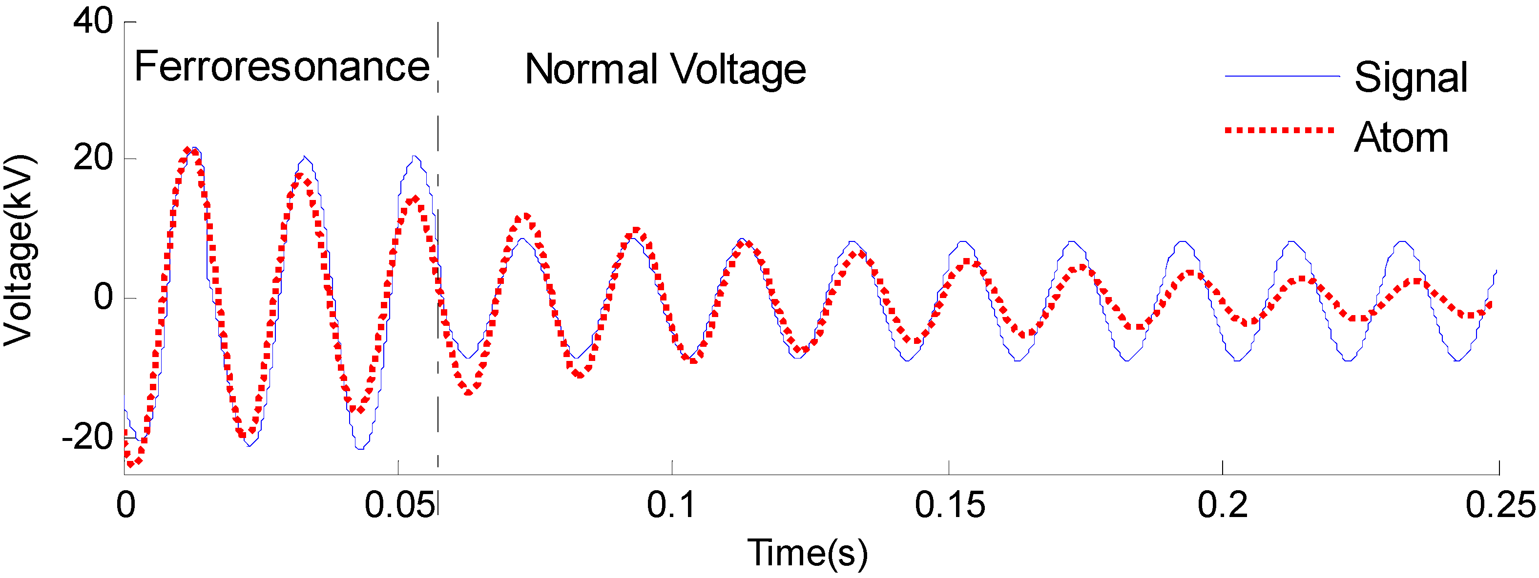
In the actual decomposition, some incorrect decompositions could occur. For example, the signal shown in Figure 2 is a mixed over-voltage. In this signal, a ferroresonance exists until 0.05 s, after that the ferroresonance disappears and the voltage recovers to the normal situation. As for this signal, the correct decomposition result should be a pure sinusoidal wave which has a larger amplitude within 0~0.05 s and the pure sinusoidal wave which has a normal amplitude value within 0.05~0.25. However, when using MP to decompose the signal, the best approximant atom depends on the inner product between the atom and signal overall time domain. The bigger the inner product, the better the atom is. Based on this judgment, a damped sinusoid covering the overall time domain is obtained, but the original signal’s true internal physical phenomena are not reflected, which is shown in Figure 2. Aiming at this incorrect decomposition, some solutions have been proposed.

Figure 2. An incorrect decomposition result of time support.

Figure 2. An incorrect decomposition result of time support.

Lovisolo proposed an algorithm by reducing the time support of the atom by box-windowing the signal in order to verify whether a new time support can produce a better fit between the atom and the current residue [17,18,19]. This algorithm focused on the local approximation of the signal instead of the global approximation. Although the incorrect decomposition was solved successfully in this improved algorithm method, there are still many faults in its practical application. In such an algorithm, when searching for the best local time support, the search must begin from the signal’s starting point or ending point sample by sample. In this paper, all over-voltage records include 20,000 sampling points, which means that the MP has to search through thousands of samples before the correct time support is found.

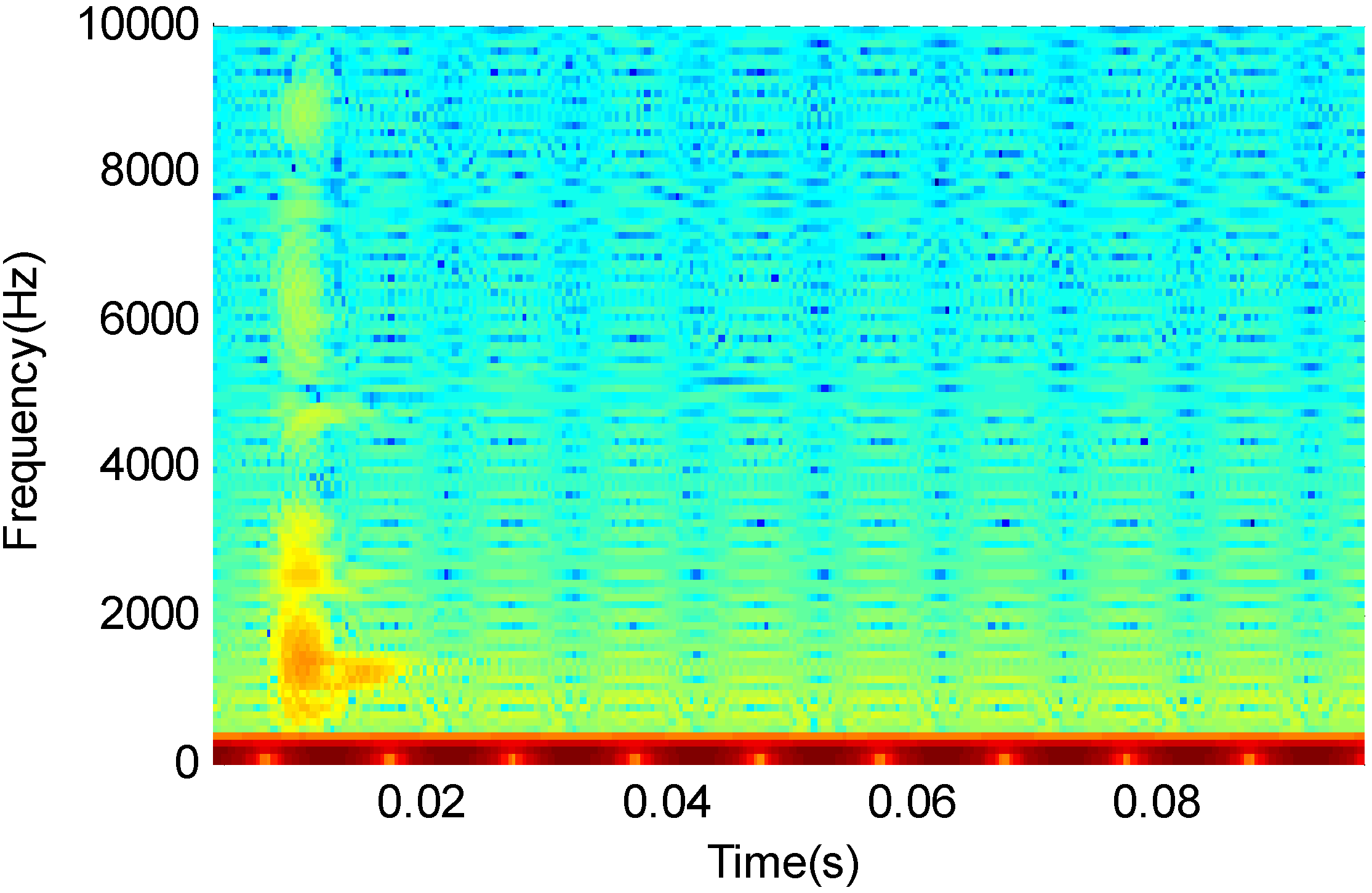
In order to reduce the computational complexity of the optimal time support research algorithm, some other fast algorithms are applied to pre-estimate the starting time and ending time of the best time support, so as to reduce the requested search scope. Generally, the starting or ending point of the best time support is the time that the over-voltage appears or disappears. Thus the characteristic on the signal waveform is that there is a high frequency transient oscillation occurs or a phase-step phenomenon is shown on the fundamental frequency harmonic. The starting point of the best time support can be located as follows:

1)

Obtain the time-frequency spectrum STFT(t, f) through Short Time Fourier Transformation. An example is shown in Figure 3. It is a time-frequency spectrum of switching no-load line. Calculate the amplitude-time spectrum AvsT(t) of high frequency (>400 Hz):

$$AvsT\left(t\right)={\displaystyle \underset{400}{\int }STFT(t,f)}df$$

(10)

2)

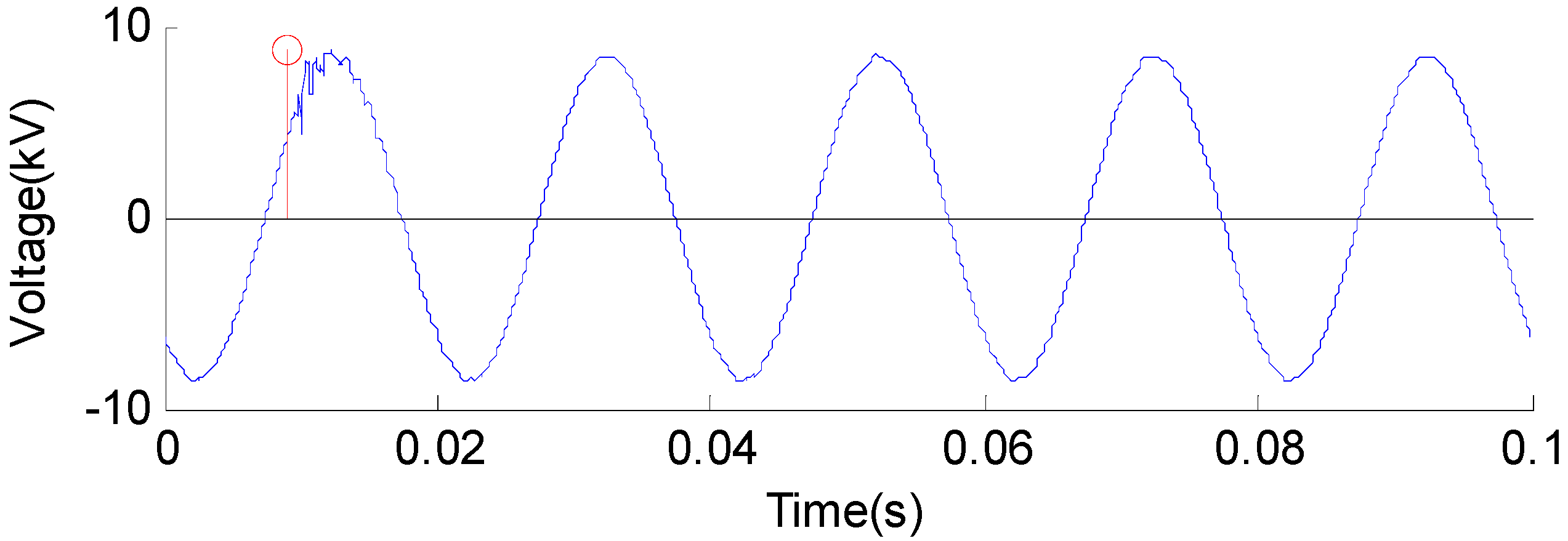
Find the local extreme point in the amplitude-time spectrum AvsT(t). Each local extreme marks the emergence of high-frequency oscillations. For example, the starting time of the switching no-load line over-voltage is shown as the red marker in Figure 4.

Figure 3. Time-frequency spectrum of switching no-load line.

Figure 3. Time-frequency spectrum of switching no-load line.

Figure 4. Location of extreme point in switching no-load line over-voltage.

Figure 4. Location of extreme point in switching no-load line over-voltage.

The step points of the fundamental frequency harmonic are obtained in this paper through a digital filter and Hilbert Transform. These step points are the time points that the over-voltage appears or disappears. The final disturbance points are composed of these two kinds of time points, and the possible duplicate points must be combined. The best time support is searched around these time points instead of the starting and ending point.

4.4. Double-Atom Decomposition Algorithm

Because a variety of over-voltage signals are mixed with complicated waveforms, and the best atom is searched only by its inner product with signal, the decomposition results may not reflect the correct physical phenomena of the signals sometimes.

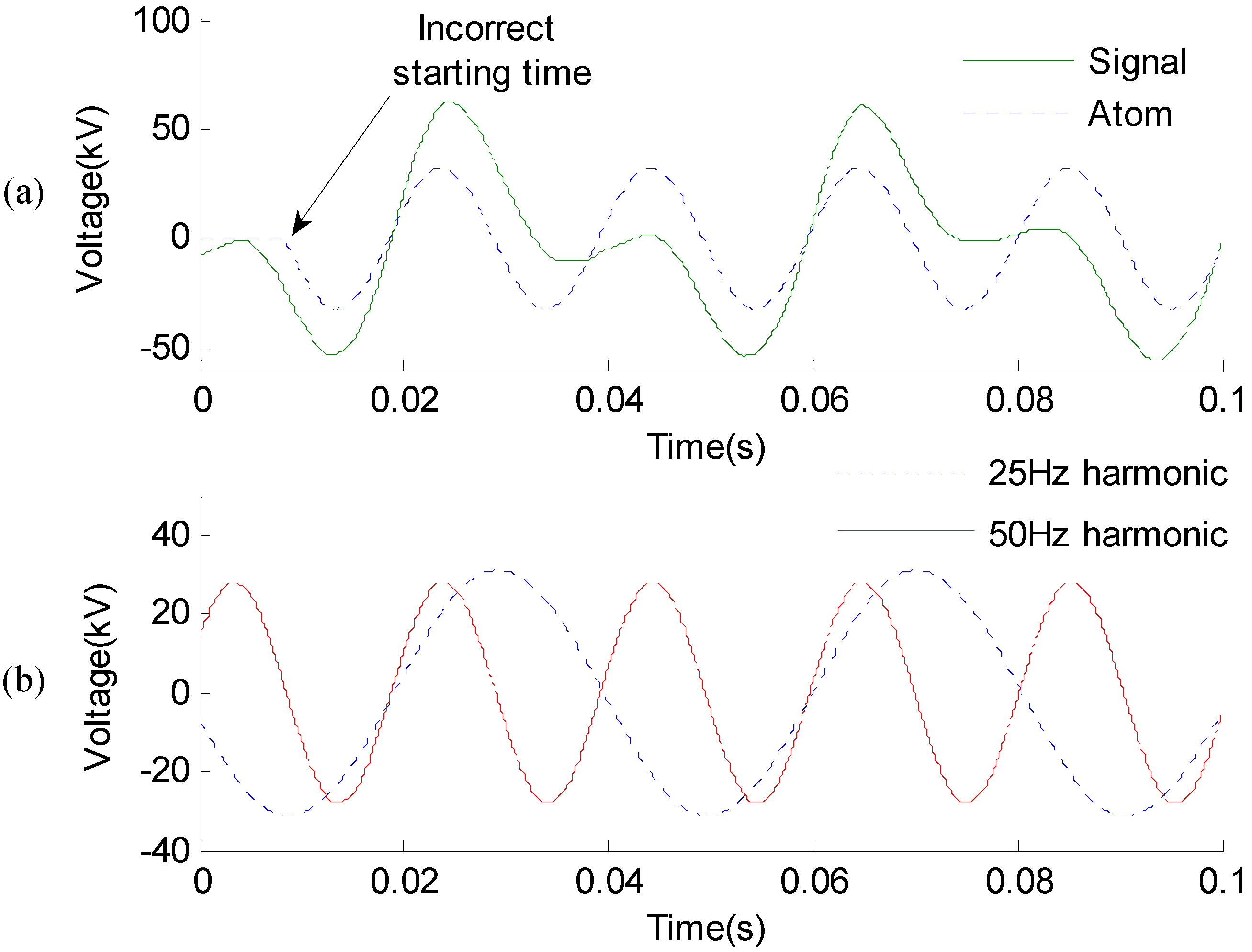
An incorrect decomposition is shown in Figure 5a. The target signal to be decomposed in the figure is a sub-frequency ferroresonance over-voltage. The result obtained by the MP algorithm is a sinusoid atom with incorrect starting time, while the correct decomposed result should be a pure sinusoid waveform with its starting time at 0 s. The main reason causing this incorrect decomposition is that the two main harmonic components (50 Hz and 25 Hz) of the sub-frequency ferroresonance have similar amplitude at the beginning, and the difference of the phase is close to 1 π, as shown in Figure 5b. The amplitudes of these two components (50 Hz and 25 Hz) are offset each other at the beginning, which may mislead the MP algorithm in searching the correct starting time t_sp.

Figure 5. (a) An incorrect decomposition of sub-frequency ferroresonance; (b) Two main harmonic components of sub-frequency ferroresonance.

Figure 5. (a) An incorrect decomposition of sub-frequency ferroresonance; (b) Two main harmonic components of sub-frequency ferroresonance.

The best time support cannot be searched based on the 50 Hz atom only (or 25 Hz atom either). Therefore, in this paper, a new method in which the two original atoms (50 Hz atom and 25 Hz atom) are combined together to form a new one is proposed, which is more similar to the signal that needs to be decomposed. Thus, the best time support is searched based on this new atom. This new atom can be expressed as follows:

$$\begin{array}{cc}{g}_{\gamma }^{\prime }(t)=g_{\gamma }(t)+g_r^{\prime }(t)=& A_{\gamma }\left[\cos \left(2\pi f_{\gamma }t+{\phi }_{\gamma }\right)e^{-\rho \left(t-t_{sp}\right)_{\gamma }}+\cos \left(2\pi f_{\gamma +1}t+{\phi }_{\gamma +1}\right)e^{-{\rho }_{\gamma +1}\left(t-t_{sp}\right)}\right]\\ & \times \left[u\left(t-t_{sp}\right)-u\left(t-t_{ep}\right)\right]\end{array}$$

(11)

where the new atom g_γ’ is formed by two original atoms g_γ and g_γ+1. The parameter set of the new atom g_γ, is γ = {f_γ, f_γ+1, φ_γ, φ_γ+1, ρ_γ, ρ_γ+1, t_sp, t_ep}. Thus, the atom g_γ, consists a new dictionary, in which each atom is composed by two atoms. Therefore, searching the best atom from this new dictionary is called as double-atom decomposition method in this paper.

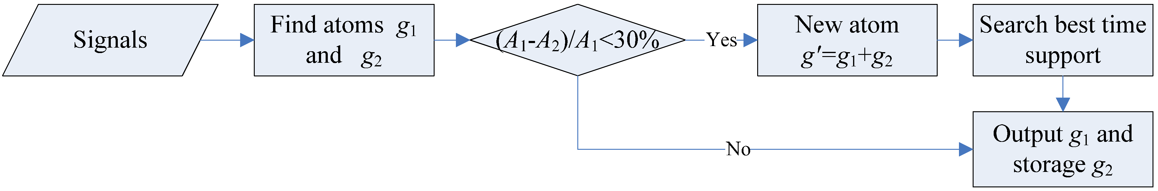
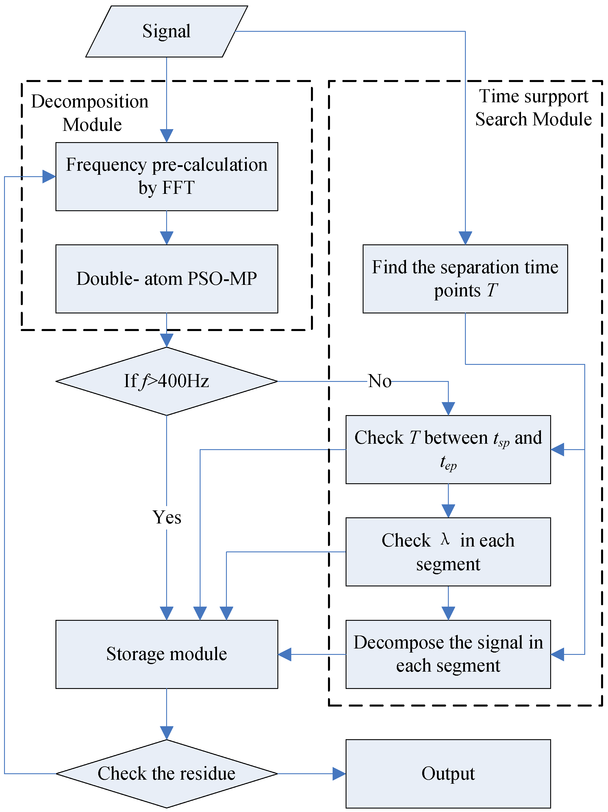
The double-atom decomposition method may unavoidably cause a rapid increase of the computational complexity. The calculation time is so long that the algorithm may lose its actual application value even if the algorithm is optimized by PSO and FFT. In order to reduce the computational complexity, the algorithm of double-atom is modified as follows and shown in Figure 6:

Figure 6. Block diagram of the double-atom decomposition algorithm.

Figure 6. Block diagram of the double-atom decomposition algorithm.

1)

Decompose the signal through PSO-MP into atom g₁ and the residual R₁, and then decompose the residual R₁ into atom g₂ and a new residual R₂;

2)

If the amplitudes of these two atoms are close enough (the difference of two amplitude is less than 30%), combine them together to form a new atom g’ (the time domain of the new atom is the overlapping part of the two atoms on the time domain). Otherwise, output atom g₁ is the result, and store atom g₂ to the background. Through the statistics of the field signals which need to be decomposed by the double-atom decomposition, it is found that the amplitude difference between two main harmonics is almost less than 15%. In order to make sure the precision and accuracy rate of the decomposition. The threshold used in this algorithm is set as 30%;

3)

Expand the new atom’s time domain by decreasing the starting time t_sp and increasing the ending time t_ep, and check that whether a new time support produces better fit between the atom g’ and the original signal. If the new time domain cannot cover the whole time domain of the original signal, individually add the time domain of the first atom in the two atoms and then check the approximation effect;

4)

Output the result and store the second atom in the background;

5)

In the next cycle, the atom g₂ stored in the background will be used directly, and the decomposition calculation in the first step will be omitted.

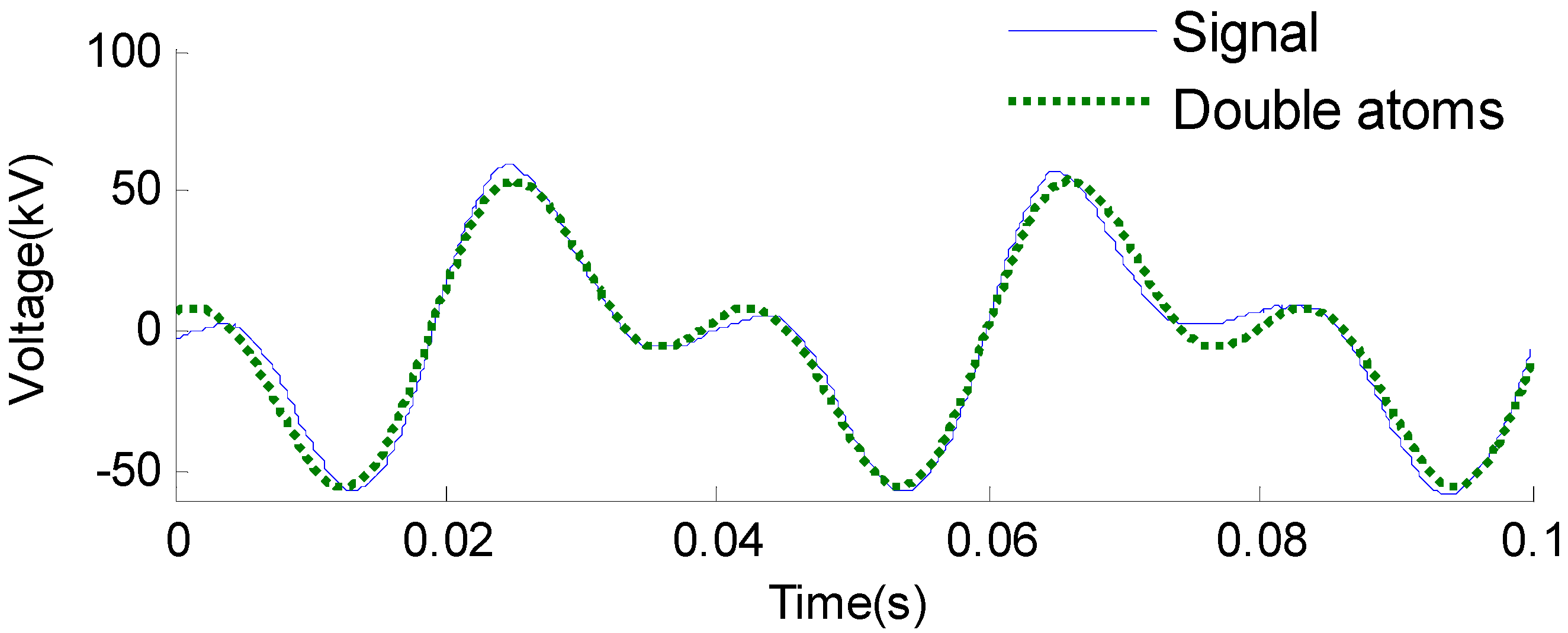
A sub-frequency ferroresonance over-voltage is decomposed by double-atom decomposition algorithm as an example in Figure 7. It is clear that the starting time t_sp of the new atom is 0 s, which is the expected correct decomposition.

Figure 7. Double-atom decomposition result of sub-frequency ferroresonance.

Figure 7. Double-atom decomposition result of sub-frequency ferroresonance.

5. Decomposition Algorithm for Mixed Over-Voltage

The decomposition system for mixed over-voltages built in this paper includes two branches. The high frequency oscillatory transients are decomposed by the double-atom PSO-MP directly, while for the low-frequency harmonic, it is not only decomposed by the double-atom PSO-MP, but it also must be checked for decomposition errors like the example shown in Figure 2. The main reasons of using such an algorithm are as follows:

1)

In most cases, the high-frequency oscillation component will attenuate rapidly and become zero or a very small amplitude value before the next over-voltage occurs. The step phenomenon hardly occurs on a high-frequency oscillation;

2)

It is known from the decomposition target that the decomposition algorithm of mixed over-voltages is built for the over-voltage identification in this paper. The low frequency harmonic components have greater impact on the recognition rate. Therefore, low frequency components need to be decomposed more precisely.

In order to make sure the decomposition algorithm has high precision and is practical, and reduce the computational complexity as much as possible, the mixed over-voltage decomposition system built in this paper is shown in the following Figure 8.

Figure 8. Block diagram of the decomposition algorithm.

Figure 8. Block diagram of the decomposition algorithm.

1)

In the decomposition module shown in Figure 8, the over-voltage signal is decomposed in the decomposition module. In this module, three optimization measures are involved: frequency pre-calculation (see Section 4.2), Particle Swarm Optimization (see Section 4.1), double-atom decomposition algorithm (see Section 4.4).

2)

Check the frequency of the current atom, as shown in Figure 8. If the frequency f > 400 Hz, the atom is a high frequency oscillatory transient in this iteration. The result is output to the storage module. Otherwise, the atom is a low frequency harmonic. The result is output to the best support search module.

3)

The best support search module shown in Figure 8 includes four steps:

• Find out how many over-voltages occur in the original waveform (see Section 4.3). Assume M is the number of the over-voltages and T (T = T₁,T₂,T₃,…,T_M) are the time points when they occur. In order to facilitate the description below, T represents the separated time points in this paper.
• Check out if there are any separation time points in the time domain of the current atom (between tsp and tep). Assume Ts (Ts$\subseteq$T; T_s = T_s1,T_s2,T_s3,…,T_sm) are the separated time points existing between t_sp and t_ep, m is the number of these separated time points (m ≤ M, t_sp ≤ T_s1, T_sm ≤ t_ep). If there is no such separated time points T_s exists (m = 0), the current atom is output to the storage module.
• If m > 0, divide the signal and atom into m + 1 segment by the separated time points T_s, t_sp and t_ep. Calculate the correlation coefficient λ in each segment by Equation (5). The number of correlation coefficients is also m + 1. If the values of these λ are close from each other, output the result to the storage module. Otherwise the signal is re-decomposed.
• Decompose the signal thought double-atom PSO-MP in each segment, then search the best time support of these atoms (see Section 4.3). Output the result to the storage module.

4)

All the atoms are stored and organized by their frequency. If the frequency is higher than 400 Hz, the atoms are combined by their starting time t_sp to compose an oscillatory transient. If the frequency is lower than 400 Hz, each atom represents a low frequency harmonic. Thus these low frequency atoms are stored as the results directly.

5)

Compare the energy of the residual with a given threshold to decide when the cycle is stopped.

6. Applications of the Decomposition Algorithm

Four typical mixed over-voltages are decomposed as the examples to verify the effectiveness of this mixed over-voltage decomposition algorithm. The four waveforms shown in Figure 9a are the sub-frequency ferroresonance, two decomposition results and residual from top to bottom. The two decomposition results respectively present the 50 Hz harmonic and 25 Hz harmonic of the original signal. The time of starting point of these two waves is 0 s. Such result is obtained though double-atom PSO-MP algorithm.

Figure 9. (a) Decomposition of sub-frequency ferroresonance; (b) Decomposition of single phase grounding mixed with arc grounding over-voltage.

Figure 9. (a) Decomposition of sub-frequency ferroresonance; (b) Decomposition of single phase grounding mixed with arc grounding over-voltage.

The four waveforms shown in Figure 9b are the original waveform of the over-voltage, two decomposition results, and residual from top to bottom. The over-voltage signal is the phase A signal of the mixed over-voltage shown in Figure 1d. The first result is a fundamental frequency (50 Hz) harmonics with the norm amplitude (35 kV), and its starting time t_sp is 0.047 s. The second result is an oscillatory transient represent the arc grounding over-voltage at 0.047 s.

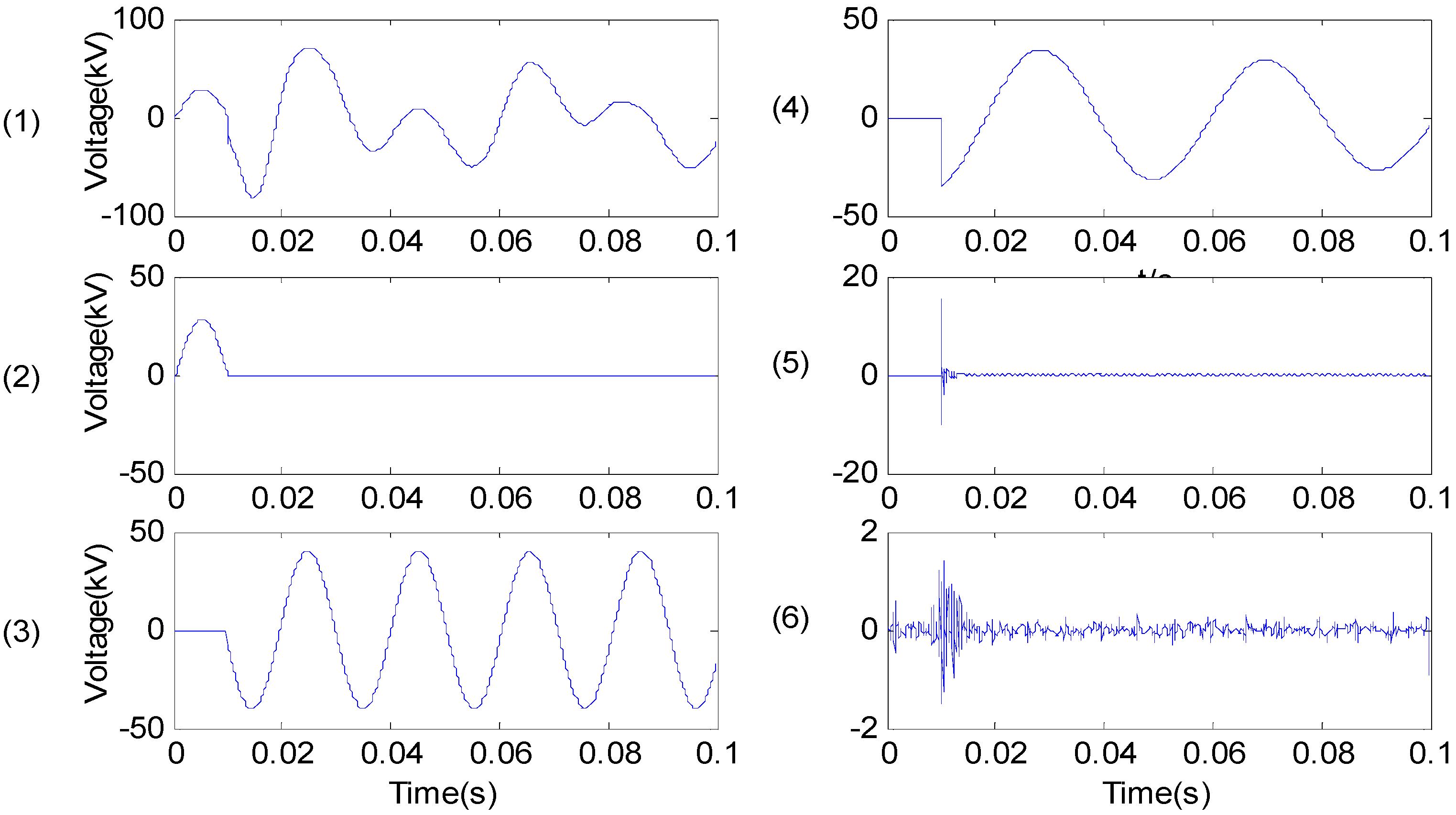
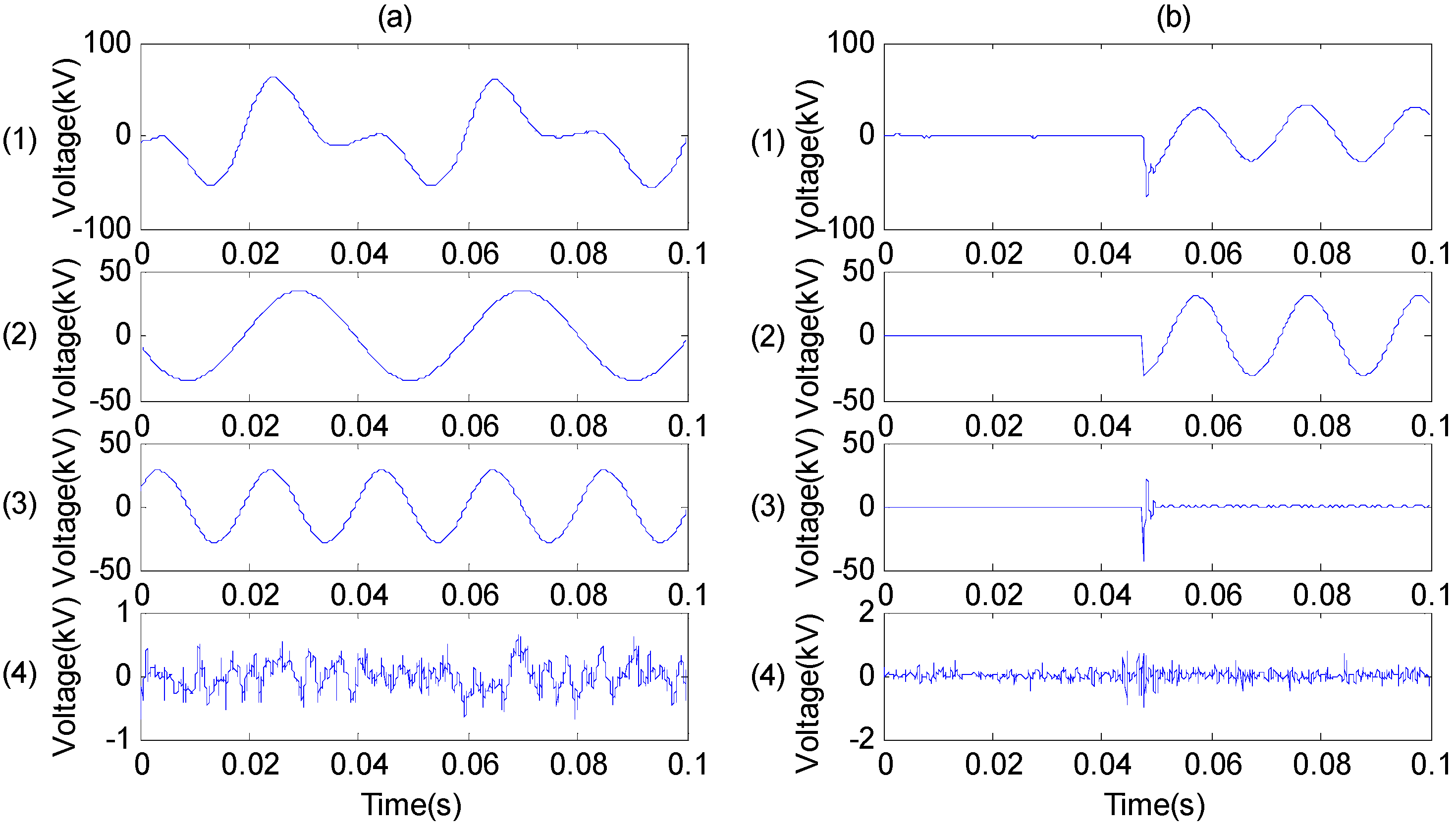
Figure 10 shows the original waveform of over-voltage, four decomposition results, and the residual from index (1) to (6). The original signal is a sub-frequency ferroresonance caused by an arc grounding which occurs at 0.01 s. The first decomposition result is the normal signal of 0~0.01 s; the second and third decomposition results are 50 Hz and 25 Hz harmonic of the sub-frequency ferroresonance after 0.01 s, and the fourth decomposition result is the arc grounding transient oscillation waveform at 0.01 s.

Figure 10. Decomposition of sub-frequency ferroresonance mixed with arc grounding over-voltage.

Figure 10. Decomposition of sub-frequency ferroresonance mixed with arc grounding over-voltage.

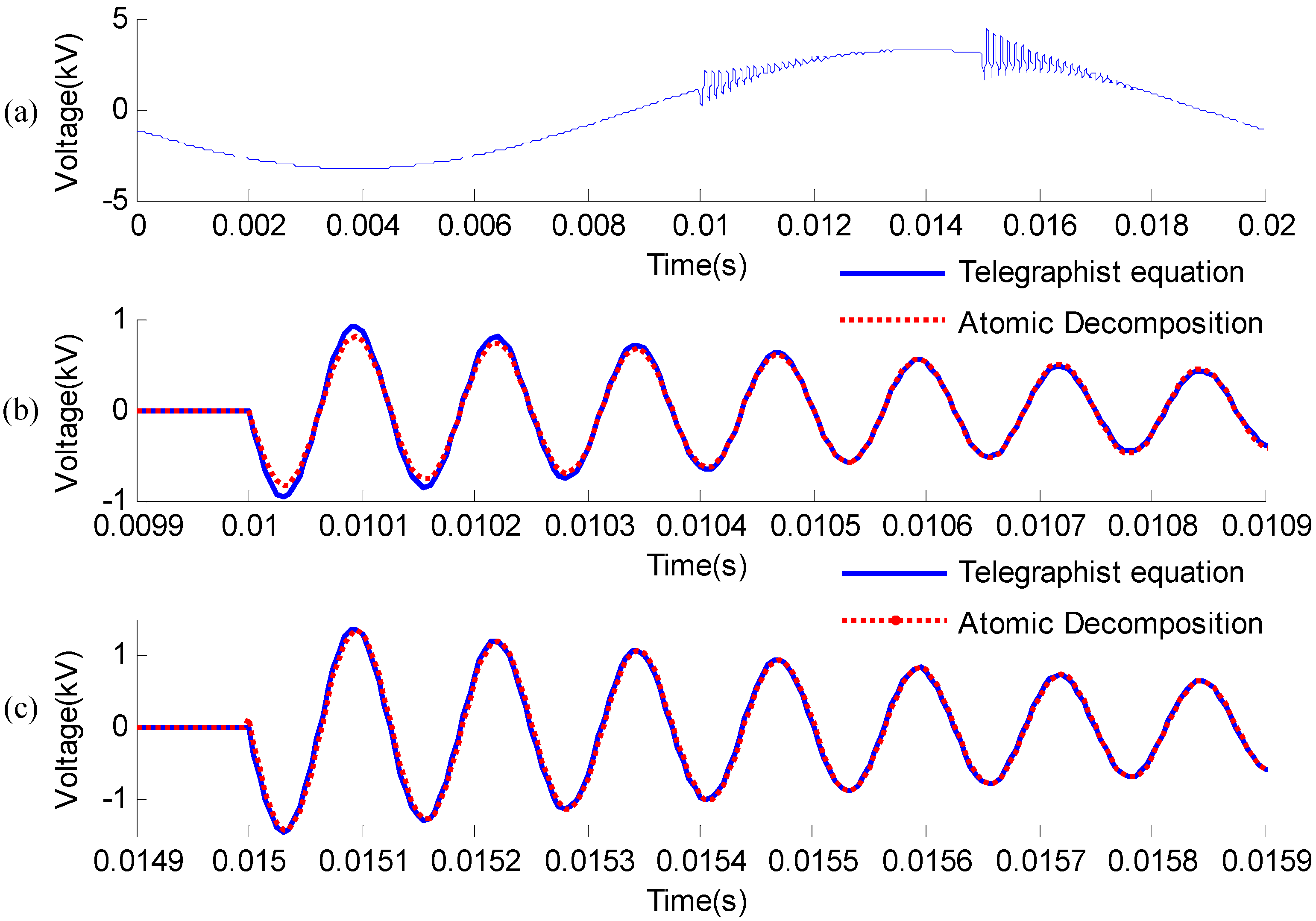
Furthermore, in order to verify the proposed method, a comparison between the proposed decomposition method and the Telegraphist equation is given. The simulation model is shown in Figure 11.

Figure 11. The simulation model.

Figure 11. The simulation model.

$$V(t)=10\cos (100\pi t+\pi )+5\cos \left(16000\pi t+\frac{\pi }{2}\right)e^{-1000\left(t-0.01\right)}\times u\left(t-0.01\right)$$

(12)

The voltage source is the combination of a power frequency voltage source and a high frequency oscillation voltage source, and the expression of the voltage is shown in Equation (12). The voltage wave will travel through a resistor and a wave impendence with a length of 500 km. The end of the wave impendence is connected with a zero load. The V(t) of the point between the resistor and the wave impendence can be obtained, which is shown in Figure 12a. Because there is a reflection at the end of the wave impendence, Figure 12a show s an original signal that contains a high frequency oscillation (at 0.01 s) and its reflection (at 0.015 s). Figure 12b,c are these two high frequency oscillations obtained from Telegraphist equation and Atomic Decomposition. It is clear that the decomposition results obtained from Atomic Decomposition are highly similar to the results obtained from the Telegraphist equation. It is thus verified that the decomposition algorithm has a high value in practice.

Figure 12. The contrast between the Telegraphist equation and Atomic Decomposition. (a) The waveform of a high frequency oscillation and its reflection; (b) The contrast between Telegraphist equation and Atomic Decomposition of original high frequency oscillation; (c) The contrast between Telegraphist equation and Atomic Decomposition of the reflection of high frequency oscillation.

Figure 12. The contrast between the Telegraphist equation and Atomic Decomposition. (a) The waveform of a high frequency oscillation and its reflection; (b) The contrast between Telegraphist equation and Atomic Decomposition of original high frequency oscillation; (c) The contrast between Telegraphist equation and Atomic Decomposition of the reflection of high frequency oscillation.

7. Conclusions

This paper is based on the use of the MP algorithm to set up a decomposition system for mixed over-voltage signals. The mixed over-voltage is an amplitude signal including a variety of different types in one waveform record. For this mixed over-voltage signal, currently, the existing algorithms cannot be used for correct classification and identification. In order to solve this problem, it is necessary to decompose the mixed over-voltage according to its classification before the operation of classification and identification.

The decomposition algorithm refers to the MP algorithm based on a damped sinusoidal atomic dictionary. Each damped sinusoidal atomic dictionary consists of five parameters such as frequency, phase, and damping factor, starting time and ending time. In order to reduce the computational complexity of the decomposition algorithm and improve the decomposition accuracy to ensure its better applicability, in this paper it is optimized by using the FFT and PSO algorithms, respectively.

The direct application of the MP algorithm cannot guarantee the correctness of results in the decomposition operation of the mixed over-voltages. To address the two kinds of possible wrong decompositions, an improved optimal time support search algorithm and a double-atom algorithm are proposed in this paper, respectively. Based on these optimization and improvement measures, a complete mixed over-voltage decomposition system is designed and established in this paper.

Three typical mixed over-voltage waveforms are selected to verify this decomposition system. The results show that the decomposition system can effectively decompose the mixed over-voltages. Through this decomposition algorithm, the ability of the over-voltage classification and identification algorithm to process the complex signals is effectively enhanced.