Combined Optimal Sizing and Control for a Hybrid Tracked Vehicle

Abstract

The optimal sizing and control of a hybrid tracked vehicle is presented and solved in this paper. A driving schedule obtained from field tests is used to represent typical tracked vehicle operations. Dynamics of the diesel engine-permanent magnetic AC synchronous generator set, the lithium-ion battery pack, and the power split between them are modeled and validated through experiments. Two coupled optimizations, one for the plant parameters, forming the outer optimization loop and one for the control strategy, forming the inner optimization loop, are used to achieve minimum fuel consumption under the selected driving schedule. The dynamic programming technique is applied to find the optimal controller in the inner loop while the component parameters are optimized iteratively in the outer loop. The results are analyzed, and the relationship between the key parameters is observed to keep the optimal sizing and control simultaneously.

1. Introduction

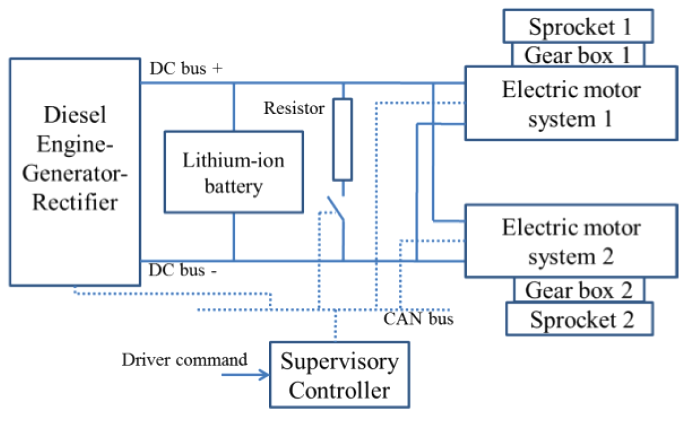
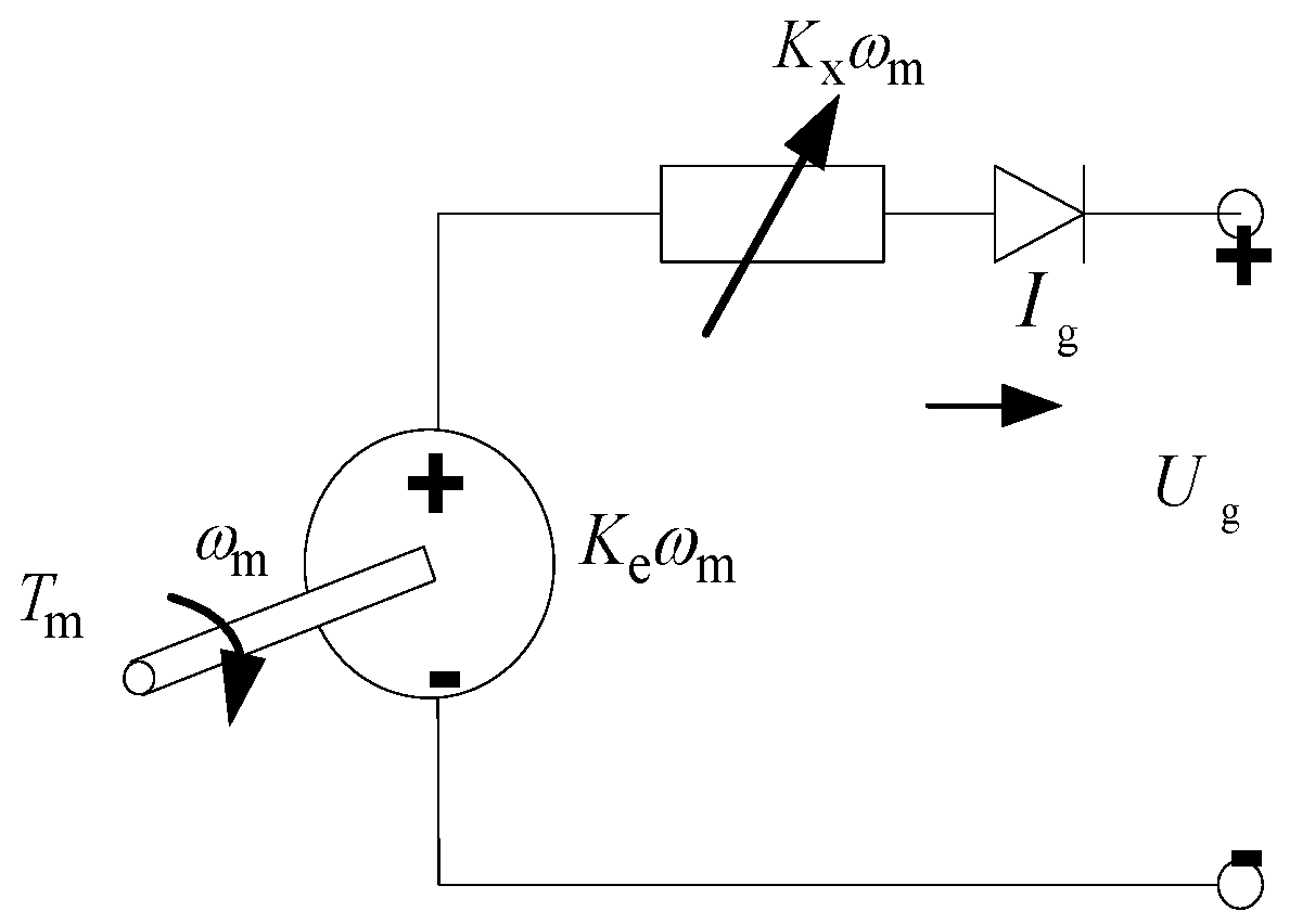
Hybrid propulsion systems for tracked vehicles are being actively pursued, owing to their improved fuel economy, significant on-board electricity supply and stealth operation ability. Some hybrid powertrains have been applied to tracked vehicles, and the engineering and prototype implementation was reported [1,2,3,4]. Compared to hybrid wheeled vehicles, research on hybrid tracked vehicles in an optimization setting is still scanty. Constrained by the component power density and packaging space, a dual-motor drive structure is adopted for a heavy-duty hybrid tracked vehicle, as shown in Figure 1. The two sprockets are separately powered by two electric motors. A diesel engine-generator set and a traction battery pack provide the two motors with electric energy. The vehicle’s drivability like heading or turning is maintained by controlling the speeds/torques of the two motors, while the diesel engine-generator set is controlled to regulate the power distribution between the generator and the battery. This vehicle mostly operates as a serial hybrid, except during the turning, when the outside motor propels and inside one performs braking. The supervisory controller assesses the driver intention and coordinates the work of engine-generator set, battery pack and the two electric motors in an optimal way. Figure 1 also shows a safety design, where a resistor bank is installed and can be switches in case the DC bus voltage exceeds a threshold value.

Figure 1. Dual-motor drive structure of the hybrid tracked vehicle.

Figure 1. Dual-motor drive structure of the hybrid tracked vehicle.

Several studies have focused on the sizing and configuration design to maintain the drivability, and the design of the control strategy for optimal fuel economy [5,6,7,8]. Relatively little work has investigated the parameter sizing and control strategy simultaneously. A general iterative design methodology was used for the optimal design of the plant and controller [9] and it has been applied successfully to the combined automotive suspension and fuel cell optimization [9,10]. In terms of optimal control design, the dynamic programming techniques have been widely applied to wheeled hybrid vehicles and recognized by the academic community for its generic applicability for discrete or continuous state problems with constraints [11,12,13,14]. In this paper, an iterative combined plant-controller optimization methodology is applied to optimize the key parameters of the powertrain and the control strategy simultaneously for a tracked hybrid vehicle. An automatic process iteratively evaluates the fuel consumption as the sizing parameters vary until the combined optimal sizing and control result is obtained.

2. Modeling of Hybrid Electric Powertrains

2.1. Calculation of the Power Requirement for the Engine-Generator and Battery Pack

The tracked vehicle dynamics are mainly based on the work of Bekker’s and Wong’s [15,16]. When only the longitudinal/lateral/yaw motions are considered, the governing equations are:

$$\{\begin{array}{l}{T}_{\text{i}}-(\frac{F_{r\text{i}}r}{i_0\eta }-\frac{M_{r}r}{B{i}_0\eta })=\left[\frac{m{r}^2}{i_0^2\eta }\frac{R}{(R-B/2)}-\frac{I_z{r}^2}{i_0^2\eta B(R-B/2)}\right]{\dot{\omega }}_{\text{i}}\\ T_{\text{o}}-(\frac{F_{r\text{o}}r}{i_0\eta }+\frac{M_{r}r}{B{i}_0\eta })=\left[\frac{m{r}^2}{i_0^2\eta }\frac{R}{(R+B/2)}+\frac{I_z{r}^2}{i_0^2\eta B(R+B/2)}\right]{\dot{\omega }}_{\text{o}}\end{array}$$

(1)

where T_i, T_o are the torques of the inside and outside motors, F_ri, F_ro are the rolling resistance forces of the two tracks, M_r is the resisting yaw moment from the ground, B is the tread of the vehicle, and I_z and m are the yaw moment of inertial and the mass of the vehicle, respectively. r is the radius of the sprocket, i₀ is the fixed gear ratio between motors and sprockets, η is the efficiency from motor shafts to tracks, R is the turning radius of the vehicle, and ω_i, ω_o are the rotational speeds of the inside and outside sprockets, respectively.

Considering a steady-state turning, the resisting yaw moment from the ground is calculated by Equation (2) [16]:

$$M_{\text{r}}=\frac{{\mu }_{\text{t}}mgl}{4}$$

(2)

where µ_t is the coefficient of the lateral resistance, g is 9.81 m/s², and l is the contact length of the track.

Based on empirical results, µ_t was found to be [17]:

$${\mu }_{\text{t}}={\mu }_{\max }\cdot {(0.925+0.15\cdot R/B)}^{-1}$$

(3)

where µ_max is the maximum value of the coefficient of lateral resistance, which is dependent on terrain type. The rolling resistant forces acting on the two tracks are:

$$F_{r\text{i}}=F_{r\text{o}}=0.5\cdot f_{\text{r}}\cdot mg$$

(4)

where f_r is the coefficient of motion resistance of the vehicle in the longitudinal direction.

When the track slip/skid is omitted the turning radius R can be calculated from Equation (5):

$$R=\frac{B}{2}\frac{{\omega }_{\text{o}}+{\omega }_{\text{i}}}{{\omega }_{\text{o}}-{\omega }_{\text{i}}}$$

(5)

The rotational speeds of the outside and inside sprockets, ω_o and ω_i, can be calculated from:

$${\omega }_{\text{o,i}}=\frac{30\cdot v_{\text{o,i}}\cdot i_0}{\pi \cdot r}$$

(6)

where v_o,i are the speeds of the two tracks. Like in Equation (5), an implied assumption of Equation (6) is also that the track slippage is ignored.

The electric power P_req requested by the two motors varies as the driving mode changes, especially during braking. Two kinds of electric braking are adopted to reduce mechanical friction brake: resistor braking and regenerative braking. To recuperate the braking energy as much as possible, regenerative braking is applied prior to resistor braking. However, resistor-braking is used if the DC bus voltage U_dc is higher than a threshold value U_thr for safe operation of the electronic devices. The value of P_req is calculated from Equation (7), where P_req is positive when the electric power outputs and negative when the electric power is recuperated in regenerative braking. It must be noted that in this vehicle, the regenerative braking only happens when U_dc < U_thr; otherwise the resistor braking is triggered, and the electric power will be consumed by resistor-heating. In that case, P_req remains positive whenever the electric motors drive or brake:

$$P_{\text{req}}=\{\begin{array}{l}{T}_{\text{o}}{\omega }_{\text{o}}{\eta }_{\text{mot}}^{-\text{sgn}(T_1)}+T_{\text{i}}{\omega }_{\text{i}}{\eta }_{\text{mot}}^{-\text{sgn}(T_2)}{U}_{\text{dc}}\text{<}{U}_{\text{thr}}\\ \left|T_{\text{o}}{\omega }_{\text{o}}{\eta }_{\text{mot}}^{-\text{sgn}(T_1)}\right|+\left|T_{\text{i}}{\omega }_{\text{i}}{\eta }_{\text{mot}}^{-\text{sgn}(T_1)}\right|U_{\text{dc}}\ge U_{\text{thr}}\end{array}$$

(7)

Field experiments were conducted to collect test speed data to be used as the driving schedule for the sizing and control design, shown in Figure 2. It included significant accelerations, braking and steering. The maximum and average vehicle speeds and the travel distance are 36 km/h, 14.43 km/h, and 3.976 km, respectively.

Figure 2. The speed profile used as the driving cycle for the tracked vehicle studied.

Figure 2. The speed profile used as the driving cycle for the tracked vehicle studied.

2.2. The Diesel Engine-Generator and Battery Model

The diesel engine, permanent magnetic AC generator, and three-phase full wave rectifier are simplified as the electric circuit shown in Figure 3, where T_m is the motor torque, ω_m is the rotational speed, K_e is the coefficient of the electromotive force, K_xω_m is the electromotive force, which increases proportionally to ω_m, in which K_x = 3PL^g/π. P is the number of poles and L^g is the synchronous inductance of the armature.

Figure 3. The simplified generator-rectifier equivalent circuit.

Figure 3. The simplified generator-rectifier equivalent circuit.

The variable I_g is the electric current from the generator and U_g is the output voltage. The water-cooled 6-cylinder V-engine with a fully electronically controlled injection and a turbocharger gives the maximum torque of 1940 Nm around the rotational speed of 1300 rpm and reaches the maximum power output at the permitted maximum rotational speed of 2000 rpm.

The dynamics of the generator-rectifier is described by Equations (8)–(11):

$$\frac{T_{\text{eng}}}{i_{\text{e}-\text{g}}}-T_{\text{m}}=0.1047(\frac{J_{\text{e}}}{i_{\text{e}-\text{g}}^2}+J_{\text{g}})\frac{d{n}_{\text{g}}}{dt}$$

(8)

$$T_{\text{m}}=K_{\text{e}}{I}_{\text{g}}-K_{\text{x}}{I}_{\text{g}}^2$$

(9)

$$U_{\text{g}}=K_{\text{e}}{\omega }_{\text{m}}-K_{\text{x}}{\omega }_{\text{m}}{I}_{\text{g}}$$

(10)

$$n_{\text{g}}=i_{\text{e}-\text{g}}{n}_{\text{eng}}$$

(11)

where i_e-g is the fixed gear ratio between the engine and the generator, n_eng and n_g are the rotational speeds of the engine and generator, respectively, and J_e and J_g are the moment of inertia of the engine and the generator. Engine torque T_eng is regulated to control the power distribution between the generator and the battery pack. The test and the simulated results are shown in Figure 4. It can be seen that U_g and n_eng are predicted accurately by the model.

Figure 4. Simulation vs. experiment results of the voltage and speed history during the dynamic load.

Figure 4. Simulation vs. experiment results of the voltage and speed history during the dynamic load.

The lithium-ion battery pack is described by the following simple internal resistance model:

$$\{\begin{array}{l}{U}_{\text{bat}}=\{\begin{array}{l}V(\text{SOC})-I_{\text{bat}}\cdot R_{\mathrm{int}\_\text{ch}}(\text{SOC})\text{ (}{I}_{bat}>0)\\ V(\text{SOC})-I_{\text{bat}}\cdot R_{\mathrm{int}\_\text{dis}}(\text{SOC})\text{ (}{I}_{bat}<0)\end{array}\\ \text{SOC}=(\text{1}-\frac{\text{1}}{3600C}{\displaystyle \int I_{\text{bat}}dt)\times 100\%}\end{array}$$

(12)

where U_bat is the battery output voltage, V(SOC) is the open circuit voltage, I_bat is the battery current, R_{int_ch}(SOC) and R_{int_dis}(SOC) are the internal resistance during charging and discharging, respectively, and C is the capacity of the battery. The values of V(SOC), R_{int_ch}(SOC) and R_{int_dis}(SOC) vary as SOC changes and are obtained through experiments, as shown in Figure 5.

Figure 5. Battery open-circuit voltage and internal resistance obtained through experiments.

Figure 5. Battery open-circuit voltage and internal resistance obtained through experiments.

For the tracked vehicle, stealth operation is an advantage and desired feature through reduced thermal and acoustic signatures. In order to maintain this operating mode, the energy stored in the battery pack should be kept within a reasonable range. In particular, Equation (13) is suggested:

$$V(0.7)\cdot C\ge E_{\text{ele}}$$

(13)

where E_ele is the energy value necessary to support a specified stealthy mode operation range, obtained through tests at different discharge rate.

In addition, Equation (14) must be satisfied at all time to maintain the drivability in the driving schedule:

$$P_{\text{req}}=U_{\text{dc}}(I_{\text{g}}+I_{\text{bat}})$$

(14)

where the value of U_dc is determined by:

$$U_{\text{dc}}=\{\begin{array}{l}{U}_{\text{bat}}\text{ > }{U}_{\text{g}}\text{, }{I}_{\text{g}}\text{ = 0}\\ U_{\text{g}}\text{ = }{U}_{\text{bat}}\text{, }{I}_{\text{g}}\text{ > 0}\end{array}$$

(15)

where I_g = 0 occurs when U_g is lower than U_bat and thus the generator is not producing any electric power. In this case the battery pack will supply all the power. The values of the vehicle’s key parameters are summarized in Table 1 below.

Table 1. Values of the vehicle’s key parameters.

Parameters. Unit	m [kg]	Iz [kgm2]	i0	r [m]	B [m]	Ke [V s rad−2]	Kx [N m A−2]	ie-g	C [Ah]	Je [kgm2]	Jg [kgm2]	l [m]
Value	15,200	55,000	13.2	0.313	2.55	1.65	0.00037	1.60	50	3.2	2.0	3.57

Table 1. Values of the vehicle’s key parameters.

Parameters. Unit	m [kg]	Iz [kgm2]	i0	r [m]	B [m]	Ke [V s rad−2]	Kx [N m A−2]	ie-g	C [Ah]	Je [kgm2]	Jg [kgm2]	l [m]
Value	15,200	55,000	13.2	0.313	2.55	1.65	0.00037	1.60	50	3.2	2.0	3.57

Equations (1)–(15) describe the dynamics of the hybrid tracked vehicles. Given the typical driving schedule and the component parameters, T_eng should be regulated in an optimal way to determine the power distribution between the generator set and the battery pack to achieve minimum fuel consumption. Here the electronic accelerator pedal signal Acc_eng is normalized between [0, 1] to regulate T_eng within the admissible range.

3. DP-Based Strategy and Optimization

Equations (1)–(15) are discretized to formulate into a DP problem. The time step T_s is set to 0.1 s considering the balance between computation cost and accuracy. The optimal control Acc_eng(k) (k = 0, 1, …, N − 1) is pursued to minimize the total fuel consumption during the given driving schedule as follows:

$$J(x(0))={\displaystyle \sum _{i=0}^{N-1}{T}_{\text{s}}\cdot F(n_{eng}(k),T_{eng}(k))}$$

(16)

subject to the following constraints:

$$x(k+1)=f(x(k),Ac{c}_{\text{eng}}(k),P_{\text{req}}(k\left)\right)$$

(17)

$$|\text{SOC}(N)-\text{SOC}(0)|<\Delta \text{SOC}$$

(18)

$$n_{eng\_idle}<n_{eng}(k)<n_{eng\_\max }$$

(19)

$$\left|n_{eng}(k+1)-n_{eng}(k)\right|<\Delta n$$

(20)

$$I_{bat\_\max \_char}<I_{bat}(k)<I_{bat\_\max \_disch}$$

(21)

$$0<I_g(k)<I_{g\_\max }$$

(22)

In Equations (16)–(22), F is the fuel consumption rate determined by n_eng(k) and T_eng(k), normally obtained through a fuel consumption table derived through bench tests. x(k) = [SOC(k), n_eng(k)], and f represents the discrete dynamics from Equations (1)–(15). The increment of n_eng is also constrained to emulate the dynamics of the engine. Typically, the HEV control strategy requests the energy balance for the battery pack at the end of the driving schedule, and SOC(N) is hence enforced to equal the initial value.

The DP technique is applied to solve the above problem based on the principle of optimality, which is expressed as:

$$J(x(k))=\underset{Ac{c}_{eng}(k)}{\min }\{J(x(k+1))+T{\cdot }_{\text{s}}F(n_{eng}(k),T_{eng}(k))\}$$

(23)

where J(x(k)) is the optimal cost function at state (x(k) starting from step k. When (x(k) and Acc_eng(k) are discretized into the finite states and Equation (23) is solved backwards, the optimal control and corresponding cost are stored and then the optimal solution with the specific initial states is retrieved forwardly by applying the optimal controls through the horizon.

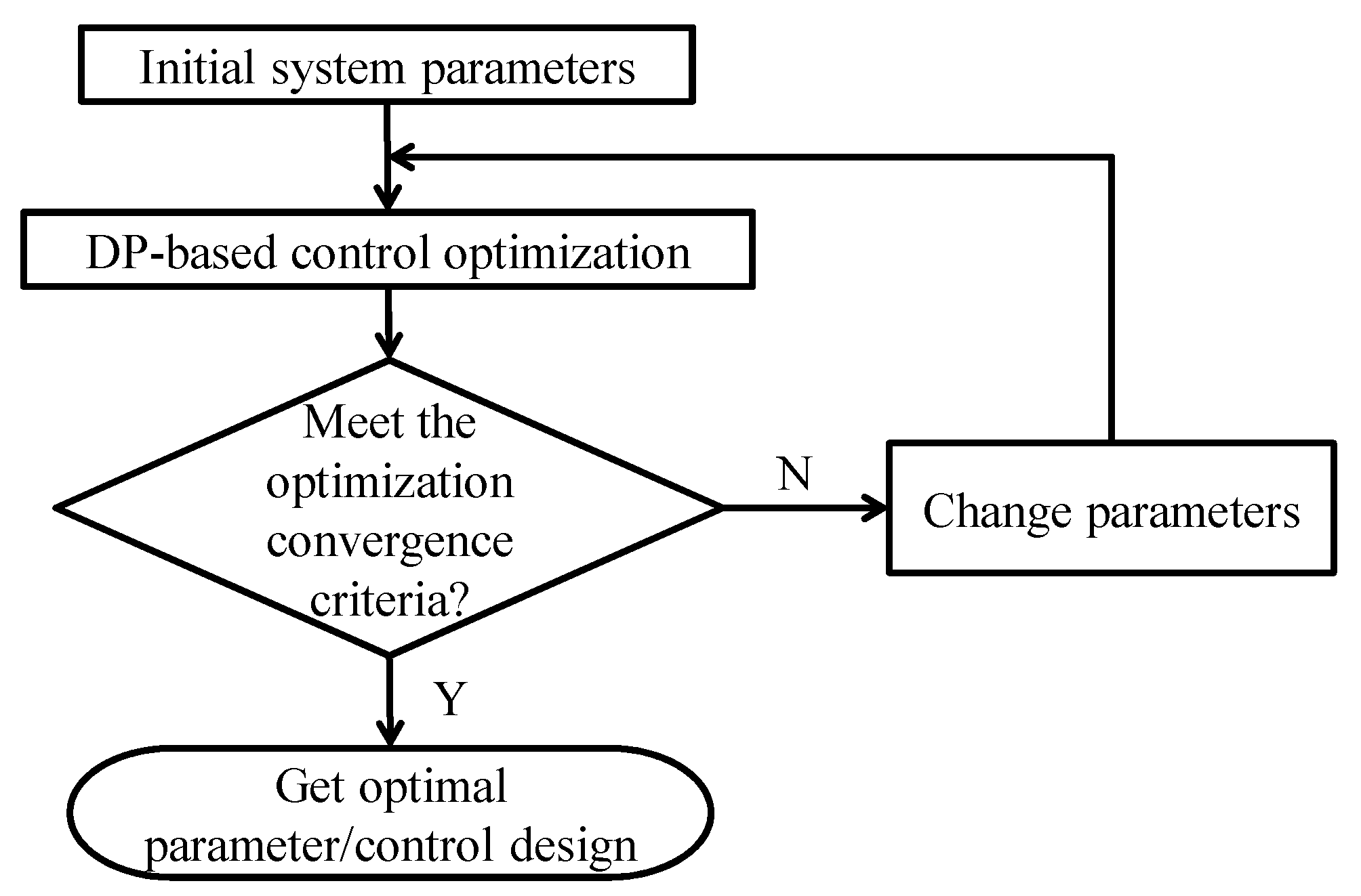
The control rule can be extracted from the DP results, as a casual control strategy. However, since some important parameters couple closely with the control, and the DP-based control strategy is just optimal given the particular system parameters, the following combined optimization of the system parameters and control strategy in the synergic way is significant.

4. Combined Optimization Problem Formulation

4.1. Combined Optimization Framework

Given the vehicle system parameters, DP can be used to find the optimal control under constraints for a specific driving schedule. When the system parameters vary in the feasible range and DP is applied iteratively, the optimal combination of the parameters and control will be identified. Four kinds of combined optimization methods were observed by Fathy et al. [9]. In this paper the Bi-level combined plant/controller optimization is adopted, consisting of two nested optimization loops. The outer loop optimizes the fuel consumption by only changing the system parameters. The inner loop generates the optimal control strategy for the parameters selected by the outer loop. These two loops form the integrated plant/controller optimization, which generates the global optimal design for the system parameters and control strategy. The Bi-level combined optimization process is shown in Figure 6.

Figure 6. Bi-level combined optimization process.

Figure 6. Bi-level combined optimization process.

4.2. The Scaled Model and Optimization Problem Formulation

The scaled models are needed to parameterize the system conveniently during the optimization process. In this paper the engine sizing is fixed and the battery capacity and open circuit voltage is scaled by the scale factors x_CAP and x_OCV, respectively. Here the internal resistance is assumed to be proportional to the open circuit voltage and inversely proportional to the capacity. The battery capacity, open circuit voltage and internal resistance are calculated by Equations (24)–(27):

$$C=x_{\text{CAP}}\cdot C_{\text{bas}}$$

(24)

$$V(\text{SOC})=x_{\text{OCV}}\cdot V_{\text{bas}}(\text{SOC})$$

(25)

$$R_{\mathrm{int}\_\text{ch}}(\text{SOC})=x_{\text{ocv}}/x_{\text{cap}}\cdot R_{\mathrm{int}\_\text{ch\_bas}}(\text{SOC})$$

(26)

$$R_{\mathrm{int}\_\text{dis}}(\text{SOC})=x_{\text{ocv}}/x_{\text{cap}}\cdot R_{\text{int\_dis\_bas}}(\text{SOC})$$

(27)

where C_bas is the baseline capacity, V_bas(SOC) is the baseline open circuit voltage of the battery pack varying as a function of SOC. R_{int_ch_bas}(SOC), R_{int_dis_bas}(SOC) is the baseline internal resistor varying with SOC.

Because the gear ratio i_e-g between the diesel engine and the generator plays an important role in scaling the engine’s speed/torque into the generator’s range, it is also selected as a parameter to be optimized in the outer loop. The degree of hybridization is adopted to measure the relative power size of the primary power source and the secondary power source. In the serial hybrid configuration for this tracked vehicle, the diesel engine-generator is the primary power source and the battery pack is the secondary power source. To avoid optimal but unphysical solutions, the degree of hybridization is constrained to [0, 0.4] and calculated by Equation (28):

$$x_{\text{h}}\text{=}{P}_{\text{bat\_max}}/(P_{\text{bat\_max}}\text{+}{P}_{\text{gen\_max}}\text{)}$$

(28)

where P_{bat_max} is the maximum power battery pack outputs, and P_{gen_max} is the maximum power the generator provides. The value of P_{bat_max} is calculated based on the practical current range as defined by Equation (29):

$$P_{\text{bat\_max}}=\underset{\text{SOC}\in \text{[0,1]}}{\max }\frac{V^2(\text{SOC})}{4\cdot R_{\text{int\_dis}}(\text{SOC})}$$

(29)

The combined optimal problem is formulated with all the feasible constraints:

$$\underset{x_{\text{OCV}},x_{\text{CAP}},i_{\text{e-g}},x_{\text{h}}}{\min }\left\{{\displaystyle \sum _{i=0}^{N-1}{T}_{\text{s}}\cdot F(n_{\text{eng}}(k),T_{\text{eng}}(k))}\right\}$$

(30)

subject to:

$$\begin{array}{l}x(k+1)=f(x(k),Ac{c}_{\text{eng}}(k),P_{\text{req}}(k\left)\right)\\ 0.2\le x_{\text{OCV}}\le 2\\ x_{\text{h}}\le 0.4\\ 0.2\le x_{\text{CAP}}\le 2\\ 1\le i_{\text{e-g}}\le 4\\ V(0.7)\cdot C<E_{\text{ele}}\\ |\text{SOC}(N)-\text{SOC}(0)|<\Delta \text{SOC}\\ n_{eng\_idle}<n_{eng}(k)<n_{eng\_\max }\\ \left|n_{eng}(k+1)-n_{eng}(k)\right|<\Delta n\\ I_{bat\_\max \_char}<I_{bat}(k)<I_{bat\_\max \_disch}\\ 0<I_g(k)<I_{g\_\max }\end{array}$$

(31)

where x_ocv, x_cap, x_h, i_e-g,n_eng, I_bat, and I_g are constrained to their respective feasible ranges. The product of the open circuit voltage when SOC = 0.7 and the capacity should be more than the energy value supporting the sufficient stealthy operation range. Notice that ACC_eng(k) incorporated in Equation (30) influences T_eng(k) directly and is determined in the inner loop by DP method.

5. Results and Discussion

The combined optimization is computationally expensive due to the dual-loop iterative process. In order to improve the computational efficiency, once the constraint in the inner loop is violated the current exploitation stops and the cost is set to a large infeasible value. A strong nonlinearity is observed and the data shown in the map is a bit noisy. The DOE (Design of Experiments) technique is first applied to explore the response map in all the feasible design spaces based on Latin Hypercube sampling and then the Non-linear Programming by Quadratic Lagrangian (NLPQL) algorithm is applied to obtain the global optimal value [18].

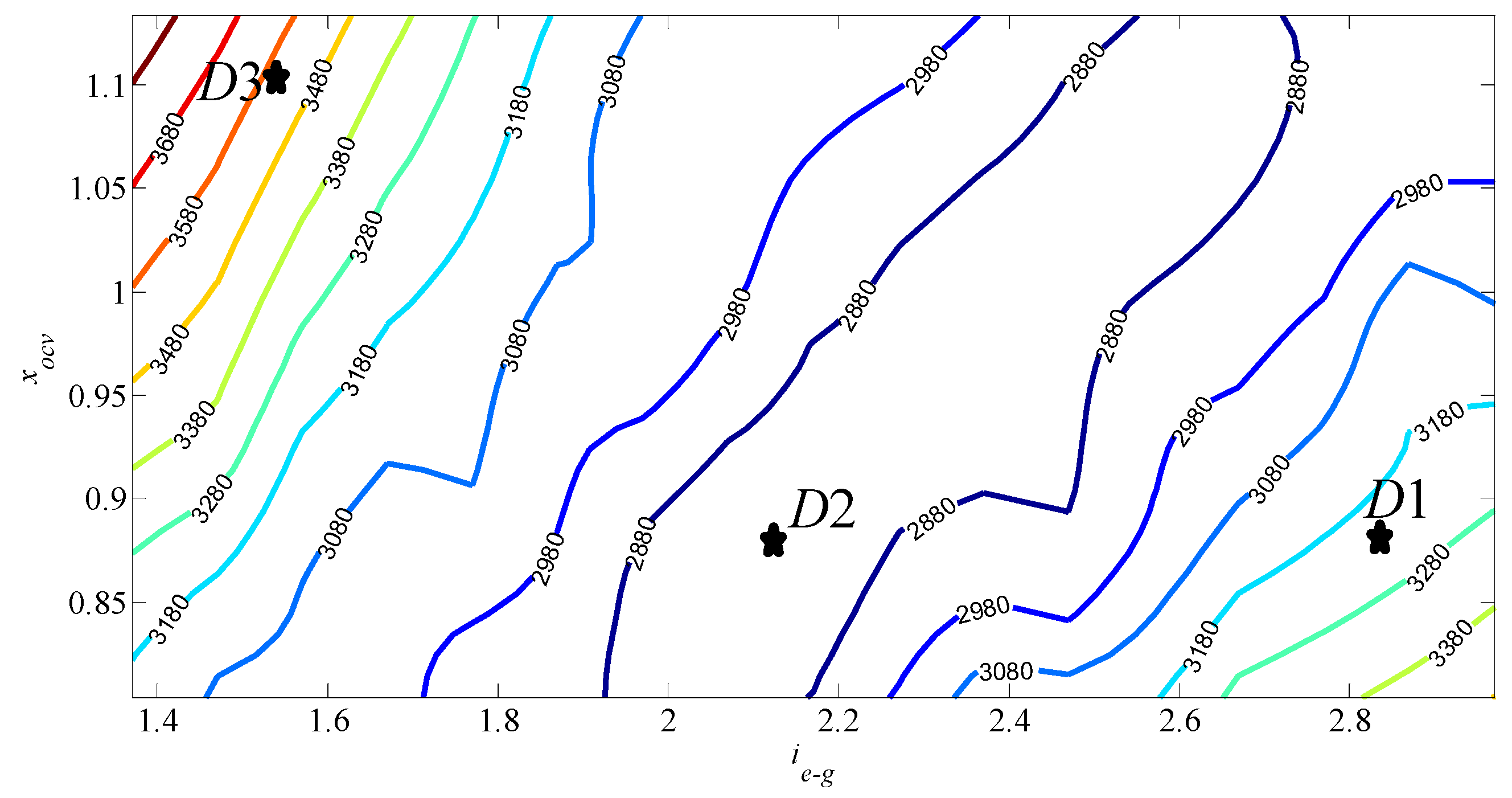
The relationship of the fuel consumption, i_e-g and x_ocv is shown in Figure 7, in which the optimal correspondence between i_e-g and x_ocv is observed explicitly. This means that i_e-g increases or decreases with x_ocv to maintain an optimal fuel economy. Further investigation shows that the voltage range of the battery pack and the engine-generator match well to make the optimal power distribution between them possible. It may thus be concluded that the energy distribution control has a limited influence on the fuel economy without the proper match between i_e-g and the voltage range of the battery pack. The proper match is necessary to keep a good fuel economy. It should be noted that the optimal power distribution control plays a valuable role if i_e-g and the voltage range of the battery is constrained to the optimal area shown in Figure 7, which allows the component sizing or parameter to be freely selected. 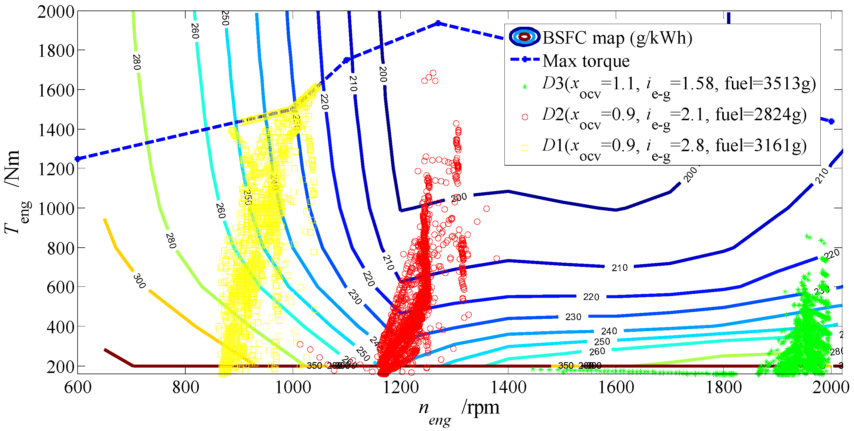Figure 8 shows the engine working points under the optimal control when i_e-g and x_ocv are selected differently. It can be seen that the engine works near the high efficiency area if i_e-g and x_ocv match well, just as the parameter selection D2 in Figure 8, with a lower fuel consumption of 2824 grams. Otherwise the engine works far from the high efficiency area, just like the parameter selections D1 or D3 with 3163 and 3513 grams, 12.0% and 24.4% higher than that of D1, respectively.

Figure 7. The fuel consumption contour (grams) vs. i_e-g and x_ocv.

Figure 7. The fuel consumption contour (grams) vs. i_e-g and x_ocv.

Figure 8. Engine operating points in three different parameter selection (x_cap = 2, x_h < 0.4).

Figure 8. Engine operating points in three different parameter selection (x_cap = 2, x_h < 0.4).

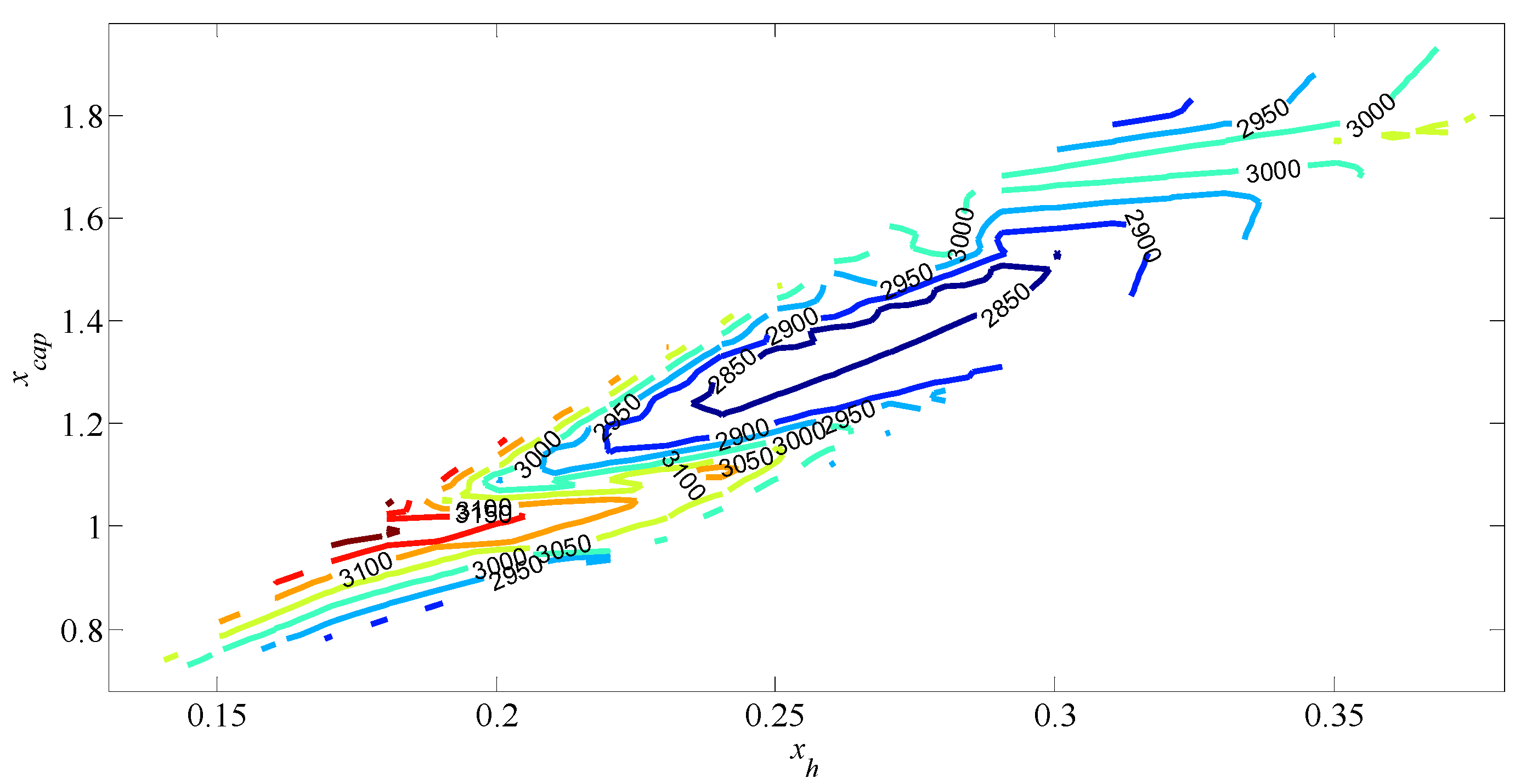
The relationship of the fuel consumption, x_cap and x_h is shown in Figure 9. The values of x_h and x_cap must remain in a specific range to obtain the optimal fuel economy. Although this map is a bit noisy, there is an optimal range [0.25, 0.32] for x_h. This fact allows us to conclude that in such a kind of hybrid vehicle, x_h should be selected with great caution because the fuel economy does not always increase as x_h increases. There is a more sophisticated interaction between the fuel consumption, x_h and x_cap.

Figure 9. Fuel consumption vs. x_cap and x_h.

Figure 9. Fuel consumption vs. x_cap and x_h.

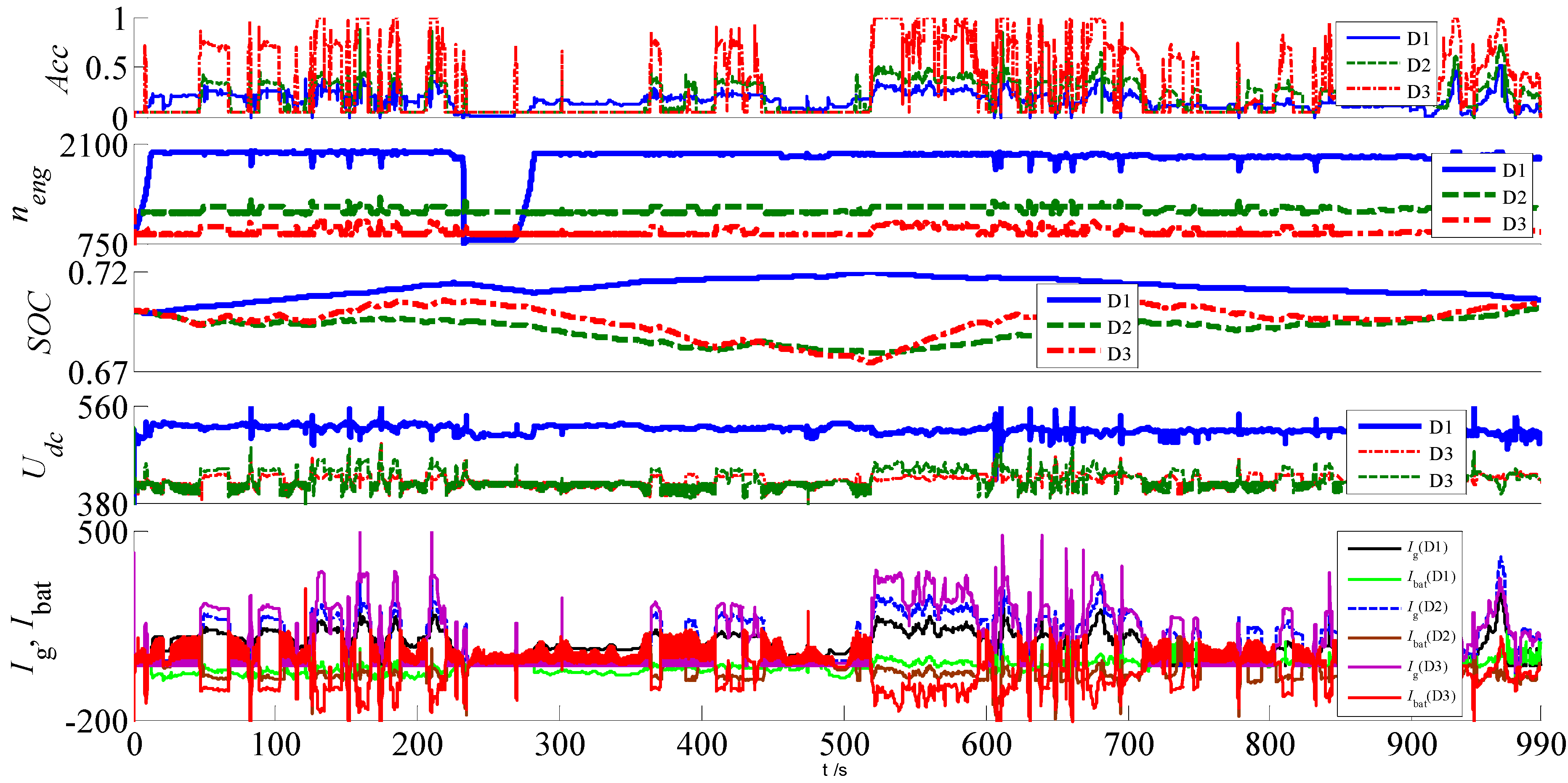
The dynamic evolutions of the system with the parameter selection D1, D2, D3 are shown in Figure 10. D1 and D3 represent two type mismatches of the engine-generator and the battery. The value of i_e-g is too higher than the voltage range of the battery in D1, and vice versa in D3.

Figure 10. Dynamic history of typical variables in D1, D2, D3.

Figure 10. Dynamic history of typical variables in D1, D2, D3.

The engine speed is constrained to the undesirable range in D1 and D3. Clearly, DP finds the different controls for the different parameter selections. For D1, the engine always operates in the high speed range to generate electricity, while the engine is idled when the power request is low during around 230–260 s. For D1 and D2, the engine works around 900 rpm and 1200 rpm, respectively. The engine frequently generates maximum torque to increase its power output in D1 due to its low speed range. D2 has the relative proper torque and speed output and achieves the lowest fuel consumption. It is clear that the battery tends to be charged or discharged at higher current in D3 than in D2, and it is used less frequently in D1 than in D2. This observation is also useful for the proper battery parameter design. This may lead to the conclusion that the voltage match between the generator at the desired speed range and the battery at admission SOC range is very important. A good match will guarantee the battery can supply the electric power properly, avoiding overuse and insufficient participation.

The optimized and initial parameters are shown in Table 2, where i_e-g, the battery capacity and the voltage range are solved simultaneously to obtain the results shown in Figure 8 and Figure 9. It should be noted the battery capacity increases by 28.0%, and the voltage decreases to 89.9% of the original level. This helps improve the ability to supply the bigger transient electric current without any significant loss of the battery reliability. A considerable reduction of fuel consumption is achieved, namely 16.2% lower than the fuel consumption under the initial parameters.

Table 2. The combined optimal design vs. the initial design.

Optimal design results							Initial design values				Fuel economy Improvement
x*ocv	x*cap	x*h	i*e-g	c* [Ah]	V*(1) [V]	Fuel consumption* [grams]	C [Ah]	V(1) [V]	ie-g	Fuel consumption [grams]
0.90	1.68	0.25	2.15	64	436	2820	50	485	1.60	3365	16.2%

Table 2. The combined optimal design vs. the initial design.

Optimal design results							Initial design values				Fuel economy Improvement
x*ocv	x*cap	x*h	i*e-g	c* [Ah]	V*(1) [V]	Fuel consumption* [grams]	C [Ah]	V(1) [V]	ie-g	Fuel consumption [grams]
0.90	1.68	0.25	2.15	64	436	2820	50	485	1.60	3365	16.2%

Clearly in this hybrid tracked vehicle the parameter selection plays a significant role in the optimal system design and the proper parameter match is a necessary prerequisite for a good fuel economy, especially for some predominant parameters, such as the battery voltage and the generator speed which are influenced heavily by the gear-ratio between the engine and generator. The mismatch results in the limited improvement in fuel economy even through the control optimization. It should also be noted that the fuel economy obtained in the paper is the theoretically best with respect to the current parameter selection and the optimal control. The casual control algorithm approximating DP behavior should be pursued in the following practical controller design, which is not covered in the paper.

6. Conclusions

The combined optimization of the sizing and power distribution control for a hybrid tracked vehicle is investigated in this paper. The hybrid electric powertrains are first modeled and verified through test results. The Dynamic Programming technique is applied to find the optimal control given the driving schedule from the field test and particular system parameters. A comprehensive Bi-level optimization framework suitable for the above problem is presented and applied to optimize the parameter sizing and control iteratively. The optimal results are analyzed to disclose the interaction between sizing and control design, which is helpful for the combined system sizing and control design in a synergic way. It clarifies that both the parameter sizing and control optimal design are important equally for the hybrid propulsion of the tracked vehicle. The sizing defines the optimal possibility of the components’ collaborations, and the optimal control identifies the solution matching the sizing and realizes that possibility. The parameter selection without the consideration of the optimal control implementation in the later phase is difficult to maintain the combined optimal design. A significant reduction of the fuel consumption is observed. The combined methodology proposed in the paper is instructive to other hybrid propulsion designs. It also should be noted that the large amount of driving schedules involved help find and improve the combined optimal design.