Optimal Bidding Strategies for Wind Power Producers in the Day-ahead Electricity Market


Abstract
:
1. Introduction
2. Problem Description
2.1. Market Framework
2.2. Profit of Wind Power Producers
3. Mathematical Formulation
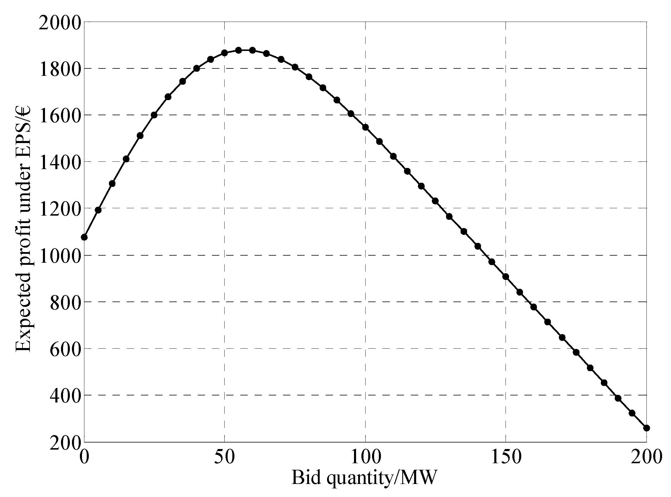
3.1. Expected Profit-Maximization Bidding Strategy
3.2. Chance-Constrained Programming-Based Bidding Strategy
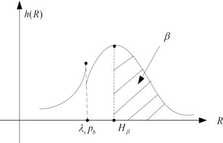
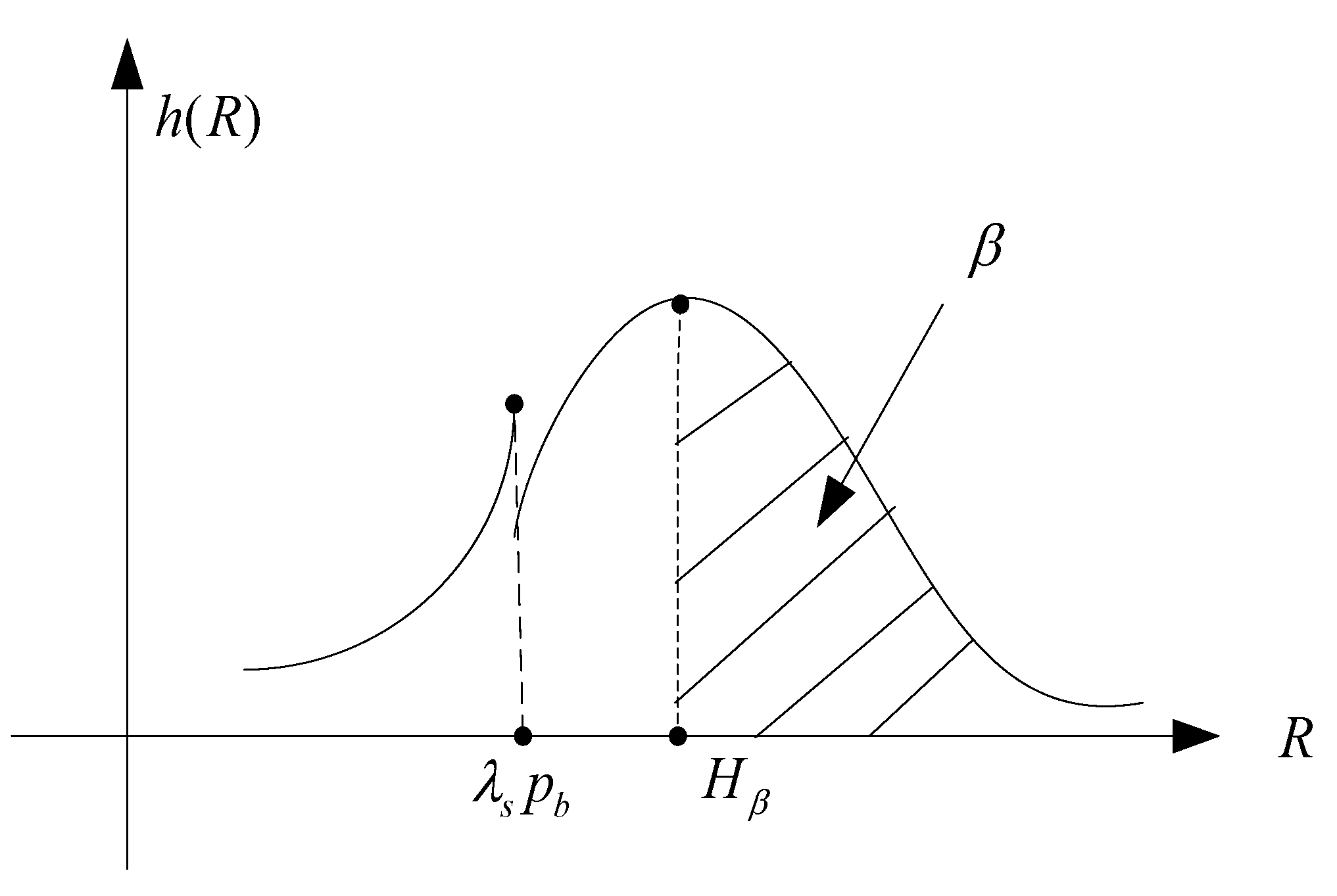
3.2.1. Cumulative Distribution of Random Variable R

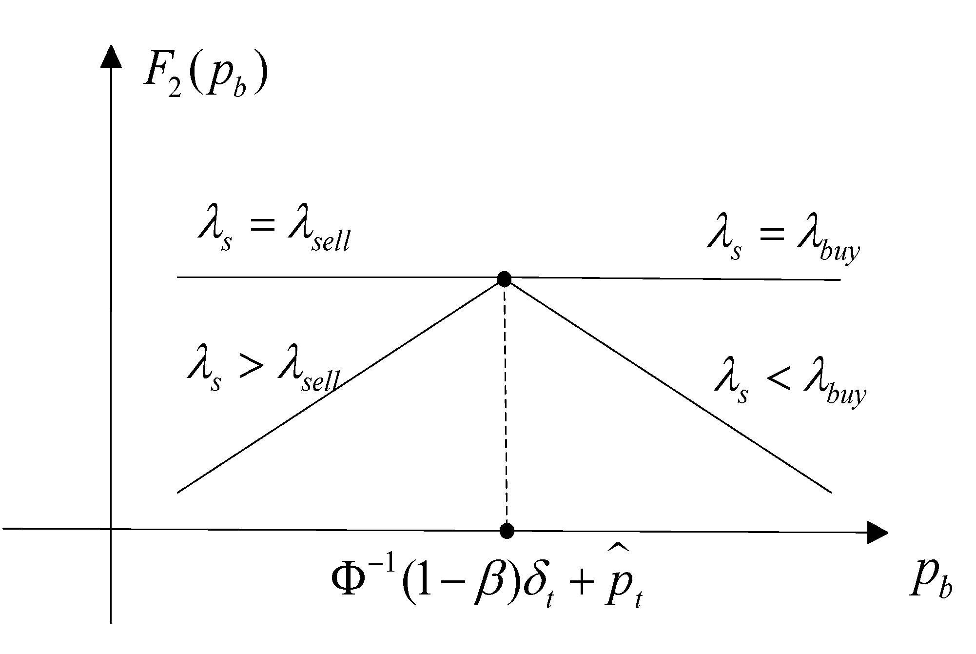
3.2.2. Formulation of the CPS


| Range of β | Relationship among λs, λsell and λbuy | Optimal solution, | F2() |
|---|---|---|---|
| 0 | |||
3.3. Multi-Objective Bidding Strategy
3.3.1. Multi-Objective Bidding Model
3.3.2. Solution of Multi-objective Bidding Model
- Case (1a) if λsell ≤ λs < αλbuy + (1 − α)λsell, we have dg1(pb)/dpb < 0, the function G1(pb) is monotonically decreasing, we get = 0, and = G1(0).
- Case (1b) if αλbuy + (1 − α)λsell ≤ λs ≤ λbuy, from, dg1(pb)/dpb = 0, we have , and 0 ≤ z1 ≤1, the extreme point pb = Φ−1(z1)δt + μt. Three cases are considered further:
- if Φ−1(z1)δt + μt < 0, = 0, = G1(0);
- if 0 ≤ Φ−1(z1)δt + μt ≤ pmax, = Φ−1(z1)δt + μt, = G1(Φ−1(z1)δt + μt);
- if Φ−1(z1)δt + μt > pmax, = pmax, = G1(pmax).
- Case (2a) if (1 − α)λbuy + αλsell) ≤ λs ≤ λbuy, dg1(pb)/dpb > 0, the objective function is monotonically decreasing, we get = pmax, = G2(pmax).
- Case (2b) if λsell ≤ λs ≤ (1 − α)λbuy + αλsell, from dg2(pb)/dpb = 0, we have , and 0 ≤ z2 ≤ 1. Three cases are considered further:
- if Φ−1(z2)δt + μt < 0, = 0, = G2(0);
- if 0 ≤ Φ−1(z2)δt + μt ≤ pmax, = Φ−1(z2)δt + μt, = G2(Φ−1(z2)δt + μt);
- if Φ−1(z2)δt + μt > pmax, = pmax and = G2(pmax).
- Case (3a) 0 ≤ pb ≤ Φ−1(1 − β)δt + μtIn this case, we apply model (23), and then two more cases are considered:
- (i)
- if (1 − α)λbuy + αλsell ≤ λs ≤ λbuy, the optimal bid is = Φ−1(1 − β)δt + μt, and = G2(Φ−1(1 − β)δt + μt);
- (ii)
- if λsell ≤ λs ≤ (1 − α)λbuy + αλsell. Three cases are considered further:if Φ−1(z2)δt + μt < 0, = 0, = G2(0);if 0 ≤ Φ−1(z2)δt + μt ≤ Φ−1(1 − β)δt + μt, = Φ−1(z2)δt + μt and = G2(Φ−1(z2)δt + μt);if Φ−1(z2)δt + μt > Φ−1(1 − β)δt + μt, = Φ−1(1 − β)δt + μt and = G2(Φ−1(1 − β)δt + μt).
- Case (3b) Φ−1(1 − β)δt + μt ≤ pb ≤ pmaxIn this case, we apply the model (22). Similarly, as in Case (3a),
- (i)
- if λsell ≤ λs < αλbuy + (1 − α)λsell, the optimal bid is = Φ−1(1 − β)δt + μt, and = G1(Φ−1(1 − β)δt + μt).
- (ii)
- if αλbuy + (1 − α)λsell ≤ λs ≤ λbuy. Three cases are considered further:if Φ−1(z1)δt + μt < Φ−1(1 − β)δt + μt, = Φ−1(1 − β)δt + μt, = G1(Φ−1(1 − β)δt + μt);if Φ−1(1 − β)δt + μt ≤ Φ−1(z1)δt + μt ≤ pmax, = Φ−1(z1)δt + μt and = G1(Φ−1(z1)δt + μt);if Φ−1(z1)δt + μt > pmax, = pmax, and = G1(pmax).
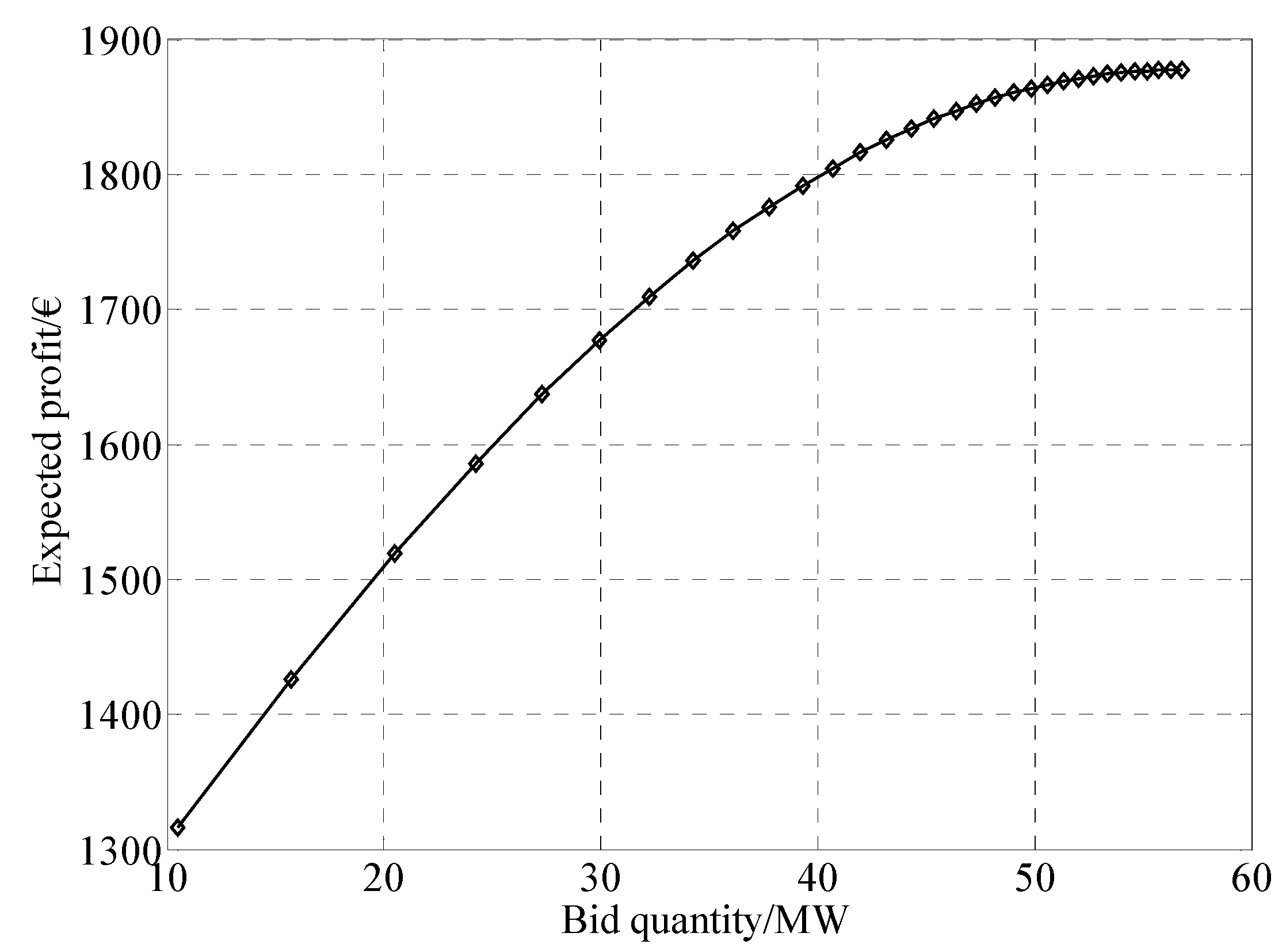
3.3.3. Best Compromise Solution
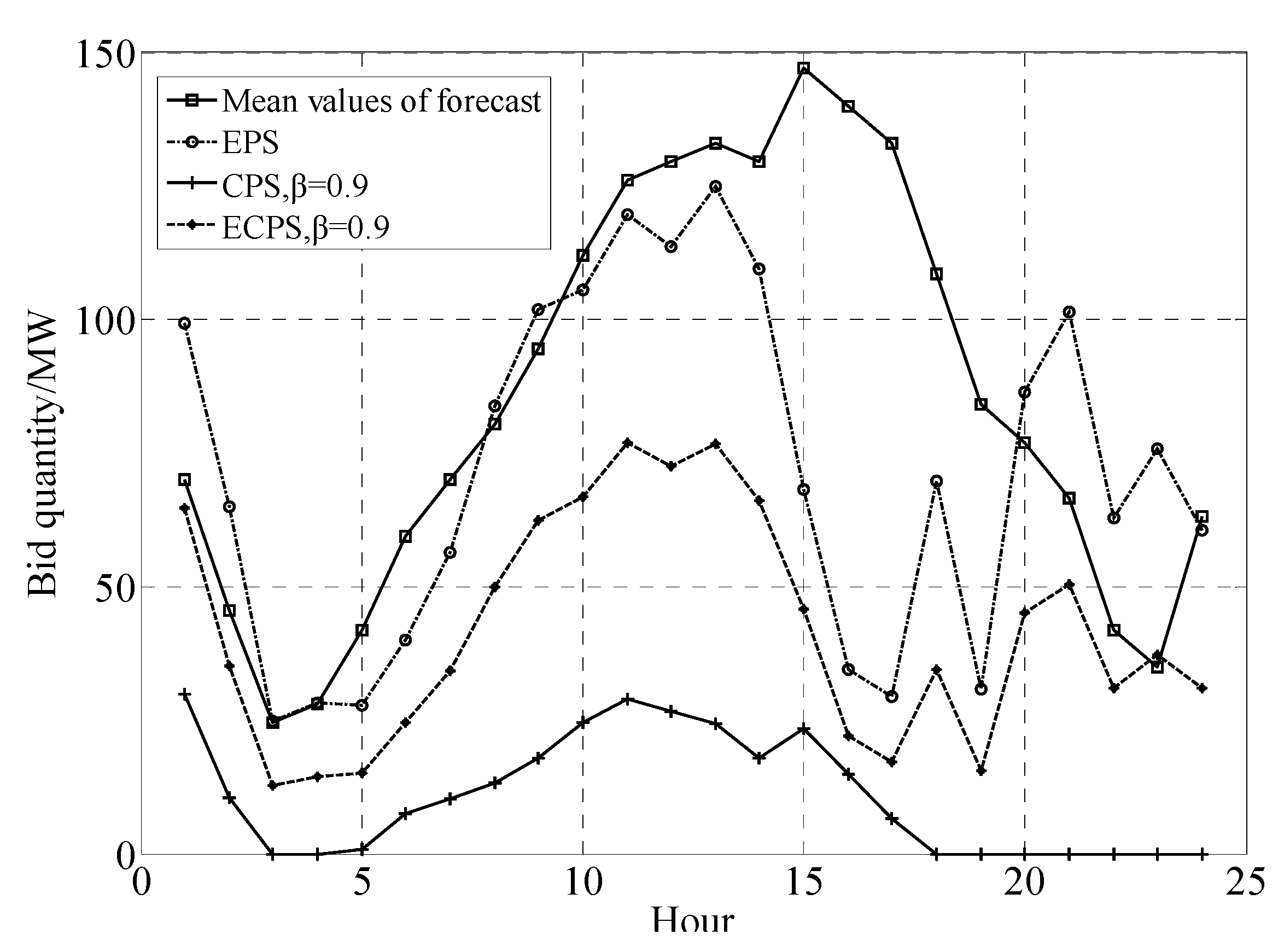
4. Numerical Simulation
| Hour | Expected value/MW | Standard deviation/MW | Hour | Expected value/MW | Standard deviation/MW |
|---|---|---|---|---|---|
| 1 | 70.0 | 31.37 | 13 | 133.0 | 84.76 |
| 2 | 45.5 | 27.32 | 14 | 129.5 | 87.06 |
| 3 | 24.5 | 21.53 | 15 | 147.0 | 96.39 |
| 4 | 28.0 | 24.61 | 16 | 140.0 | 97.62 |
| 5 | 42.0 | 32.08 | 17 | 133.0 | 98.6 |
| 6 | 59.5 | 40.5 | 18 | 108.5 | 92.18 |
| 7 | 70.0 | 46.63 | 19 | 84.0 | 83.86 |
| 8 | 80.5 | 52.49 | 20 | 77.0 | 82.92 |
| 9 | 94.5 | 59.78 | 21 | 66.5 | 79.4 |
| 10 | 112.0 | 68.26 | 22 | 42.0 | 65.2 |
| 11 | 126.0 | 75.22 | 23 | 35.0 | 61.34 |
| 12 | 139.5 | 80.23 | 24 | 63.0 | 84.53 |
| t | λs (€/MWh) | λsell (€/MWh) | λbuy (€/MWh) | t | λs (€/MWh) | λsell (€/MWh) | λbuy (€/MWh) |
|---|---|---|---|---|---|---|---|
| 1 | 53.54 | 25.23 | 59.56 | 13 | 52.02 | 35.43 | 71.32 |
| 2 | 49.72 | 24.12 | 62.69 | 14 | 49.72 | 36.65 | 68.56 |
| 3 | 41.6 | 23.16 | 59.68 | 15 | 45.36 | 38.26 | 72.63 |
| 4 | 38.1 | 20.16 | 55.79 | 16 | 42.57 | 37.42 | 74.2 |
| 5 | 35.07 | 24.68 | 56.2 | 17 | 41.66 | 35.87 | 75.36 |
| 6 | 38.2 | 27.56 | 61.32 | 18 | 45.63 | 34.39 | 67.74 |
| 7 | 42.57 | 30.2 | 62.28 | 19 | 52.01 | 42.16 | 79.68 |
| 8 | 49.72 | 32.59 | 65.2 | 20 | 59.28 | 40.68 | 74.8 |
| 9 | 53.54 | 35.63 | 68.21 | 21 | 59.28 | 37.33 | 70.12 |
| 10 | 53.54 | 38.65 | 70.81 | 22 | 53.54 | 32.1 | 66.37 |
| 11 | 53.54 | 38.55 | 70.71 | 23 | 52.64 | 24.63 | 62.09 |
| 12 | 53.54 | 39.1 | 73.36 | 24 | 45.92 | 27.65 | 65.07 |

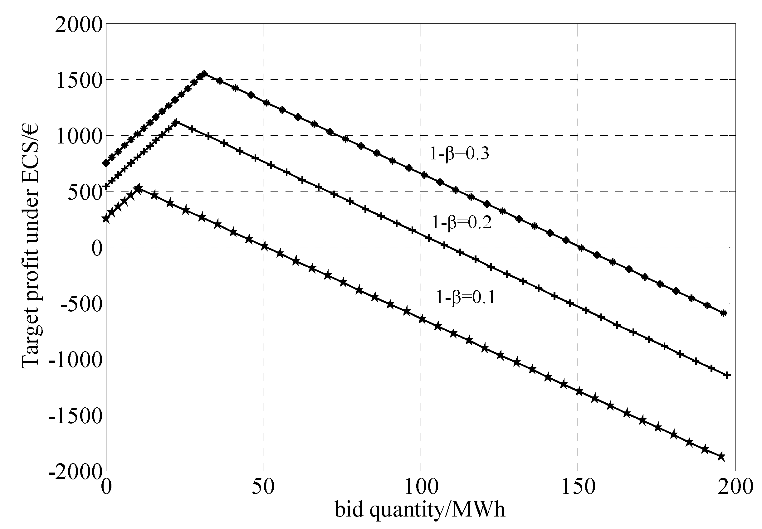


| 1 − β | (€) | (€) | (€) | (€) | F1 in square box (€) | F2 in square box (€) |
|---|---|---|---|---|---|---|
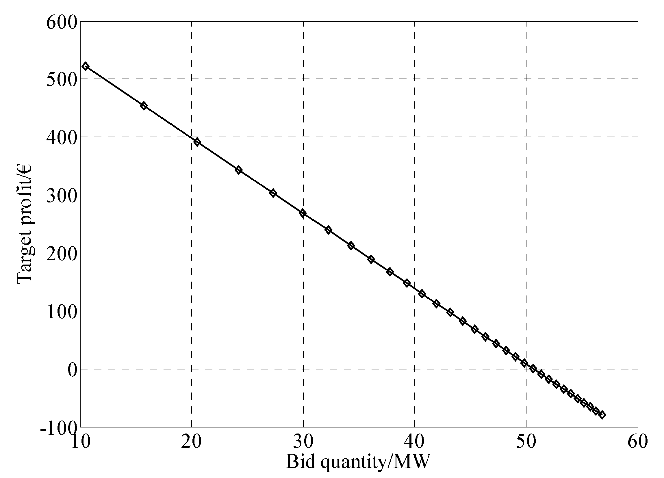
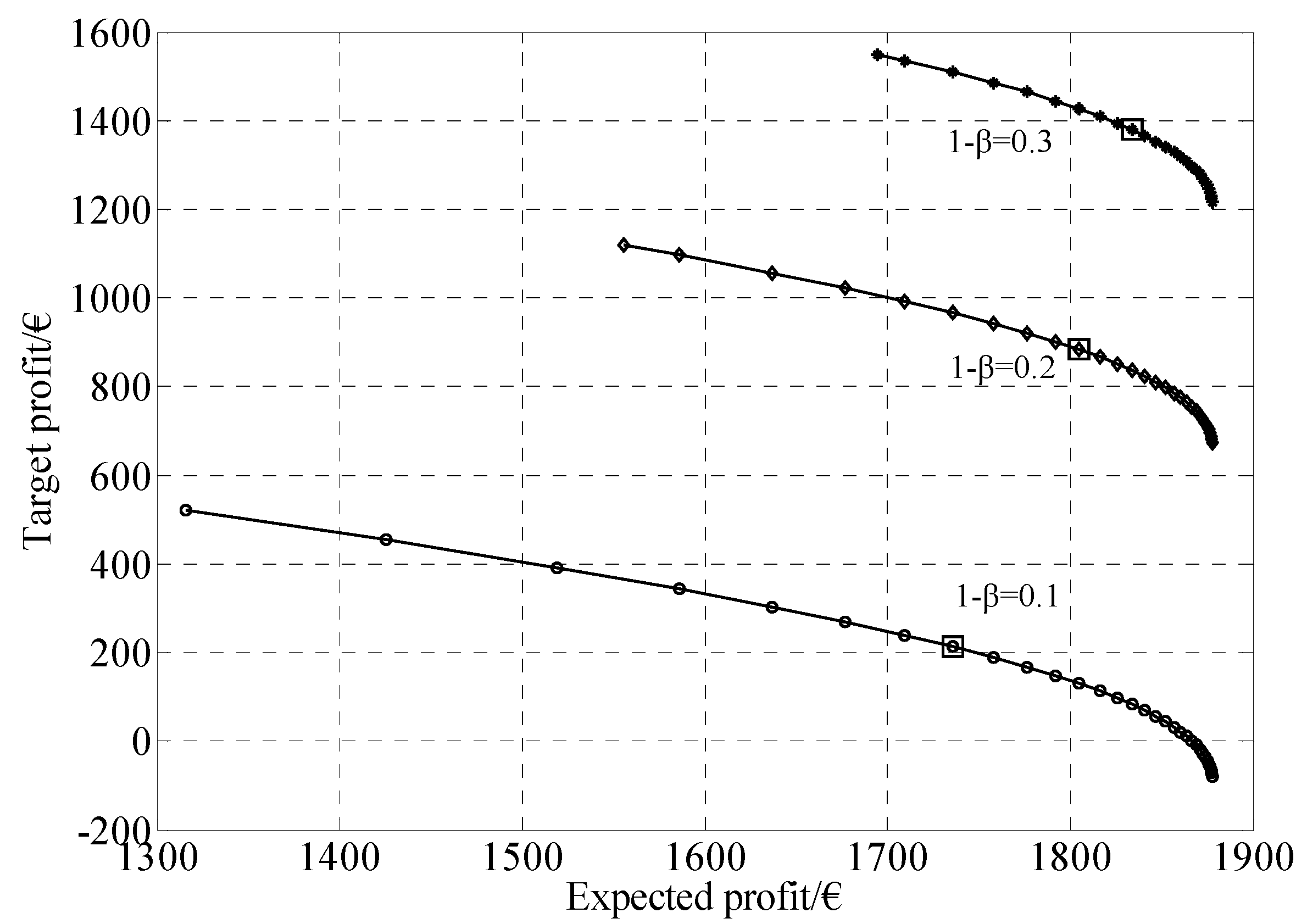
| 0.1 | 1316 | 1877.7 | −79.11 | 521.46 | 1747.4 | 200.72 |
| 0.2 | 1555.9 | 1877.7 | 674.35 | 1119 | 1798.6 | 892.1 |
| 0.3 | 1694.8 | 1877.7 | 1217.7 | 1549.9 | 1839.9 | 1379.5 |


| Standard deviation | EPS | CPS (1 − β = 0.1) | ECPS (1 − β = 0.1) | ||||
|---|---|---|---|---|---|---|---|
| pb | F1 | pb | F2 | pb | F1 | F2 | |
| 4.32 | 47.33 | 2201.5 | 39.96 | 1987 | 43.87 | 2180.9 | 1936.3 |
| 14.18 | 51.49 | 2062.7 | 27.33 | 1358.7 | 0 | 2062.7 | 1974 |
| 24.04 | 55.66 | 1923.9 | 14.69 | 730.46 | 0 | 1923.9 | 1773.6 |
| 33.90 | 59.83 | 1785.1 | 2.055 | 102.19 | 0 | 1785.1 | 1573.1 |
| 43.76 | 63.99 | 1646.3 | 0 | −663.30 | 33.11 | 1483.8 | −1092.8 |

5. Conclusions
Acknowledgments
List of symbols
| R | profit in single period [€], a random variable |
| Pb | quantity bid into day-ahead market in single period [MW] |
| Pt | real power generated by the concerned wind farm [MW] |
| Ic | Imbalance costs in single period [€] |
| Pmax | rated power of the concerned wind farm [MW] |
| λs | day-ahead market price in single period [€/MWh] |
| λsell | price of positive imbalances incurred in single period [€/MWh] |
| λbuy | price of negative imbalances incurred in single period [€/MWh] |
| μt | mean value of wind power forecast in single period t [MW] |
| δt | standard deviation of wind power forecast in single period t [MW] |
| J | target profit in single period[€] |
| β | confidence level, β [0,1] |
| f(Pt) | probability density function of random variable Pt |
| h(R) | probability density function of random variable R |
| H(R) | cumulative distribution function of random variable R |
| Pr{A} | probability of event A |
| F1(Pb) | expected profit function in single period [€] |
| F2(Pb) | target profit function in single period [€] |
| G(Pb) | weighted sum of F1(Pb) and F2(Pb) |
| α | weight assigned to G(Pb) |
maximal value of single objective, i = 1,2 | |
minimal value of single objective, i = 1,2 | |
| uFi | membership function of Fi |
| uD | normalized membership function |
| M | number of nondominated solutions |
| Nobj | number of objectives, in this article, Nobj = 2 |
References
- Holttinen, H. Optimal electricity market for wind power. Energy Policy 2005, 33, 2052–2063. [Google Scholar] [CrossRef]
- Sánchez, I. Short-term prediction of wind energy production. Int. J. Forecast. 2006, 22, 43–56. [Google Scholar] [CrossRef]
- Gao, Y.L.; Pan, J.Y.; Ji, G.L.; Gao, F. A time-series modeling method based on the boosting gradient-descent theory. Sci. China Technol. Sci. 2011, 54, 1325–1337. [Google Scholar] [CrossRef]
- Usaola, J.; Angarita, J. Bidding Wind Energy under Uncertainty. In Proceedings of the International Conference on Clean Electrical Power, Capri, Italy, 21–23 May 2007; pp. 754–759.
- Bathurst, G.N.; Weatherill, J.; Strbac, G. Trading wind generation in short term energy markets. IEEE Trans. Power Syst. 2002, 17, 782–789. [Google Scholar] [CrossRef]
- Fabbri, A.; Roman, T.G.S.; Abbad, J.R.; Quezada, V.H.M. Assessment of the cost associated with wind generation prediction errors in a liberalized electricity market. IEEE Trans. Power Syst. 2005, 20, 1440–1446. [Google Scholar] [CrossRef]
- Pinson, P.; Chevallier, C.; kariniotakis, G.N. Trading wind generation form short-term probabilistic forecasts of wind power. IEEE Trans. Power Syst. 2007, 22, 1148–1156. [Google Scholar] [CrossRef]
- Matevosyan, J.; soder, L. Minimization of imbalance cost trading wind power on the short-term power market. IEEE Trans. Power Syst. 2006, 21, 1396–1404. [Google Scholar] [CrossRef]
- Pousinbo, H.M.I.; Mendes, V.M.F.; Catalao, J.P.S. A stochastic programming approach for the development of offering strategies for a wind power producer. Electr. Power Syst. Res. 2012, 89, 45–53. [Google Scholar] [CrossRef]
- Galloway, S.; Bell, G.; McDonald, J.; Siewierski, T. Managing the risk of trading wind energy in a competitive market. IEE Proc.-Gener. Transm. Distrib. 2006, 153, 106–114. [Google Scholar] [CrossRef]
- Xue, Y.S.; Venkatesh, B.; Chang, L.C. Bidding Wind Power in Short-Term Electricity Market Based on Multiple-Objective Fuzzy Optimization. In Proceedings of 21st Canadian Conference on Electrical and Computer Engineering, Niagara Falls, Canada, 4–7 May 2008; pp. 1135–1138.
- Dukpa, A.; Duggal, I.; Venkatesh, B.; Chang, L. Optimal participation and risk mitigation of wind generators in an electricity market. IET Renew. Power Gener. 2010, 4, 165–175. [Google Scholar] [CrossRef]
- Botterud, A.; Wang, J.; Bessa, R.J.; Keko, H.; Miranda, V. Risk Management and Optimal Bidding for a Wind Power Producer. In Proceedings of IEEE Power and Energy Society General Meeting, Minneapolis, MN, USA, 25–29 July 2010; pp. 1–8.
- Botterud, A.; Zhou, Z.; Wang, J.H.; Bessa, R.J.; Keko, H.; Sumaili, J.; Miranda, V. Wind power trading under uncertainty in LMP markets. IEEE Trans. Power Syst. 2012, 27, 894–903. [Google Scholar] [CrossRef]
- Morales, J.M.; Conejo, A.J.; Pérez-Ruiz, J. Short-term trading for a wind power producer. IEEE Trans. Power Syst. 2010, 25, 554–564. [Google Scholar] [CrossRef]
- Rahimiyan, M.; Morales, J.M.; Conejo, A.J. Evaluating alternative offering strategies for wind producers in a pool. Appl. Energy 2011, 88, 4918–4926. [Google Scholar] [CrossRef]
- Moreno, M.A.; Bueno, M.; Usaola, J. Evaluating risk-constrained bidding strategies in adjustment spot markets for wind power producers. Int. J. Electr. Power Energy Syst. 2012, 43, 703–711. [Google Scholar] [CrossRef]
- Catalao, J.P.S.; Pousinho, H.M.I.; Mendes, V.M.F. Optimal offering strategies for wind power producers considering uncertainty and risk. IEEE Syst. J. 2012, 6, 270–277. [Google Scholar] [CrossRef]
- Dent, C.J.; Bialek, J.W.; Hobbs, B.F. Opportunity cost bidding by wind generators in forward markets: analytical results. IEEE Trans. Power Syst. 2011, 26, 1600–1608. [Google Scholar] [CrossRef] [Green Version]
- Wang, Q.F.; Guan, Y.P.; Wang, J.H. A chance-constrained two-stage stochastic program for unit commitment with uncertain wind power output. IEEE Trans. Power Syst. 2012, 27, 206–215. [Google Scholar] [CrossRef]
- Munoz, J.I.; Contreras, J.; Caamano, J.; Correia, P.F. A decision-making tool for project investments based on real options: the case of wind power generation. Ann. Oper. Res. 2011, 186, 465–490. [Google Scholar] [CrossRef]
- Doherty, R.; O’Malley, M. A new approach to quantify reserve demand in systems with significant installed wind capacity. IEEE Trans. Power Syst. 2005, 20, 587–595. [Google Scholar] [CrossRef]
- Al-Awami, A.T.; El-Sharkawi, M.A. Coordinated trading of wind and thermal energy. IEEE Trans. Sustain. Energy 2011, 2, 277–287. [Google Scholar] [CrossRef]
- Castronuovo, E.D.; Pecas-Lopes, J.A. On the optimization of the daily operation of a wind-hydro power plant. IEEE Trans. Power Syst. 2004, 19, 1599–1606. [Google Scholar] [CrossRef]
- Abido, M.A. Environmental/economic power dispatch using multi-objective evolutionary algorithms. IEEE Trans. Power Syst. 2003, 18, 1529–1537. [Google Scholar] [CrossRef]
- EPEX SPOT SE: Auction. Available online: https://www.epexspot.com/en/market-data/auction/auction-table/2012-03-08/FR (accessed on 26 March 2012).
© 2012 by the authors; licensee MDPI, Basel, Switzerland. This article is an open access article distributed under the terms and conditions of the Creative Commons Attribution license (http://creativecommons.org/licenses/by/3.0/).
Share and Cite
Zhang, H.; Gao, F.; Wu, J.; Liu, K.; Liu, X. Optimal Bidding Strategies for Wind Power Producers in the Day-ahead Electricity Market. Energies 2012, 5, 4804-4823. https://doi.org/10.3390/en5114804
Zhang H, Gao F, Wu J, Liu K, Liu X. Optimal Bidding Strategies for Wind Power Producers in the Day-ahead Electricity Market. Energies. 2012; 5(11):4804-4823. https://doi.org/10.3390/en5114804
Chicago/Turabian StyleZhang, Haifeng, Feng Gao, Jiang Wu, Kun Liu, and Xiaolin Liu. 2012. "Optimal Bidding Strategies for Wind Power Producers in the Day-ahead Electricity Market" Energies 5, no. 11: 4804-4823. https://doi.org/10.3390/en5114804