Impact of PHEVs Penetration on Ontario’s Electricity Grid and Environmental Considerations

Abstract

Plug-in hybrid electric vehicles (PHEVs) have a large potential to reduce greenhouse gases emissions and increase fuel economy and fuel flexibility. PHEVs are propelled by the energy from both gasoline and electric power sources. Penetration of PHEVs into the automobile market affects the electrical grid through an increase in electricity demand. This paper studies effects of the wide spread adoption of PHEVs on peak and base load demands in Ontario, Canada. Long-term forecasting models of peak and base load demands and the number of light-duty vehicles sold were developed. To create proper forecasting models, both linear regression (LR) and non-linear regression (NLR) techniques were employed, considering different ranges in the demographic, climate and economic variables. The results from the LR and NLR models were compared and the most accurate one was selected. Furthermore, forecasting the effects of PHEVs penetration is done through consideration of various scenarios of penetration levels, such as mild, normal and aggressive ones. Finally, the additional electricity demand on the Ontario electricity grid from charging PHEVs is incorporated for electricity production planning purposes.

1. Introduction

The transportation sector is one of the main energy consumption sectors. Technologies for vehicles have been developed over many decades to improve performance, reduce energy consumption, and reduce pollution released into the environment [1]. Plug-in hybrid electric vehicles (PHEVs) combine the combustion engine of conventional vehicles and the electric motor of electric vehicles. PHEVs have greater fuel efficiency because they consume less fuel than in conventional vehicles in which gasoline is the only energy source. PHEVs battery can be recharged by connecting into the electrical grid. This makes PHEVs “fuel flexible vehicles” because they can use both gasoline and electricity for propulsion [2]. One of the important characteristics of PHEVs is their environmental impact. Although PHEVs can reduce the emissions from tailpipe to the environment, the emission shifts to the power plant where electricity may be produced from fossil fuel power plants [3]. However, if electricity is produced from nuclear, solar, hydro or wind power plants, emissions from the power plant become almost zero. Ontario Power Generation (OPG), an Ontario-based electricity generation company, attempts to minimize the environmental impact from their power plants in many ways. OPG plans to phase out their coal plants by the end of 2014 [4]. Nowadays, approximately 78 percent of OPG’s electricity production is generated from hydroelectric and nuclear generating stations [5]. These stations produce a lot less emissions than from fossil fuel power plants that contribute to global warming.

Several automobile manufacturers have produced PHEVs commercially since the end of 2010 [6]. When PHEVs penetrate the automobile market, gasoline consumption will decrease, but electricity demand will subsequently increase [7]. The next challenge of PHEVs is to know whether the electricity grid is capable of supplying the increased electricity demand from charging PHEVs. Electricity needs long-term load forecasts since it takes many years to plan and increase capacity of existing power plants and to build new power plants. For this reason, this study focuses on long-term load forecasting to estimate whether the supplied electricity can meet additional demands from charging PHEVs. Mohamed and Bodger [8] developed a model for long-term forecast of the annual electricity consumption in New Zealand by using the multiple linear regression (LR) method. Explanatory variables that influence the forecast model were gross domestic product (GDP), average price of electricity, and population. Pao [9] developed LR and non-linear regression (NLR) in terms of artificial neural network models to forecast the monthly electricity consumption in Taiwan. National income, population, GDP and consumer price product were proposed as explanatory variables. Chui et al. [10] focused on the long-term forecasting of electricity demand for Ontario, Canada, such as the annual energy, peak load and base load demand using autoregressive, simple LR models (LRMs) and multiple LRMs. The list of potential explanatory variables included GDP, GDP per capita, number of people employed, population, dwelling counts, Heating Degree Days (HDD), and Cooling Degree Days (CDD). Hadley [11] studied the impact of PHEVs on the electricity grid of the VACAR sub-region (North and South Carolina and much of Virginia) in 2018. He assumed that the market share for PHEVs in 2018 is 25%. Yu [12] investigated the impact of PHEVs charge profiles on generation expansion by assuming high PHEVs penetration of 53% in 2030. Hajimiragha et al. [13] performed a feasibility analysis of optimal Ontario’s electricity grid utilization for charging PHEVs during off-peak period. They studied two different transitions of PHEVs penetration. First transition presumes a sluggish penetration of PHEV, especially from 2009 to 2015, with a quicker slope after 2015. The second transition assumes a quick penetration of PHEV between 2009 and 2015 and slow one after that.

In forecasting electricity consumption, most of the literature employed weather, demographic and economic variables as explanatory variables. Moreover, results from NLR models (NLRMs) yield better forecast performance than those from LRMs. Therefore, this study focuses on the impact of those explanatory variables on the model and also compares the mean error between LRMs and NLRMs in order to choose the best model to represent peak and base load demands and the number of light-duty vehicles sold. For PHEV charging, both peak and off-peak charging are considered. Charging of PHEVs during the off-peak period is the best case, in the sense that it has a lower impact on the grid than charging during the peak period. However, not all people would charge their PHEVs during the off-peak period and there is a probability associated with charging in the peak-period. Thus, it is necessary to study the effect of charging in both periods.

2. Issues and Assumptions

It is assumed that PHEVs are commercially produced starting January, 2012. Besides, only new light-duty vehicles are considered as potentially new PHEVs since they have more potential to be PHEVs. Batteries capacity is another issue, especially for charging patterns. Deeper battery charging and discharging cycles than conventional hybrids are required for PHEVs. Since battery life is influenced by the number of full cycles; PHEVs battery life may be smaller than in traditional HEVs which do not deplete their batteries as much as PHEVs [14]. In addition, design issues and trade-offs against battery life, capacity, heat dissipation, weight, costs, and safety are batteries limitations. In this work 80% safety factor and 82% of charger efficiency are assumed [15]. To calculate the demand from charging, identification of types of PHEVs that will penetrate the transportation sector is essential. Based on the average commuting distance in Ontario, 12.9 km, PHEV-20 is assumed to be the main PHEV that will penetrate the light-duty vehicles sector. Another assumption is that no PHEVs are retired during the period under study, 2012–2030.

3. Methodology

The methodology used in this study consists of five steps. Details of each step are described in the following.

3.1. STEP1: Study and Data Collection

Different forecast techniques and model selection criteria are studied to choose a suitable method. Both LR and NLR techniques are employed to create proper forecast models. Dependent variables are peak and base load demands (PEAK and BASE) and light-duty vehicles sold (VEH). Peak load demand is the maximum demand in each day normally occurring between 9 a.m. and 9 p.m. For base load demand, it is defined as the minimum amount of power that power plants must make available to customers. It can be calculated by averaging daily demands in a weekday. Explanatory variables that may impact the PEAK and BASE models are broadly divided into three groups: (I) weather variables such as temperature (T), relative humidity (RH) and wind speed (WS), (II) demographic variable such as population size (POP), income (INC), number of employments (EMP), and (III) economic variable which is gross domestic product (GDP).To forecast VEH, the number of new graduated students (EDU) is also an important factor. People who get degrees at the undergraduate and graduate level tend to buy new cars more than others [16]. Therefore, the number of graduated students is one of the explanatory variables to forecast the number of light-duty vehicles sold.

Historical data of dependent and explanatory variables are collected to fulfill the required data for developing the models. Before achieving historical data of peak and base load demand, outlier determination is an important step in order to avoid poor forecasting results. In this study, Statistics Package for Social Science (SPSS) version 20.0 [17] was used to develop the forecast models. SPSS also has a feature to identify outliers among inputs by using boxplot. All outliers are omitted from the data and replaced by the values at the closest boundary. An important possible issue with explanatory variables is multicollinearity problems. Multicollinearity occurs when two or more explanatory variables are highly correlated. As a result, regression procedures may not be able to distinguish between the separate contributions of these variables to the dependent variable, and the estimation of unknown parameters may be unreliable. Ordinary multicollinearity is the situation in which there is a close, but not perfect, linear relationship between some of the explanatory variables in the sample data. Multicollinearity is usually considered to be a data or sample problem. The principle of parsimony (using the simpler model when greater complexity does not provide significant benefits) suggests that when two or more variables are highly correlated, one of them should be omitted from the model. Matrix scatter in SPSS is used for detecting multicollinearity. The scatter that presents linear relationship between two explanatory variables indicates multicollinearity problem.

3.2. STEP2: Model Development and Selection

In this step, models for forecasted peak and base load demands and light-duty vehicles sold were developed using LRMs and NLRMs. Historical data of peak and base load demands were monthly data from 1994 to 2010 [18]. Those data and hourly load demand in 2010 were obtained from the Independent Electricity System Operator (IESO) [19]. To simplify the forecasting, four months representing each season were used as input in the model development. Hence, eight models were developed to represent peak and base load demands for the four selected months. Four of them are used for forecasting peak load demand and the rest are used for forecasting base load demand.

For historical light-duty vehicles sold, information was provided by season. Therefore, one model was formulated to represent light-duty vehicles sold in all seasons, with only some model parameters being changed to distinguish the four seasons.

3.2.1. Linear Regression with SPSS

To formulate a LRM in SPSS, dependent and explanatory variables need to be defined. Details of these variables were discussed in the first step. A list of variables used as input of SPSS is summarized in Table 1, where PEAK, BASE, VEH represent peak and base load demand and light duty vehicles sold. T, RH, WS, POP, INC, EMP, EDU, GDP are temperature, relative humidity, wind speed, population size, income, number of people employed, number of new graduated students and gross domestic product respectively. But some of these explanatory variables are highly correlated to each other. For example, when there are more new graduate students, there will be a higher number of people employed. Also wind speed and relative humidity are highly correlated for some temperatures (in particular for the extreme high and low ones).

Table 1. Input variables for linear regression.

Dependent variables	Explanatory variables
PEAK, ln(PEAK)	T, RH, WS, POP, INC, EMP, GDP, ln(T), ln(RH), ln(WS), ln(POP), ln(INC), ln(EMP), ln(GDP)
BASE, ln(BASE)
VEH, ln(VEH)	POP, INC, EMP, EDU, GDP, ln(POP), ln(INC), ln(EMP), ln(EDU), ln(GDP)

Table 1. Input variables for linear regression.

Dependent variables	Explanatory variables
PEAK, ln(PEAK)	T, RH, WS, POP, INC, EMP, GDP, ln(T), ln(RH), ln(WS), ln(POP), ln(INC), ln(EMP), ln(GDP)
BASE, ln(BASE)
VEH, ln(VEH)	POP, INC, EMP, EDU, GDP, ln(POP), ln(INC), ln(EMP), ln(EDU), ln(GDP)

To determine which combination of explanatory variables provides the best fit to the data, SPSS has an automated process for variable selection called “stepwise regression” in which the regression equation is automatically estimated several times.

3.2.2. Non-Linear Regression with SPSS

NLR in SPSS does not have a tool to choose the best combination of explanatory variables unlike LR. Therefore, selecting a set of explanatory variables should be done manually. To reduce complexity, only multiple NLRMs were considered which means only two explanatory variables were used as input of the models. In addition, pairing of explanatory variables which are highly correlated must be omitted to prevent the multicollinearity problem. Logarithm terms of both dependent and explanatory variables were not included. Possible combinations of explanatory variables are illustrated in Table 2.

Table 2. Possible explanatory variables combination for NLR.

Dependent variables	Combination of explanatory variables
PEAK	T vs. RH	RH vs. WS	WS vs. POP
BASE	T vs. WS	RH vs. POP	WS vs. INC
	T vs. POP	RH vs. INC	WS vs. EMP
	T vs. INC	RH vs. EMP	WS vs. GDP
	T vs. EMP	RH vs. GDP
	T vs. GDP

Table 2. Possible explanatory variables combination for NLR.

Dependent variables	Combination of explanatory variables
PEAK	T vs. RH	RH vs. WS	WS vs. POP
BASE	T vs. WS	RH vs. POP	WS vs. INC
	T vs. POP	RH vs. INC	WS vs. EMP
	T vs. INC	RH vs. EMP	WS vs. GDP
	T vs. EMP	RH vs. GDP
	T vs. GDP

After finding all possible LRMs and NLRMs, the next step is model selection. Mean Absolute Error, MAE, Mean Squared Error, MSE, and Mean Absolute Percentage Error, MAPE, were employed as a criterion for selecting the best model. The model that has the lowest MAE, MSE and MAPE were chosen to represent the historical data and also forecast future data. The equation of MAE, MSE and MAPE can be written as follows:

$$MAE=\frac{{{\displaystyle \sum }}_{t=1}^n\left|e_t\right|}{n}=\frac{{{\displaystyle \sum }}_{t=1}^n\left|y_t-{\widehat{y}}_t\right|}{n}$$

(1)

$$MSE=\frac{{{\displaystyle \sum }}_{t=1}^n{\left(e_t\right)}^2}{n}=\frac{{{\displaystyle \sum }}_{t=1}^n{\left(y_t-{\widehat{y}}_t\right)}^2}{n}$$

(2)

$$MAE=\frac{{{\displaystyle \sum }}_{t=1}^n\left(100*\left|e_t\right|/y_t\right)}{n}=\frac{{{\displaystyle \sum }}_{t=1}^n\left(100*\left|y_t-{\widehat{y}}_t\right|/y_t\right)}{n}$$

(3)

where e_t is the error term, n is the total number of observations and t is time index. y_t and ${\widehat{y}}_t$ are the observed and estimated values, respectively.

3.3. STEP 3: Projection of Forecast Variables

The best models for forecasting peak and base load demands and light-duty vehicles sold were used for projecting the future value of those dependent variables from 2012 to 2030. Future values of all explanatory variables shown in the selected models were substituted into those models in order to predict values of the dependent variables.

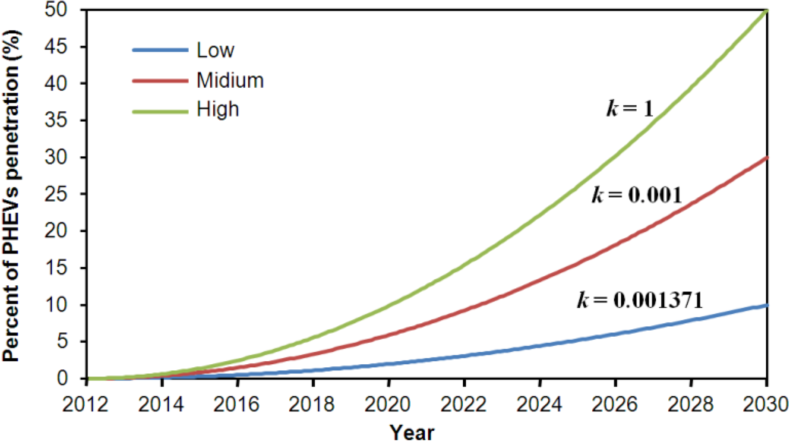
3.4. STEP 4: Study of PHEVs Penetration and Charging Pattern

Since PHEVs were not commercially produced before January 2012, this study assumes that there is no PHEV in January, 2012. Three transition models of PHEVs penetration in the light-duty vehicles sold, named low, medium and high, are shown in Figure 1 assuming 10%, 30% and 50% of PHEVs penetration by December, 2030, respectively. These equations are used because of being more straightforward than the exponential equations during mentioned time period. For all models a constant penetration rate for any given scenario is assumed:

$$PHEVs=k\times t^2$$

(4)

where PHEVs is the number of PHEVs, k is the constant rate and t is time. In this study, only new light-duty vehicles are considered. Before studying charging patterns, it is necessary to identify which type of PHEVs will penetrate into the transportation sector. To choose appropriate types of PHEVs that match people’s lifestyle in Ontario, commuting distance must be considered.

Figure 1. Percent of PHEV penetration in Ontario.

Figure 1. Percent of PHEV penetration in Ontario.

Table 3 compares commuting distances in Canada and Ontario [20]. The average commuting distance in Ontario is 12.9 km (= 8 miles). This implies that PHEV-20, which can travel twenty miles without using its combustion engine, is appropriate for a majority of people in Ontario. Therefore, this study assumes that only PHEV-20 penetrates into the light-duty vehicles sold. Another assumption is that no PHEVs are retired during the period under study. Since most household outlets already contain 120 V/15 A outlets, it is assumed that all PHEV-20 will be recharged through this circuit every day. Charger requirements of PHEV-20 with 120 V/15 A outlets are summarized in Table 4.

Table 3. Average commuting distance in Canada and Ontario [12].

Commuting distance (km)	Commuters (people)
	Canada	Ontario
Less than 5 km	4,741,630	1,672,260
5–9.9 km	2,962,810	1,101,410
10–14.9 km	1,738,750	672,685
15–19.9 km	1,095,465	475,410
20–24.9 km	693,645	318,960
25–29.9 km	461,250	213,460
30 km or more	1,376,340	640,470
Average commuting distance (km)	11.9	12.9

Table 3. Average commuting distance in Canada and Ontario [12].

Commuting distance (km)	Commuters (people)
	Canada	Ontario
Less than 5 km	4,741,630	1,672,260
5–9.9 km	2,962,810	1,101,410
10–14.9 km	1,738,750	672,685
15–19.9 km	1,095,465	475,410
20–24.9 km	693,645	318,960
25–29.9 km	461,250	213,460
30 km or more	1,376,340	640,470
Average commuting distance (km)	11.9	12.9

Table 4. Charger requirements for PHEV-20 under 120 V/15 A outlets [13,14].

Vehicle type	Rated pack size (kWh)		Charging size a	Charger rate b
	20 miles	8 miles	(kW)	(kW)
Compact Car	4.10	1.64	1.44	1.18
Mid-Sized Sedan	4.70	1.88	1.44	1.18
Mid-Sized SUV	6.30	2.52	1.44	1.18
Full-Sized SUV	7.40	2.96	1.44	1.18
Average	5.63	2.25	1.44	1.18

Note: ^a An 80% required safety factor for continuous charging is used; ^b Charger efficiency is assumed to be 82%.

Table 4. Charger requirements for PHEV-20 under 120 V/15 A outlets [13,14].

Vehicle type	Rated pack size (kWh)		Charging size a	Charger rate b
	20 miles	8 miles	(kW)	(kW)
Compact Car	4.10	1.64	1.44	1.18
Mid-Sized Sedan	4.70	1.88	1.44	1.18
Mid-Sized SUV	6.30	2.52	1.44	1.18
Full-Sized SUV	7.40	2.96	1.44	1.18
Average	5.63	2.25	1.44	1.18

Note: ^a An 80% required safety factor for continuous charging is used; ^b Charger efficiency is assumed to be 82%.

New peak and base load demands represent PHEVs charging in peak and off-peak period, respectively. They can be calculated by adding the amount of PHEVs charging in each period with peak and base load demands obtained from regression models. Equations for calculation new peak and base load demands are shown below:

$$Pea{k}_{n,i}=Pea{k}_{r,i}+\frac{BS\times PHEV{s}_p}{5hrs}$$

(5)

$$Bas{e}_{n,i}=Bas{e}_{r,i}+\frac{BS\times PHEV{s}_{op}}{5hrs}$$

(6)

where Peak_n,i and Base_n,i are new peak and base load demands after adding the amount of PHEVs charging, respectively. Peak_r,i and Base_r,i are peak and base load demands obtained from regression models, respectively. PHEVs_p and PHEVs_op are number of PHEVs charging in peak and off-peak periods, respectively. BS is the battery size or the rated pack size. Through Equations (5) and (6) the peak and base load demand without considering PHEVs are added to the amount of electricity that is needed for charging all of the PHEVs, which is the battery size divided by number of charging hours.

PHEVs can be recharged in both peak periods and off-peak periods. Details of each scenario are illustrated in Table 5. P100 represents the worst case of charging scheme since all PHEVs are assumed to be recharged during the peak period whereas P0 represents the best case which all PHEVs are recharged during the off-peak period.

Table 5. Details of charging scenarios.

Scenario	Percent of PHEVs
	Peak period	Off-peak period
P100	100	0
P75	75	25
P50	50	50
P25	25	75
P0	0	100

Table 5. Details of charging scenarios.

Scenario	Percent of PHEVs
	Peak period	Off-peak period
P100	100	0
P75	75	25
P50	50	50
P25	25	75
P0	0	100

3.5. STEP 5: Comparisons of Worst Case Scenario with Ontario’s Available Resources and Carbon Dioxide Emission Calculation

In this step, the worst case of penetration level and charging scenario is chosen as the case study. The demand of the worst case is compared to available resources in Ontario to see whether there can be enough supply to the increasing demand from PHEVs charging.

As mentioned previously, PHEVs reduce CO₂ emissions from tailpipes. The penetration of PHEVs into the transportation sector shifts emissions to the power plants. The effect on CO₂ emissions is dependent on the fuel sources of the electricity. If electricity is produced from high polluting sources, the environmental benefits of PHEVs are correspondingly limited. However, regulating CO₂ emissions from power plants instead of vehicle tailpipes is more likely. The total CO₂ emissions are calculated by the following equations:

$$TotalC{O}_2=TotalC{O}_2\left(PowerPlants\right)+TotalC{O}_2\left(Vehicles,nonPHEVs\right)+TotalC{O}_{2}PHEVs$$

(7)

$$TotalC{O}_2\left(PowerPlants\right)={\displaystyle \sum }{M}_P\times C{E}_P$$

(8)

$$TotalC{O}_2\left(Vehicle,nonPHEVs\right)={\displaystyle \sum }A{D}_y\times C{E}_V\times N$$

(9)

where CE_P and CE_V are CO₂ emissions in t/MWh and t/km. P and V represent type of power plants and non PHEVs respectively. AD_y and N represent average community distance per year and number of PHEVs. Because average community distance in Ontario is lower than 20 miles, total CO₂ emission from PHEV-20 is considered zero.

4. Model Development

4.1. Peak Load Demand Models

Using the above selection approach, LRMs for peak load demand forecast in January, May, August and October are chosen to be:

$$\mathrm{January}:\ln \left(PEA{K}_i\right)=9.7+5\times {10}^{-7}GD{P}_i-9.1\times {10}^{-3}{T}_i$$

(10)

$$\mathrm{May}:PEA{K}_i=-36,900+4,1400\text{ ln}(GD{P}_i)$$

(11)

$$\mathrm{August}:PEA{K}_i=79,890+6,4400\text{ ln}\left(GD{P}_i\right)+5,20\text{ ln}(T_i)$$

(12)

$$\mathrm{October}:PEA{K}_i=-42,000+4,5900\text{ ln}(GD{P}_i)$$

(13)

The peak load demand in January and August are a function of temperature and GDP, while the peak load demand in May and October are a function of GDP only. Temperature has much effect on the winter and the summer. In the winter [Equation (10)], the temperature is always below zero; therefore, the lower the temperature is, the higher the peak load demand will be. This is because people need more electricity for space heating. On the other hand, during summer (Equation (12)), electricity consumption increases because more electricity is required for space cooling. GDP is the only explanatory variable which affects the peak load demand in all four months. From Equations (10)–(13), all coefficients of GDP are positive; hence, greater number in GDP results in higher peak load demand. The best NLRMs of peak load demand in four selected months are shown below:

$$\mathrm{January}:PEA{K}_i=46,835-24,930\left(\text{exp}(8\times {10}^{-3}{T}_{\mathrm{i}}\right)+\text{exp}(-6.2\times {10}^{-6}GD{P}_i))$$

(14)

$$\mathrm{May}:PEA{K}_i=17,900-73,141\text{ exp}(-{10}^{-5}GD{P}_i)$$

(15)

$$\mathrm{August}:PEA{K}_i=23,000-42,600\left(\text{exp}(-0.2T_{\mathrm{i}}\right)+\text{exp}(-7\times {10}^{-6}GD{P}_i))$$

(16)

$$\mathrm{October}:PEA{K}_i=19,900-18,570\text{ exp}(-4.8\times {10}^{-6}GD{P}_i)$$

(17)

The same trends are found as with LRMs. Temperature affects base load demands in January and August (the seasons corresponding to the highest peaks), while GDP affects base load demand in all four months. All coefficients of NLRMs follow the law of diminishing returns. It means that the results of the models first increase quickly when increasing temperature and GDP and then increase more slowly. For Equation (14), the coefficient of temperature is positive; however, when multiplying with temperature in the winter which is always negative, this term will be negative which follows the law of diminishing returns. All temperatures are given in °C. Note that although the January and August peaks depends on temperatures, those temperatures are assumed constant from one year to the other year and thus the changes in peak demand over the years are due solely to changes in GDP.

4.2. Base Load Demand Models

Using the same selection approach as in the case of peak load demand, the best LRMs and NLRMs of base load demand in January, May, August, and October are shown below:

LRMs:

$$\mathrm{January}:BAS{E}_i=13,500-177T_i+9.4\times {10}^{-3}GD{P}_i$$

(18)

$$\mathrm{May}:BAS{E}_i=-37,000+4,000\text{ ln}(GD{P}_i)$$

(19)

$$\mathrm{August}:BAS{E}_i=73,200+5,650\text{ ln}\left(GD{P}_i\right)+5,650\text{ ln}(T_i)$$

(20)

$$\mathrm{October}:BAS{E}_i=-36,510+4,050\text{ ln}(GD{P}_i)$$

(21)

NLRMs:

$$\mathrm{January}:BAS{E}_i=57,750-22,430\left(\text{exp}(8.3\times {10}^{-3}{T}_i\right)+\text{exp}(-5.5\times {10}^{-7}GD{P}_i))$$

(22)

$$\mathrm{May}:BAS{E}_i=17,260-20,680\text{ exp}(-5.8\times {10}^{-6}GD{P}_i)$$

(23)

$$\mathrm{August}:BAS{E}_i=21,080-42,800\left(\text{exp}(-0.1T_{\mathrm{i}}\right)+\text{exp}(-7.4\times {10}^{-6}GD{P}_i))$$

(24)

$$\mathrm{October}:BAS{E}_i=17,640-16,270\text{ exp}(-5.4\times {10}^{-6}GD{P}_i)$$

(25)

Trends for base load demand forecast are similar to those of peak load demand forecast. Both LRMs and NLRMs of base load demand forecast in January and August depends on the temperature and GDP and those of base load demand forecast in May and October depend only on GDP.

4.3. Light-Duty Vehicles Sold

Best LRMs and NLRMs are shown below:

LRMs:

$$ln(VE{H}_i)=11.1-0.1x_1+0.3x_2+0.1x_3+2.1\times {10}^{-7}GD{P}_i$$

(26)

NLRMs:

$$VE{H}_i=75,840-6,850x_1+24,370x_2+7,780x_3-39,580\text{ exp}(-6.1\times {10}^{-6}GD{P}_i)$$

(27)

where x₁, x₂ and x₃ are integer valued including x₁ = 1 and x₂ = x₃ =0 for winter, x₂ = 1 and x₁ = x₃ = 0 for spring, x₃ = 1 and x₁ = x₂ = 0 for summer and lastly x₁ = x₂ = x₃ = 0 for autumn. Both LRMs and NLRMs of light-duty vehicles sold forecast consist of these integer valued and GDP. From Equations (26) and (27), the number of light-duty vehicles sold increases when increasing GDP because people have more potential to buy new vehicles when the economic growth is positive.

5. Model Selection

Comparisons were made among LRMs and NLRMs. MAE, MSE and MAPE were employed as the criterion to determine which model yields the most accurate results. MAEs, MSEs and MAPEs of all regression models of peak and base load demands and light-duty vehicles sold are compared in Table 6. For peak load demand, NLRMs of all four months yield lower MAEs, MSEs and MAPEs than LRMs. Therefore, NLRMs represented in Equations (14)–(16) were selected to represent peak load demand in January, May, August, and October, respectively. When comparing between LRMs and NLRMs for base load demand, NLRMs in May, August, and October gives smaller MAEs. The opposite result is found in January. The LRM of January yield lower MAE, MSE and MAPE than NLRM. However, the difference between MAE, MSE and MAPE of LRMs and NLRMs is very small (approximately 1.8%). Therefore, the LRM represented by Equation (18) was employed to represent base load demand in January and NLRMs represented by Equations (23)–(25) are used to illustrate base load demand in May, August, and October, respectively. For light-duty vehicles sold, the LRMs gives better results than NLRMs, but there is only a slight difference between the MAEs for both regression models (approximately 0.4%). In this case, the LRM represented by Equation (26) was chosen to represent the number of light-duty vehicles sold due to lower mean absolute error of the model.

In summary, most of NLRMs yield lower MAE than LRMs. This implies that the relationship between forecast variables (peak and base load demands) and explanatory variables (temperature and GDP) are not always linear. In the few cases where LRMs give better results than NLRMs (base load demand in January and light-duty vehicles sold), the differences between MAEs, MSE and MAPE of both regression models are insignificant.

Table 6. Model comparisons.

Forecast variables	MAE		MSE		MAPE		Selected models
	LRM	NLRM	LRM	NLRM	LRM	NLRM
1. Peak load demand
January	307.6	300.3	138,965	124,507	1.45	1.41	NLRM [Equation (14)]
May	323.7	273.0	181,623	142,217	1.90	1.60	NLRM [Equation (15)]
August	443.8	420.7	333,226	301,652	2.22	2.10	NLRM [Equation (16)]
October	415.2	391.4	269,448	247,339	2.34	2.21	NLRM [Equation (17)]
2. Base load demand
January	327.6	333.4	158,877	160,983	1.71	1.74	LRM [Equation (18)]
May	336.4	308.9	208,385	189,852	2.16	1.98	NLRM [Equation (23)]
August	386.2	360.5	292,767	254,423	2.17	2.02	NLRM [Equation (24)]
October	390.3	372.9	211,663	194,546	2.40	2.30	NLRM [Equation (25)]
3. Light-duty vehicles sold	6,699.8	6,848.9	74,529,858	7,697,788	8.62	8.87	LRM [Equation (26)]

Table 6. Model comparisons.

Forecast variables	MAE		MSE		MAPE		Selected models
	LRM	NLRM	LRM	NLRM	LRM	NLRM
1. Peak load demand
January	307.6	300.3	138,965	124,507	1.45	1.41	NLRM [Equation (14)]
May	323.7	273.0	181,623	142,217	1.90	1.60	NLRM [Equation (15)]
August	443.8	420.7	333,226	301,652	2.22	2.10	NLRM [Equation (16)]
October	415.2	391.4	269,448	247,339	2.34	2.21	NLRM [Equation (17)]
2. Base load demand
January	327.6	333.4	158,877	160,983	1.71	1.74	LRM [Equation (18)]
May	336.4	308.9	208,385	189,852	2.16	1.98	NLRM [Equation (23)]
August	386.2	360.5	292,767	254,423	2.17	2.02	NLRM [Equation (24)]
October	390.3	372.9	211,663	194,546	2.40	2.30	NLRM [Equation (25)]
3. Light-duty vehicles sold	6,699.8	6,848.9	74,529,858	7,697,788	8.62	8.87	LRM [Equation (26)]

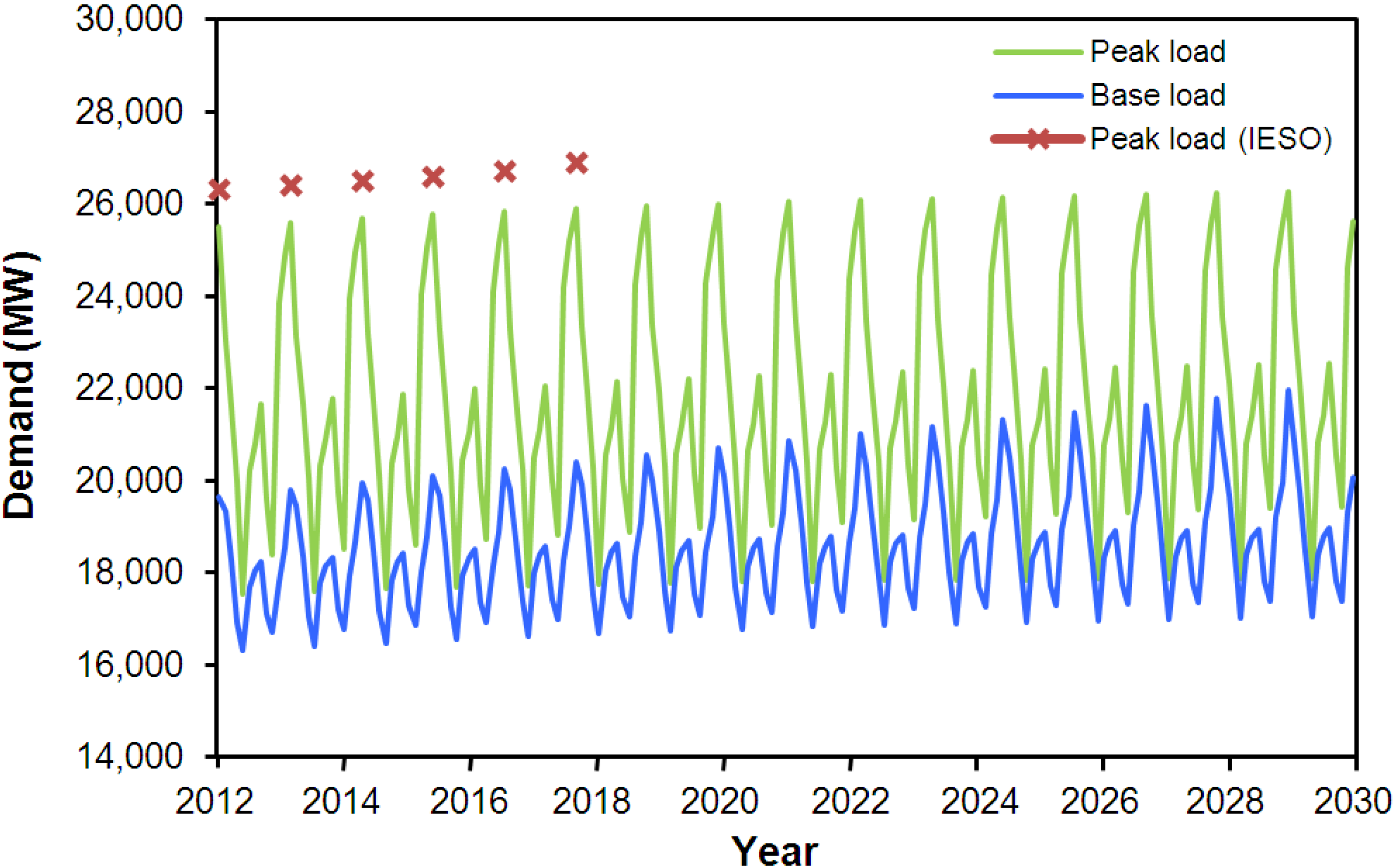
6. Projection of Forecast Variables

From the previous section, the best models for peak and base load demands and light-duty vehicles sold depend upon the temperature and GDP. The projections of peak and base load demands, without PHEVs, and light-duty vehicles sold until 2030 are shown in Figure 2 and Figure 3, respectively.

As shown in Figure 2, the highest peak and base load demands of each year normally occur in January which is approximately 26,000 MW and 21,000 MW, respectively. More electricity is required for space heating in the winter, resulting in greater amount of peak and base load demands in January. IESO also published peak load demand forecast in Ontario from 2012 until 2018. Comparing peak load demand from regression models with IESO forecast, there is an average difference of approximately 3%. Since the forecasting methodology from IESO is not known to us, it is impossible to explain these differences. Nonetheless, these differences are sufficiently small that both models are in reasonable agreement.

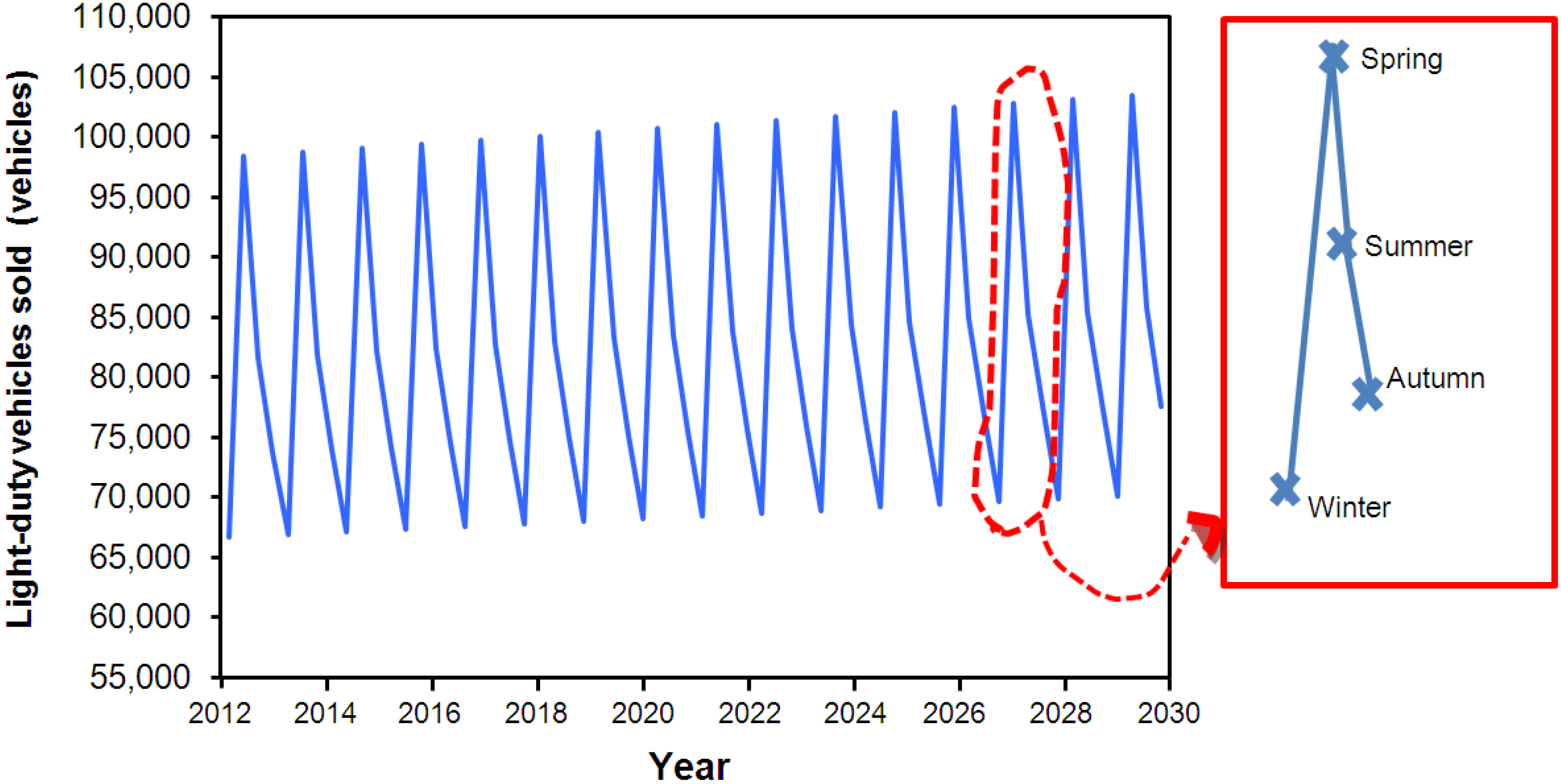
When considering the projection of light-duty vehicles sold (Figure 3), it was found that a majority of light-duty vehicles are sold in the spring. The main reasons are better weather and buying conditions in spring than rest of the year where industries are provided to sell previous year models. The rank of light-duty vehicles sold from high to low is: spring > summer > autumn > winter.

Figure 2. Projection of peak and base load demands.

Figure 2. Projection of peak and base load demands.

Figure 3. Projection of light-duty vehicles sold.

Figure 3. Projection of light-duty vehicles sold.

7. Effects of PHEVs Penetration

In the study of PHEVs penetration, three transitions, low, medium and high, are assumed to represent PHEVs penetration from 2012 to 2030 which was shown in Figure 1. Other assumptions used in PHEVs charging demand calculations are listed below:

• Only PHEV-20 penetrates into Ontario’s transportation sector.
• No PHEVs are retired from 2012 to 2030.
• All PHEVs are recharged through the circuit during the peak period every day (worst case scenario).

Figure 4 represents model’s results of accumulative numbers of PHEVs in the Ontario’s transportation sector in various transitions of PHEVs penetration levels. The total number PHEVs at the end of 2030 for low, medium and high transition will be approximately 178,000, 534,000 and 890,000, respectively.

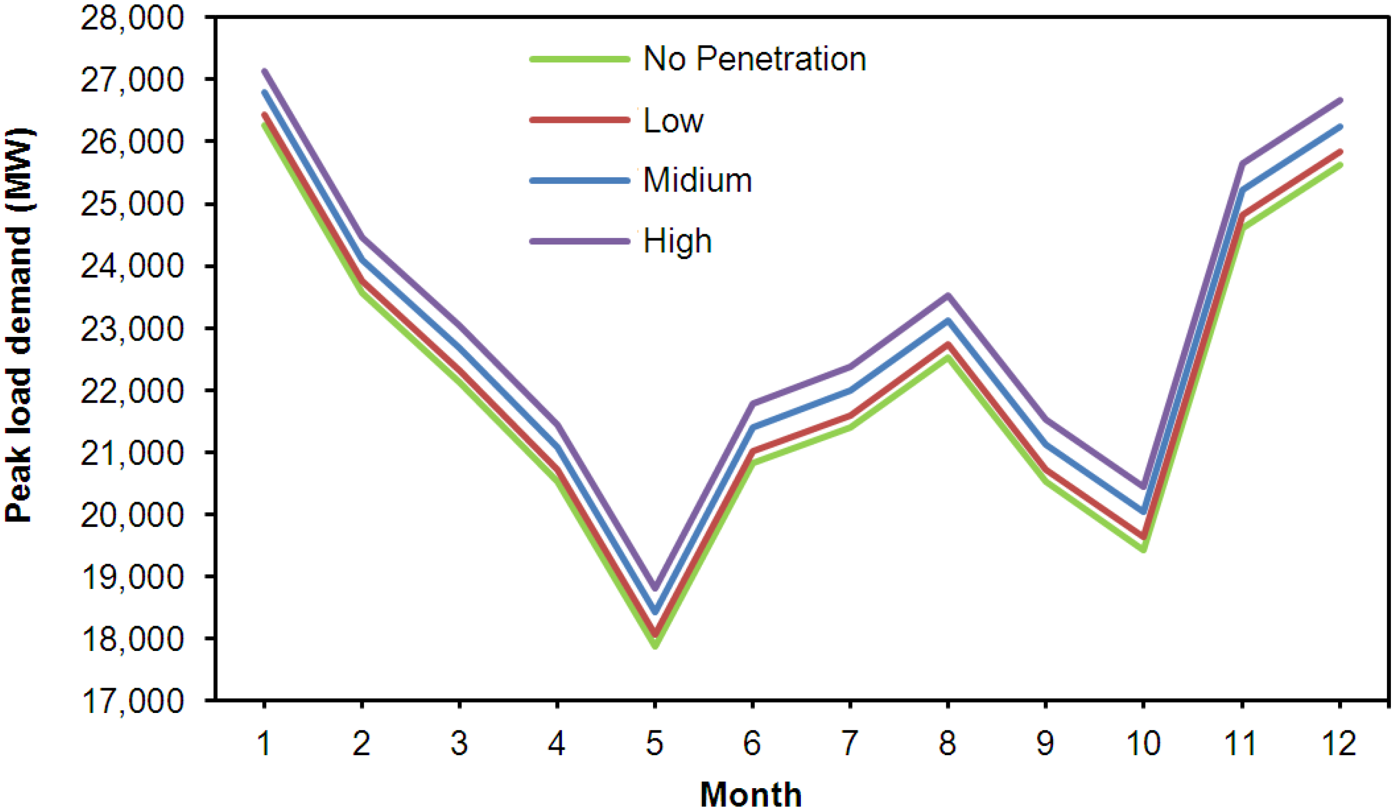
New peak and base load demands after adding PHEVs into the transportation sector can be calculated from Equations (5) and (6), respectively. As illustrated in Figure 5, the peak load demand of PHEVs for high transition is the highest since this transition assumes the greatest amount of PHEVs penetration which is 50% of new vehicles in December, 2030. Additional peak load demands in December, 2030 from PHEVs charging for low, medium and high transitions will be 210.3 MW, 630.8 MW and 1051.3 MW, respectively.

Figure 4. Accumulative numbers of PHEVs in the Ontario’s transportation sector.

Figure 4. Accumulative numbers of PHEVs in the Ontario’s transportation sector.

Figure 5. Comparisons of peak load demand for different transition levels in December 2030.

Figure 5. Comparisons of peak load demand for different transition levels in December 2030.

8. Effects of Charging Patterns

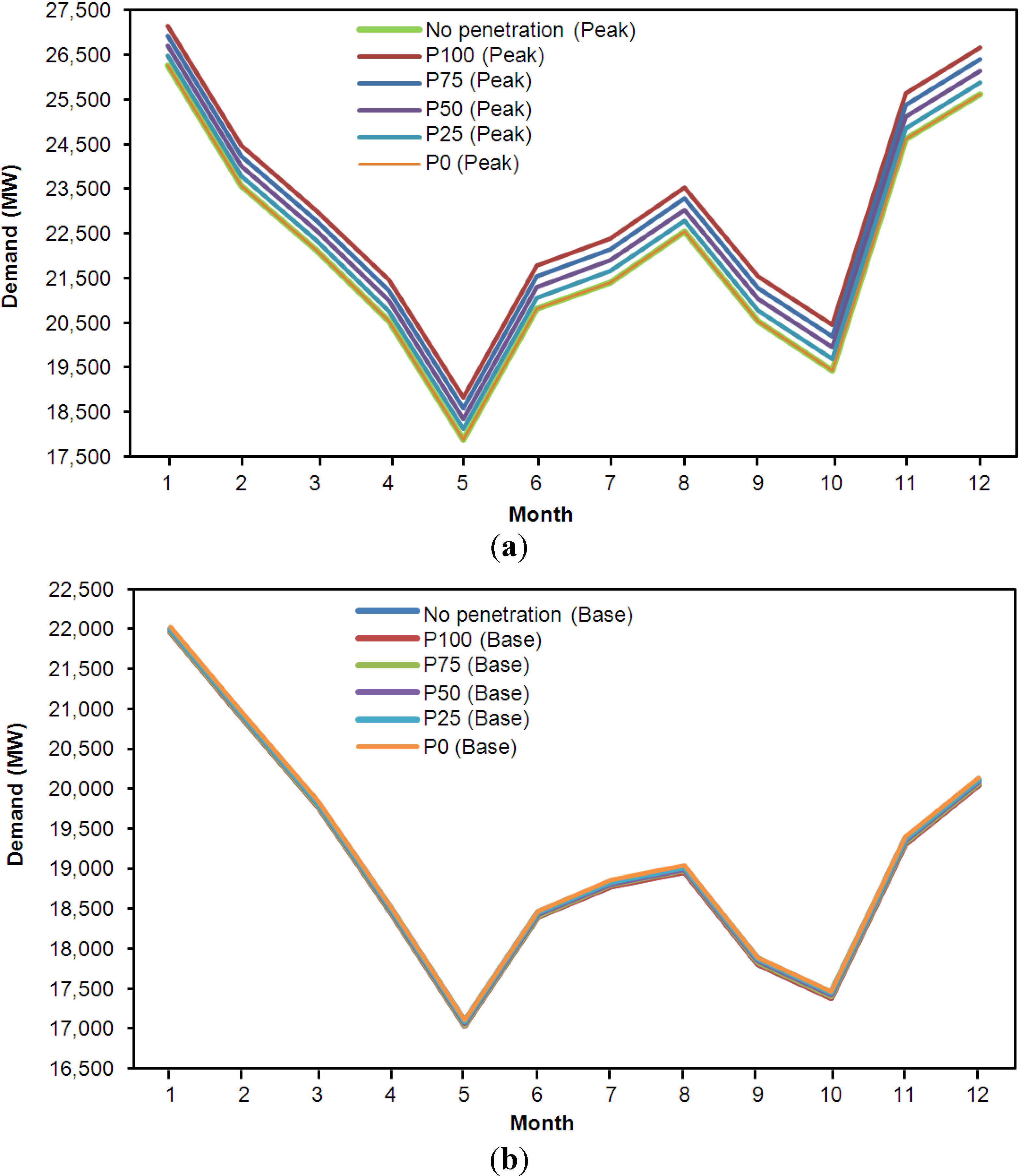
Results of peak and base load demands for different charging scenarios after adding PHEVs into the transportation sector in 2023 (as an example) are shown in Figure 6. As can be seen, the peak load demand from charging pattern in Scenario P100, which represents charging only during the peak period, is the highest among all scenarios. For Scenario P0, its peak load demand is similar to the peak load demand when there is no PHEVs penetration because the number of PHEVs being recharged in the peak period in Scenario P0 is assumed to be zero. Additional peak load demands in December 2023 from PHEVs charging in Scenario P100 to Scenario P0 will be 1,051.3 MW, 788.5 MW, 525.7 MW, 262.8 MW and 0 MW, respectively.

For the base load demand, Scenario P0 in which all PHEVs are recharged during the off-peak period has the highest base load, while base load demand for Scenario P100 in which no PHEVs are recharged during the off-peak period is similar to the base load demand with no PHEVs penetration. From Figure 6, the base load demand in all scenarios is not much different. Additional base load demands in December, 2023 from PHEVs charging in Scenario P100 to Scenario P0 are 0 MW, 20.9 MW, 41.7 MW, 62.6 MW and 83.5 MW, respectively. When comparing additional peak and base load demands in all scenarios, it was found that PHEV charging pattern has more effect on the peak load demand than on the base load demand.

Figure 6. Peak load demands (a) and base load demands (b) in different charging scenarios in 2023.

Figure 6. Peak load demands (a) and base load demands (b) in different charging scenarios in 2023.

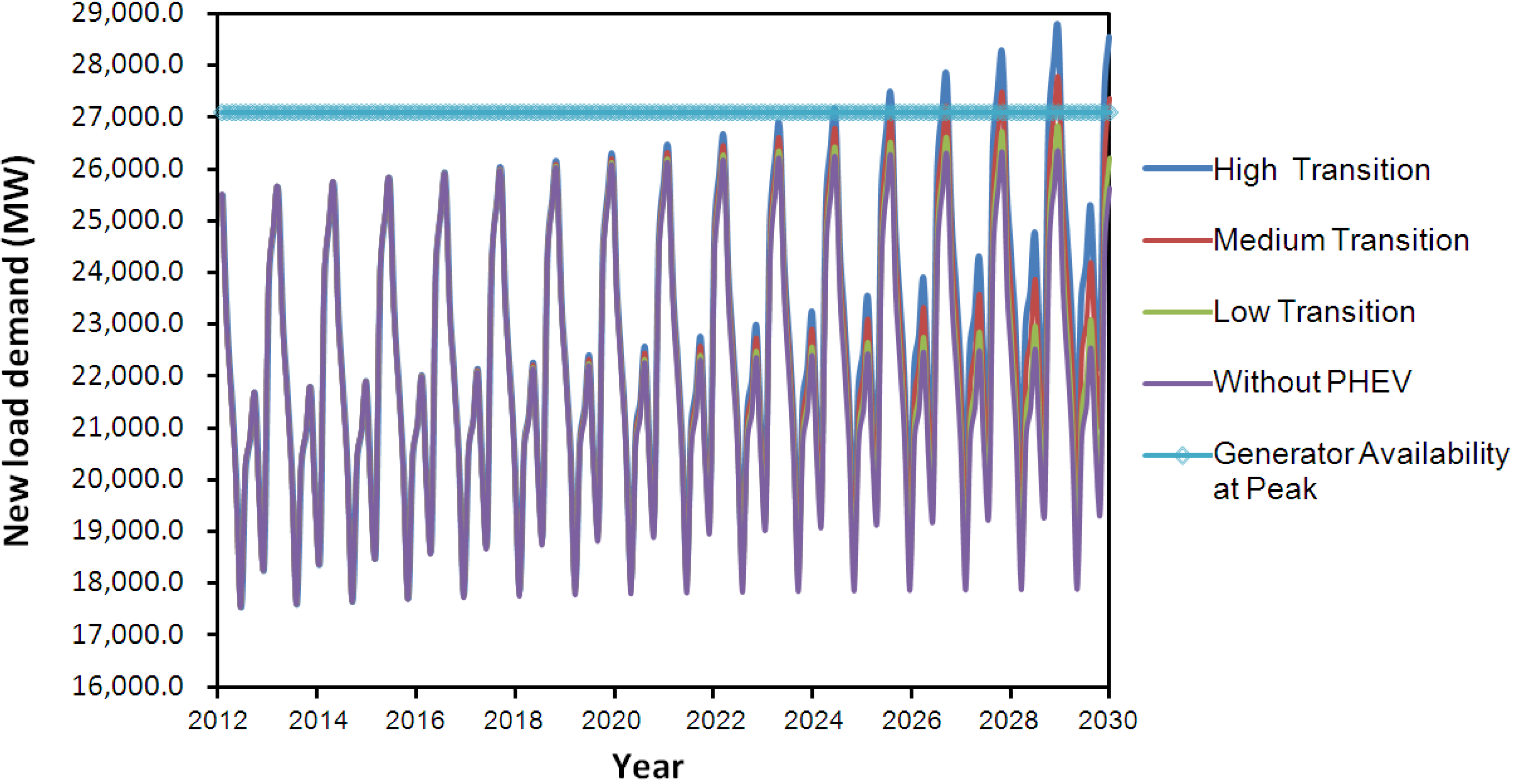
9. Comparisons of Highest Transition with Scenario P100 with Ontario’s Available Resources

Values of all transitions with 10%, 30% and 50% of PHEVs penetration in December 2030 and all scenarios for end of each year from 2012 to 2030 are indicated in Table 7. High transition on Scenario P100, in which all PHEVs are assumed to be recharged in peak period, has the highest value. All transitions and Scenario P100 are selected as the case study to compare with Ontario’s generator availability at peak. As illustrated in Figure 7, in the beginning of 2012 where there is no PHEVs penetration into the transportation sector, the generator is more than the average peak load demand by about 2228 MW. At the end of 2030 in which the total number of PHEVs is 890,362 vehicles per highest transition, peak load demand is greater than the supply by about 1466 MW. Therefore, it can be concluded that available resources in Ontario cannot afford the increasing demand from charging PHEVs between 2012 and 2030. In addition, since Ontario exports electricity to nearby province and USA, the increasing amount from PHEVs charging can reduce the quantity of electricity exported from Ontario.

Figure 7. Comparisons of peak load demand with generator availability at peak in Ontario.

Figure 7. Comparisons of peak load demand with generator availability at peak in Ontario.

Table 7. Peak load prediction of all scenarios and transitions at end of each Year (MW).

Year	Low_P100	Low_P50	Low_P75	Low_P25	Low_P0	Med_P100	Med_P50	Med_P75	Med_P25	Med_P0	High_P100	High_P50	High_P75	High_P25	High_P0
2012	24872	24872	24872	24872	24872	24872	24872	24872	24872	24872	24872	24872	24872	24872	24872
2013	24962	24962	24962	24962	24961	24964	24964	24963	24962	24961	24966	24965	24964	24963	24961
2014	25048	25047	25046	25046	25045	25056	25053	25050	25047	25045	25063	25058	25054	25049	25045
2015	25131	25129	25127	25124	25122	25148	25142	25135	25129	25122	25166	25155	25144	25133	25122
2017	25211	25207	25203	25198	25194	25246	25233	25220	25207	25194	25280	25259	25237	25216	25194
2018	25282	25275	25267	25260	25252	25342	25319	25297	25275	25252	25402	25364	25327	25290	25252
2019	25354	25342	25330	25318	25306	25449	25414	25378	25342	25306	25545	25485	25425	25366	25306
2020	25428	25410	25392	25374	25356	25571	25517	25464	25410	25356	25714	25625	25535	25446	25356
2022	25505	25480	25454	25429	25403	25710	25633	25556	25480	25403	25915	25787	25659	25531	25403
2023	25587	25552	25517	25481	25446	25869	25763	25657	25552	25446	26151	25974	25798	25622	25446
2024	25670	25623	25575	25528	25481	26046	25905	25764	25623	25481	26423	26187	25952	25717	25481
2025	25759	25698	25637	25575	25514	26250	26066	25882	25698	25514	26740	26434	26127	25821	25514
2027	25857	25779	25701	25623	25545	26483	26248	26014	25779	25545	27109	26718	26327	25936	25545
2028	25965	25867	25769	25671	25573	26749	26455	26161	25867	25573	27532	27043	26553	26063	25573
2029	26082	25961	25840	25719	25599	27049	26687	26324	25961	25599	28017	27412	26808	26203	25598
2030	26211	26064	25917	25770	25622	27389	26947	26505	26064	25622	28566	27830	27094	26358	25622

Table 7. Peak load prediction of all scenarios and transitions at end of each Year (MW).

Year	Low_P100	Low_P50	Low_P75	Low_P25	Low_P0	Med_P100	Med_P50	Med_P75	Med_P25	Med_P0	High_P100	High_P50	High_P75	High_P25	High_P0
2012	24872	24872	24872	24872	24872	24872	24872	24872	24872	24872	24872	24872	24872	24872	24872
2013	24962	24962	24962	24962	24961	24964	24964	24963	24962	24961	24966	24965	24964	24963	24961
2014	25048	25047	25046	25046	25045	25056	25053	25050	25047	25045	25063	25058	25054	25049	25045
2015	25131	25129	25127	25124	25122	25148	25142	25135	25129	25122	25166	25155	25144	25133	25122
2017	25211	25207	25203	25198	25194	25246	25233	25220	25207	25194	25280	25259	25237	25216	25194
2018	25282	25275	25267	25260	25252	25342	25319	25297	25275	25252	25402	25364	25327	25290	25252
2019	25354	25342	25330	25318	25306	25449	25414	25378	25342	25306	25545	25485	25425	25366	25306
2020	25428	25410	25392	25374	25356	25571	25517	25464	25410	25356	25714	25625	25535	25446	25356
2022	25505	25480	25454	25429	25403	25710	25633	25556	25480	25403	25915	25787	25659	25531	25403
2023	25587	25552	25517	25481	25446	25869	25763	25657	25552	25446	26151	25974	25798	25622	25446
2024	25670	25623	25575	25528	25481	26046	25905	25764	25623	25481	26423	26187	25952	25717	25481
2025	25759	25698	25637	25575	25514	26250	26066	25882	25698	25514	26740	26434	26127	25821	25514
2027	25857	25779	25701	25623	25545	26483	26248	26014	25779	25545	27109	26718	26327	25936	25545
2028	25965	25867	25769	25671	25573	26749	26455	26161	25867	25573	27532	27043	26553	26063	25573
2029	26082	25961	25840	25719	25599	27049	26687	26324	25961	25599	28017	27412	26808	26203	25598
2030	26211	26064	25917	25770	25622	27389	26947	26505	26064	25622	28566	27830	27094	26358	25622

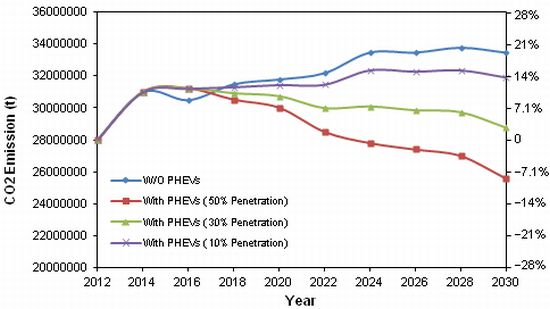
10. Carbon Dioxide Emissions through Highest Transition with Scenario P100

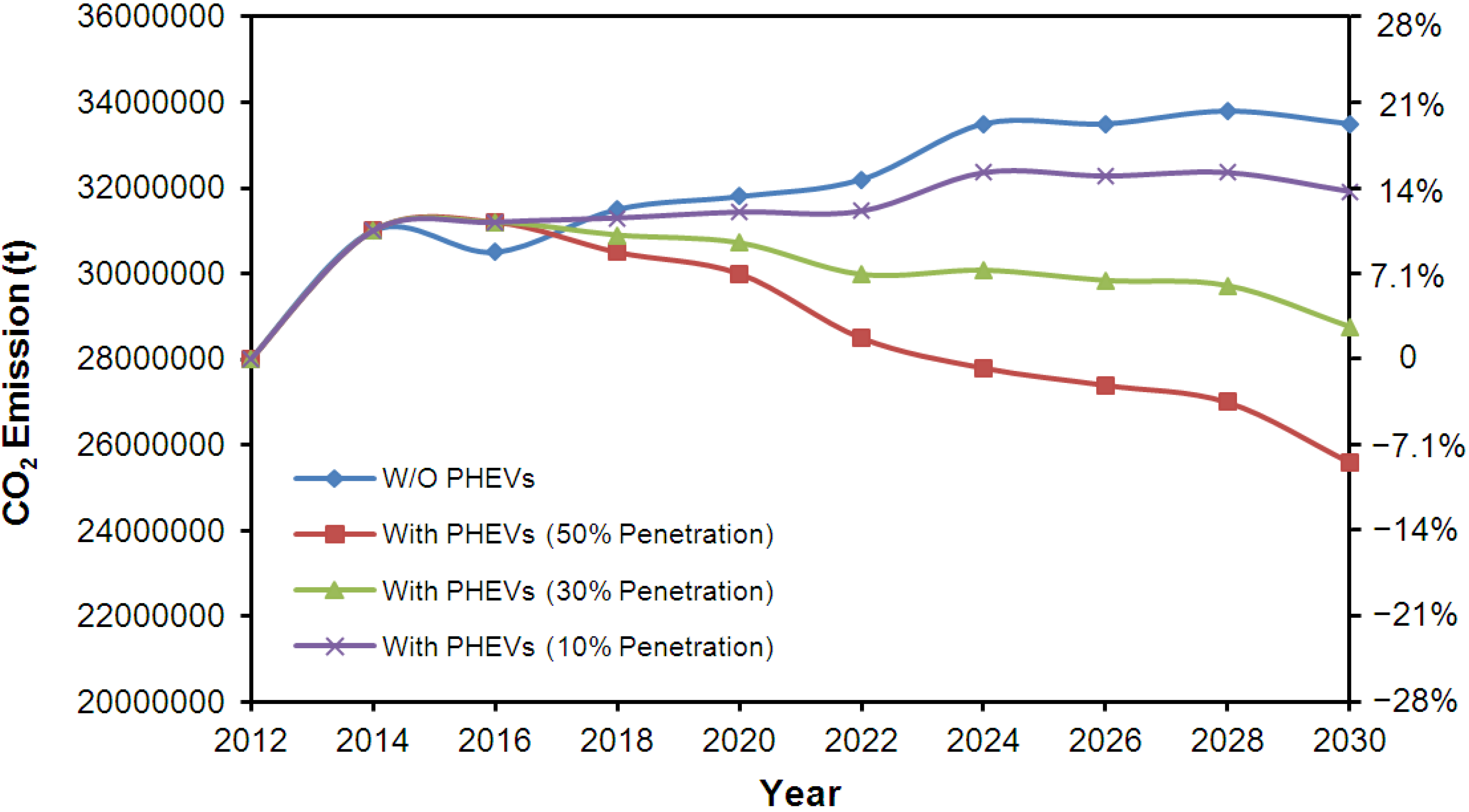
Using PHEVs instead of conventional vehicles causes reduction in total emissions. However, by generating more electricity to satisfy the new demand some part of the emissions reduction would be shifted to the power stations. When considering PHEVs, the total CO₂ emissions over 18 years is found to be 754 Mt, which is 32% less than without PHEVs. Figure 8 shows that there is a small decrease in CO₂ emissions after 2014, because all of coals will be out of service by the end of 2014. Because of the few number of PHEVs in the first 4–5 years, the effect of PHEV penetration start being more noticeable from the year 2018.

Figure 8 also shows the CO₂ emissions for different penetration scenarios. For penetration below 10% level, the CO₂ emissions, although lower than without PHEV, continue to grow over time, reaching a 14% increase in 2030 relative to 2012 emissions. In order for the 2030 CO₂ emissions to be similar to those in 2012, at least 30% penetration level by then is necessary. PHEV penetration level of 50% allows for about 8% reduction in CO₂ emissions in 2030 compared to 2012. Trendwise, penetration level 30% and above allows for a decrease in CO₂ emissions over the year past 2018, whereas for a penetration level of 10% or less, the CO₂ emissions continue to increase.

Figure 8. Carbon Dioxide emission during 2012 and 2030 considering PHEV penetration.

Figure 8. Carbon Dioxide emission during 2012 and 2030 considering PHEV penetration.

11. Conclusions

PHEVs have the potential to penetrate Ontario’s transportation sector in the near future. They can impact the electricity grid if a greater number of PHEVs is recharged to the grid at the same period. Since planning and increasing capacity of existing power plants or even constructing new power plants takes many years to complete, long-term peak and base load forecast models are developed. Also, long-term forecast of the number of light-duty vehicles sold is necessary to see how many PHEVs can penetrate the transportation sector. LR and NLR techniques are employed as forecast techniques to study the relationship between explanatory variables and forecast variables. Weather, demographics, and economic variables are explanatory variables that can impact forecast models. It was found that both the temperature and the GDP have greater impact on peak and base load demands in the winter and the summer. For peak and base loads in the spring and the autumn, they depend only on the GDP. Likewise, GDP is the only factor that has an impact on the number of light-duty vehicles sold. Comparing between LR and NLR by MAE, it was found that NLR most accurately describes peak and base load demands in all seasons except for the base load demand in the winter. Moreover, for light-duty vehicles sold forecast, the LRM has lower errors than the NLRM. However, the differences in the error of both regression models of base load demand in the winter and light-duty vehicles sold are relatively small.

Most accurate regression models which have the lowest MAEs are chosen to project peak and base load demands and the number of light-duty vehicles sold from 2012 to 2030. Three different transitions of PHEVs penetration levels for light-duty vehicles are developed to study the effects of these levels on the electricity grid. By assuming that all PHEVs are recharged during the peak period, high transition whose penetration of PHEVs into the light-duty vehicles in December 2030 is 50% has the highest peak load demand. Additional peak load demands in December 2030 from PHEVs charging in low, medium and high transitions are 210.3 MW, 630.8 MW, and 1051.3 MW, respectively. Five different scenarios of the charging pattern are developed since not all people charge their PHEVs during the off-peak period. By assuming high transition of PHEVs penetration, Scenario P100 has the highest peak load demand, whereas Scenario P0 has the highest base load demand. Additional peak load demands in December 2030 from PHEVs charging in Scenario P100 to Scenario P0 are 1051.3 MW, 788.5 MW, 525.7 MW, 262.8 MW, and 0 MW, respectively. Also, additional base load demand in December, 2030 from PHEVs charging in Scenario P100 to Scenario P0 is 0 MW, 20.9 MW, 41.7 MW, 62.6 MW, and 83.5 MW, respectively.

Finally, the demands for the worse case, assumed highest transition of PHEVs penetration and Scenario P100 of charging pattern, is compared with generator availability at peak in Ontario. It was found that at the end of 2030 in which the total number of PHEVs is 890,362 vehicles, supply is less than the peak load demand by about 1,466 MW. Therefore, it can be concluded that the energy supply sources will not meet future electricity demand of Ontario generating sector for the worst case scenario. Moreover, total emission from to 2012 to 2030 is 754 Mt which is 32% less than without PHEVs in Ontario.