1. Introduction
The increasing electricity demand and price and the concerns about fossil-fueled generation have led to active research to deploy advanced energy systems using distributed generation (DG) sources such as wind, photovoltaic (PV) power, fuel cells (FCs) supported by energy storage system (ESS). These studies have facilitated the use of green energy, thereby reducing energy costs and concerns over the exhaustion of natural resources while curving the carbon emissions.
Stand-alone and grid-connected premise power systems have been proposed to exploit renewable energy sources. The stand-alone system consists only of the DG sources listed above and does not incorporate existing grid power [
1,
2,
3,
4,
5,
6]. This type of system may allow electricity to be provided free-of-charge to consumers once the practical constraints of sizing, siting and environmental concerns are overcome. It is highly expected that the practicality of solar power particularly at the kilowatt scale lowers the barrier to entry and helps more customers adopt it as soon as the parity with retail electricity costs is reached. Note that this paper focuses on the grid-connected residential PV power system and its economic benefits through operation and capital cost for installation is not included for evaluation.
On the other hand, the grid-connected system consists of some renewable DG sources, e.g., PV power tied to the power grid [
7,
8,
9,
10]. Grid-connected systems often reinforced by the ESS seem to be practical for harnessing alternative energy because of the the assurance of a stable power supply. In this system, consumers are required to pay for the grid power and an active energy management plan should thus be beneficial. However, it is interesting to note that existing systems or studies do not incorporate schemes for optimally scheduling the use of grid power and operate rather passively in the following typical way: (1) the system supplies PV-generated power; (2) if there is excess PV power, the system uses it to charge the ESS; (3) if there is no alternative power, the system supplies grid power. This schedule has been considered reasonable in the past because consumers pay for electricity based on consumption, regardless of the time of day. However, several nations plan to start enforcing critical peak pricing, discussed in [
11], or real-time pricing, thus these variables need to be incorporated into the grid-connected system.
Thus, we propose a grid-connected system under time-based rate program such as critical peak pricing (CPP). This system consists of a PV, a battery and grid power. The PV provides renewable energy and is the primary power source of the system while the battery is used for energy storage. Grid power is assumed to be always available, thus guaranteeing the stability of the electrical power supply. We also develop a practical load forecasting method to predict and correlate the power usage with the changing electricity prices (peak pricing periods). This method is based on a new model considering historic load profile, weather and the number of people in a household with a Kalman filter approach. Finally, we design a premise energy management scheme with the proposed load forecasting model to control the flow of power among the different system components. The proposed system uses this management scheme to forecast the next day’s load demand for the peak period and enables economic energy use from the PV and battery as well as inexpensive grid power. If there is no power available from PV or battery power, the system automatically relies on the grid power.
The remainder of this paper is organized as follows.
Section 2 describes the configuration and specifications of the proposed system.
Section 3 introduces the load forecasting technique based on a Kalman filter. The energy management scheme with load forecasting is discussed in
Section 4.
Section 5 evaluates the performance of the proposed system for several practical operating scenarios and demonstrates its economic benefits. Conclusions are presented in
Section 6.
2. System Configuration and Specification
2.1. System Configuration
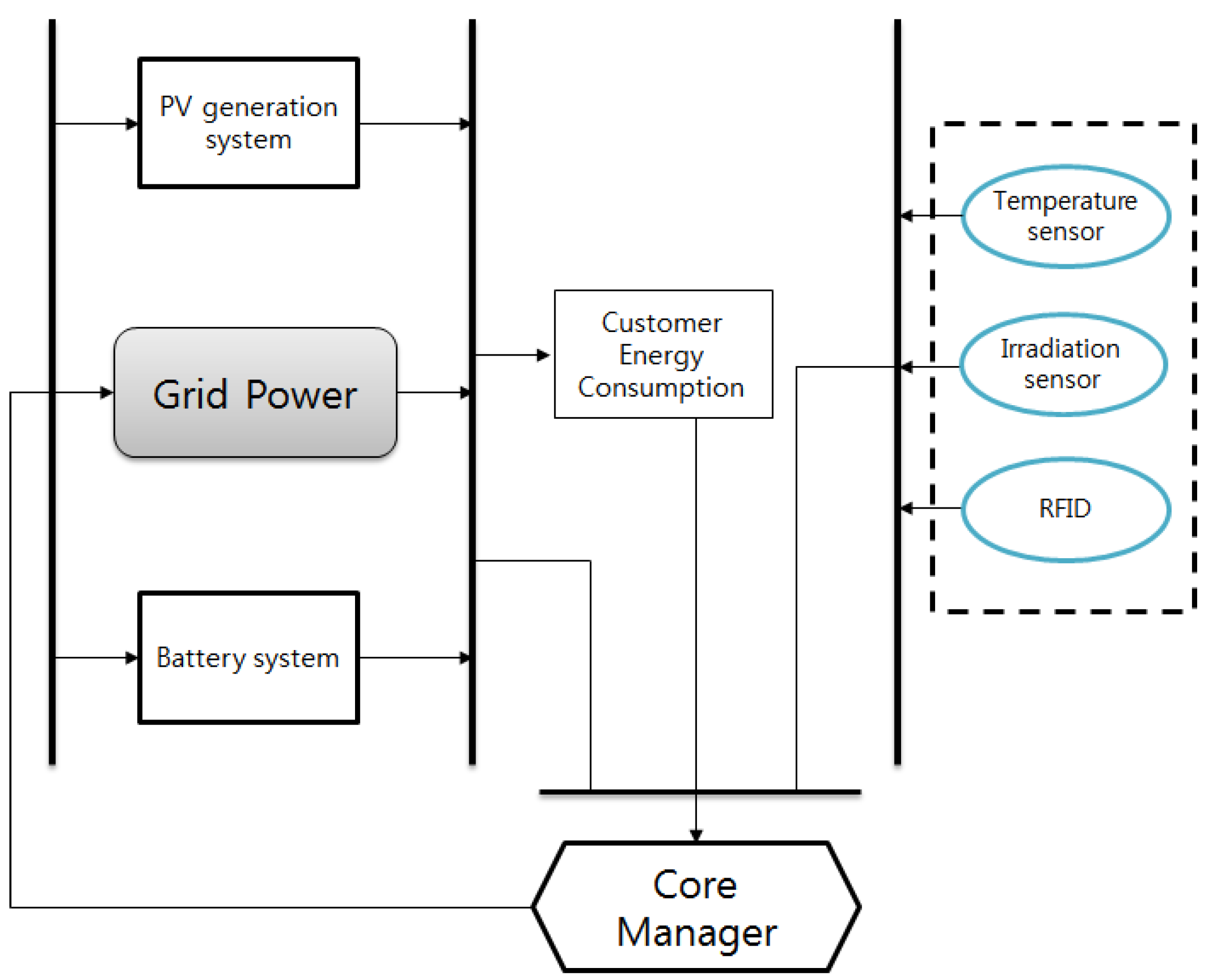
Figure 1.
Configuration of the proposed premise energy management system.
Figure 1.
Configuration of the proposed premise energy management system.
The configuration of the proposed grid-connected system is shown in
Figure 1. This research assumes that the system consists of a 1-kW (peak) PV array as the primary energy source, which is controlled by a maximum power point tracking (MPPT) controller, a battery for storing extra or inexpensive power, and may use the grid power under critical peak pricing to ensure a stable supply of electricity through 220 V/60 Hz link in Korea. This grid connection guarantees high reliability, modularity and scalability of a hybrid system [
12]. The PV array with battery system and the grid can be seamlessly integrated with advancing power electronics. Modern power converters are highly efficient in that the efficiency becomes over 95% and thus converter losses are not considered in this research. The system is further assumed to be equipped with weather and RFID (Radio Frequency Identification) sensors for obtaining information on temperature, solar irradiation and the number of people in the household [
13]. A core manager (CM) is designed for determining the power flows in the system by using the load forecast and the power from the PV and monitoring the state of charge (SOC) of the battery. Losses occurring during charing and discharging are not included in this research. The CM commands the system components accordingly and dictates whether PV power, battery power or grid power is consumed at the current operating time. The CM effectively manages the battery power. For example, when there is any more PV power than is required, the CM monitors the SOC of the battery and starts charging the battery as needed. When greater power is needed during peak usage while the grid power is economic, the system may start using grid power and even charge the battery for future use.
Table 1 lists the component specifications of the proposed grid-connected system assumed to be deployed in a typical residential premise (
Figure 2). In this research, we consider a widely used PV model as represented in Equation (
1), where
G is the incident irradiance,
is the maximum output power and
T is the temperature.
,
and
are the maximum reference power, the reference incident irradiance and temperature respectively, and
γ refers to the maximum power correction factor for temperature [
14].
Table 1.
System components specifications.
Table 1.
System components specifications.
| Components | Specification |
|---|
| Photovoltaic Array | Maximum reference power = 1 kW,
= 25 °C, = 1000 W/m |
| Battery | Capacity = 0.9 kWh, Charge and Discharge rates are 0.3 and 0.9 kWh/h |
| Grid power | Ready to be connected with 220 V, 60 Hz |
| Sensors | Temperature, irradiation sensors and RFIDs |
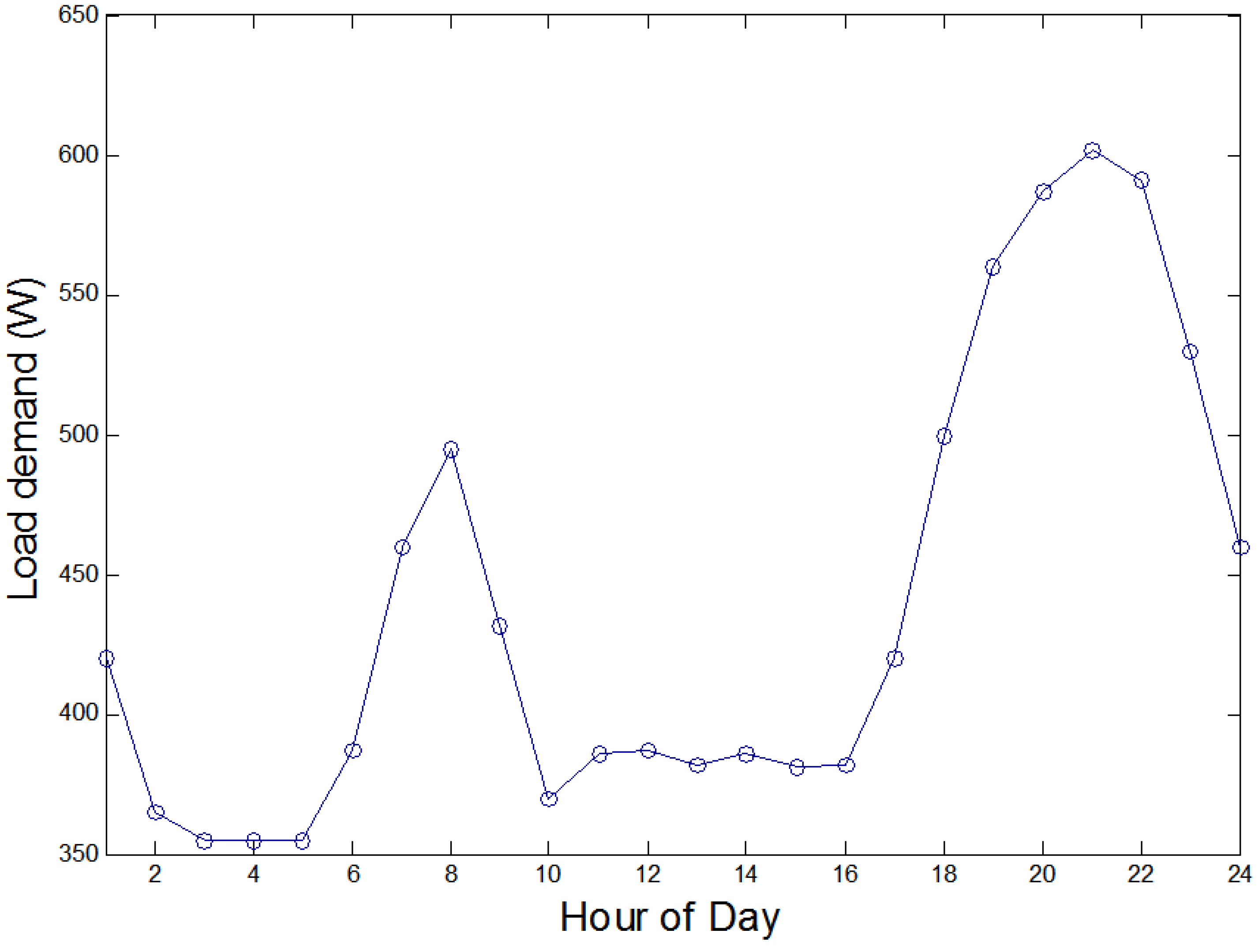
Figure 2.
Sample of hourly electrical demand in Korea.
Figure 2.
Sample of hourly electrical demand in Korea.
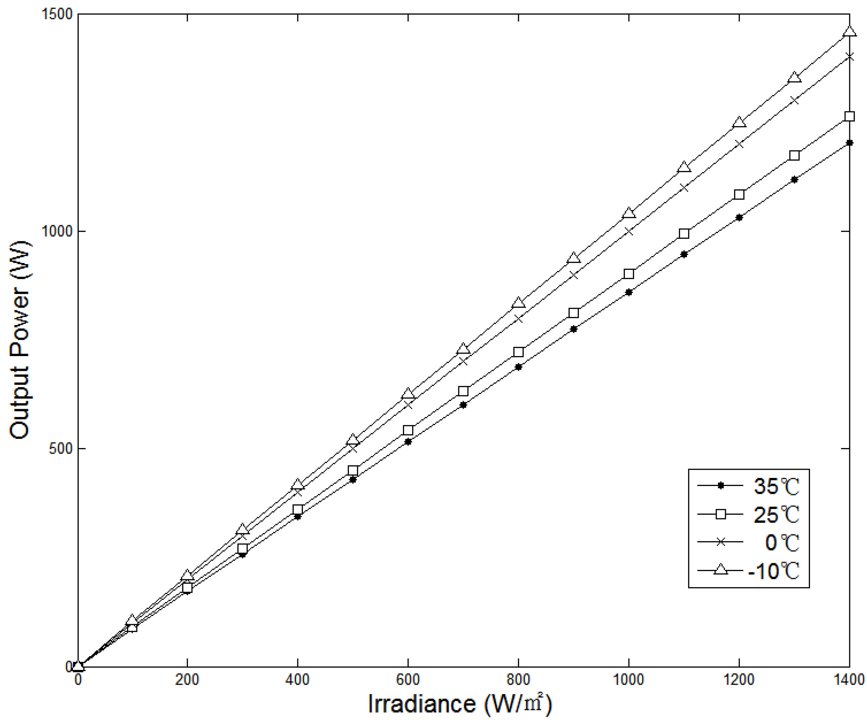
The PV generating power along with varying irradiance and temperature is also illustrated in
Figure 3. It manifests that higher irradiance results in larger output power of the PV array. Conversely, the maximum power decreases with increasing temperature. In this research, it is assumed that PV keeps providing the same power output for one hour for the convenience of demonstrating the economic benefit in terms of cost per kWh.
The performance of the battery system for storing excess PV power or inexpensive grid power in preparation for the peak pricing period may depend on its size but a 0.9 kWh-ESS (90% of the maximum PV power) is adopted in this paper. This battery is specified to have a 0.3 kW per hour charge rate and a 0.9 kW per hour discharge rate. Finally, useful sensors are assumed to be installed in the system for collecting data such as temperature, irradiation and the number of people in the house as used in the core manager and load forecasting scheme.
Figure 3.
The output power characteristics of a PV array under different irradiance intensities and temperatures.
Figure 3.
The output power characteristics of a PV array under different irradiance intensities and temperatures.
3. Load Forecasting Based on Kalman Filter
Securing the proper amount of premise power during the peak period in a CPP market is the key to the proposed energy management system. Thus, this research incorporates load forecasting to inform the amount of necessary power and proposes a new load model taking into consideration the number of people in the house at the operating hour. Since there are many controllable electrical appliances that can be turned on or off in a modern household (e.g., computers, air conditioner, washing machine, TV, etc.), it is important to consider the number of people in the house in predicting the load demand.
3.1. Load Model
One of the most important tasks in forecasting load demand is to develop an appropriate load model because it determines the prediction accuracy. Neural networks and parametric based methods may be two well-known forecasting approaches [
15,
16,
17]. Commonly used load models include non-weather sensitive models, weather-sensitive models and hybrid models [
18]. One may observe many sophisticated algorithms for improving the forecasting accuracy especially for securing the grid operations. Each curve in
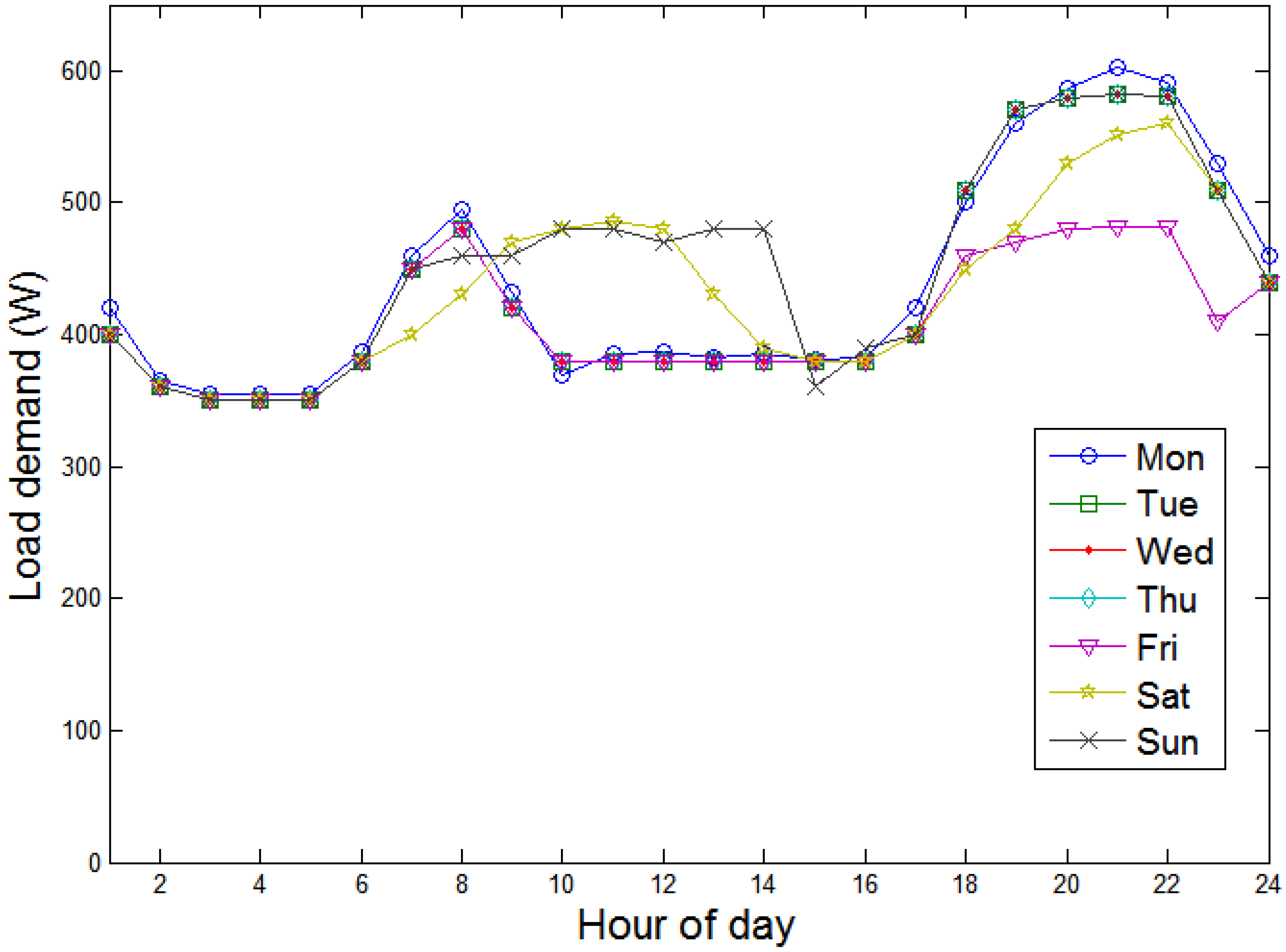
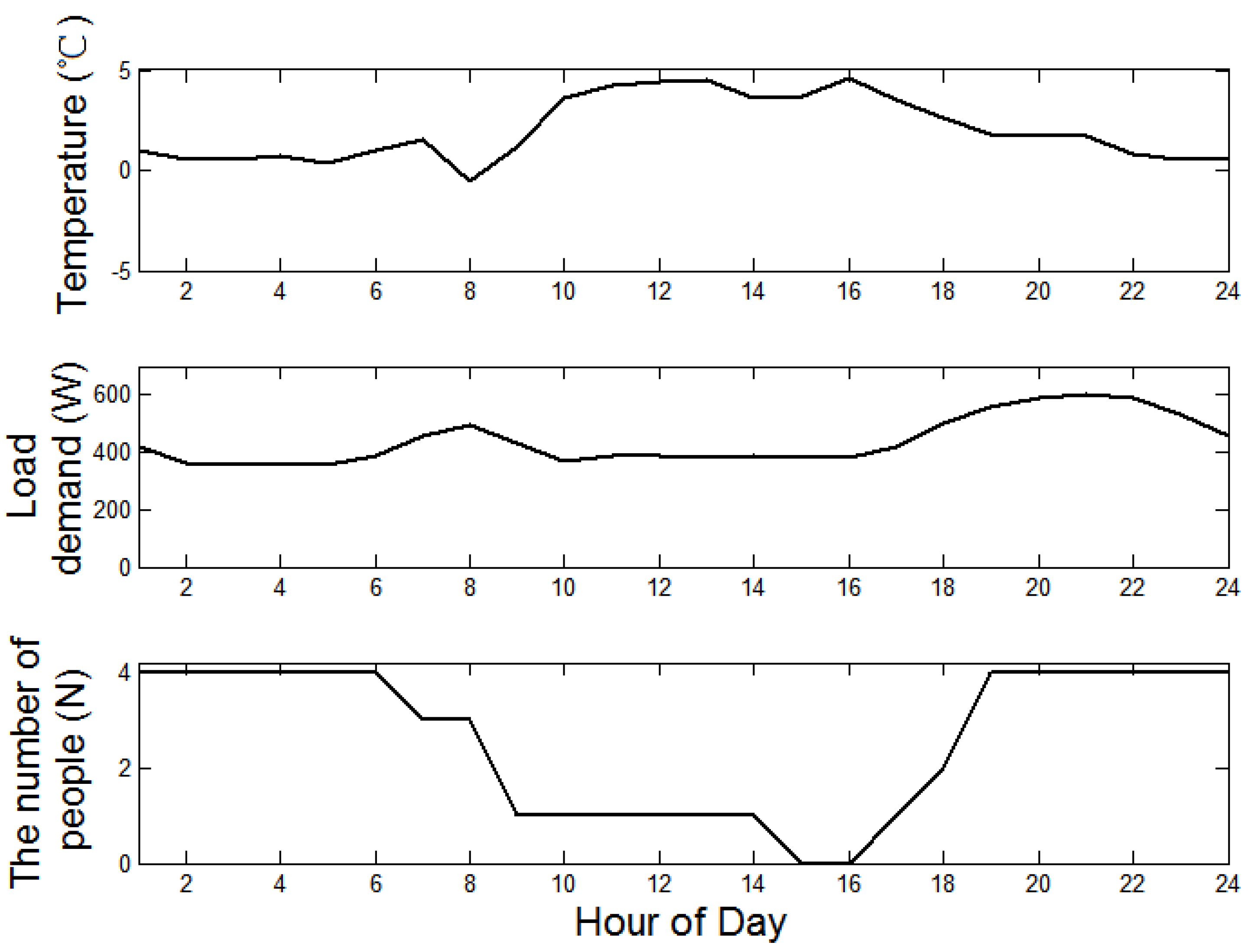
Figure 4 shows actual hourly load demand of a typical Korean household for one day.
Figure 5 illustrates fluctuations in load, temperature and the number of people in the house over the course of a day. It is evident from
Figure 5 that load demand increases as temperature decreases and the number of people in the house increases.
Figure 4.
Daily fluctuations in load for the week.
Figure 4.
Daily fluctuations in load for the week.
Figure 5.
Daily fluctuations in load demand, temperature and the number of people in the house.
Figure 5.
Daily fluctuations in load demand, temperature and the number of people in the house.
Pursuing the practicality of the algorithm, we design a Kalman filter-based parametric model that depends on past load demand, temperature and the number of people in the house as presented below:
where subscripts
n and
indicate an hour of the day and day itself, respectively;
and
.
E,
T and
N are the load, temperature and the number of people in the house, respectively.
corresponds to the load consumption of the previous hour on the same day,
is the load consumption for the same time period a day prior, and
is the load consumption for the same time period a week prior.
T and
N are treated in exactly the same manner.
is a base coefficient at the hour of
n,
are the coefficients of load demand, temperature and the number of people in the house. Every parameter is assumed to remain constant over each discrete time period (one hour). Accordingly, 24 sets of coefficients are required to be estimated for a single day forecasting. However, we use an average of these coefficients in our model in order to minimize the computational complexity. Useful heuristics may be added to reinforce the accuracy of the algorithms to accommodate special occasions or seasonal variations such as the impact of climate change.
3.2. Kalman Filtering
As indicated above, the recursive discrete Kalman filter has been used to estimate parameters of our load model [
19,
20]. Consider the following discrete state equations to develop the load model:
where
is a vector of
system states,
represents the
dimensions of the state transition matrix,
is
measurement vector,
is
output matrix,
is
system error and
is
measurement error. The noise vectors
and
are drawn from white Gaussian noise with zero means and no time correlations as presented below.
Covariance matrices,
and
are also defined as follows:
Given a priori estimate of the state vector
and its error covariance matrix
, we set
and then the Kalman filter algorithm is applied to estimate the next states by recursively computing the following set of equations.
where
is the Kalman gain. In this Kalman filter algorithm, it is important to choose a priori estimate of the state
and its covariance error
because intelligent choice helps increase accuracy and decrease the computational complexity of the algorithm. A few measurement vector samples can be considered as initial values for
and
as presented below:
The discrete state equations in Equations (
3) and (4) are defined for the forecasting model in the following way:
The state transition matrix, , is a constant identity matrix.
The error covariance matrices, and are constant identity matrices.
The state vector,
, has ten parameters based on Equation (
2),
.
The time-varying output matrix, , also has ten parameters derived from the load demand profile, temperature and the number of people in the house.
The observation value,
, represents the load at time
k.
takes the following form as presented in Equation (
13) as was defined in Equation (
2):
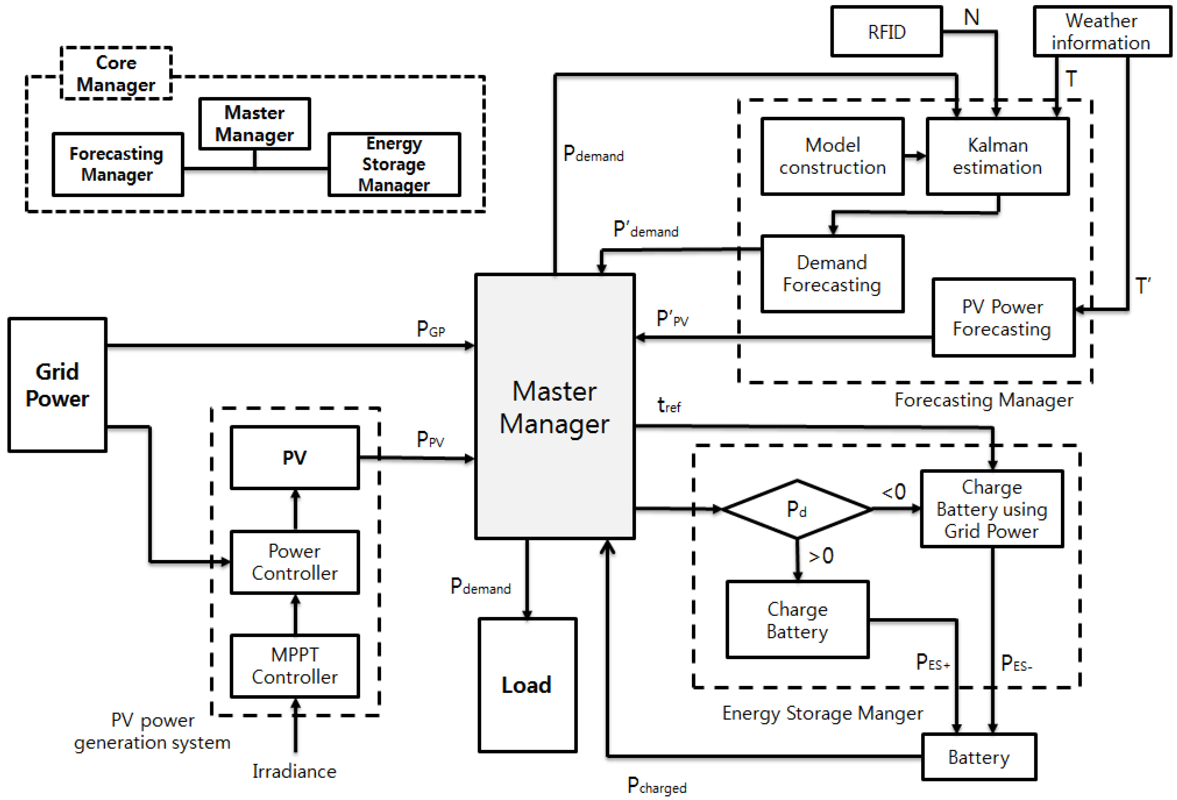
4. Premise Power Management Scheme
Figure 6.
Configuration of the proposed premise energy management system.
Figure 6.
Configuration of the proposed premise energy management system.
In this section, we describe a premise power management scheme (
Figure 6) for effectively controlling the power flows among different energy sources in the residential premise. The power management scheme manages these sources through load forecasting, energy storage and a master manager (MM) in the core manager. The aforementioned load forecasting is implemented in a forecasting manager (FM) and the battery and its controller are located in the energy storage manager (ESM). The MM works with these component managers and controls the generating sources.
The proposed scheme begins with forecasting the amount of load demand and PV generation via the FM. This research has done hourly forecasting but it may be flexibly adjusted to the scanning rate of input data. The FM constructs a load forecasting model as discussed in
Section 3 and informs the MM of the predicted load demand. Additionally, the FM can estimate the amount of PV power by collecting weather information from sensors or a weather forecasting service.
In the next step, the ESM determines the way to charge the battery. It first forecasts power difference between the PV power and power demand based on Equation (
14):
where
is the power difference between the forecasted PV power
and load demand
. Power loss of the converters are ignored for simplicity.
At any given time, if
is positive, the ESM stands by until there is actual excess power to store after the household occupants start using the electricity. The amount of excess PV power to be stored is calculated through the following equation:
where
is excess PV power available,
and
correspond to the PV power being generated and consumed by occupants, respectively. When
, command for securing the power reserve is initiated based on a potential power shortage,
calculated by Equation (
16). A reference time is defined as
, which is set to be three hours prior to the peak time based on battery capacity and charging rate,
i.e., the ESM completes each round of estimation every three-hours ahead of the operating time in this research. And it is at this point that the system begins charging the battery based on
for use during the peak period.
where
is the power stored in the battery before a given time. If
, the battery already has sufficient power to cover a potential shortage and thus does not require a charge using grid power.
In the third step, the MM chooses an energy source among the PV, grid and battery options. It prioritizes the PV as the primary source, but if there is no PV power available and the given operating hour is not within the peak pricing period, the MM uses grid power as the primary source. However, during the peak pricing period, the MM uses battery power first, and then grid power is the last resort if there is no battery power available.
5. Simulation Results
Simulation studies are performed using MATLAB to demonstrate the efficacy of the proposed premise power management system. The electrical cost savings with the proposed system are evaluated with reference to the costs without the proposed scheme. Also the systems are assumed to be deployed in a residential premise where four people live. Actual hourly load data measured from a typical Korean middle-class household is used in this study. The weather data are obtained from the Korea meteorological administration [
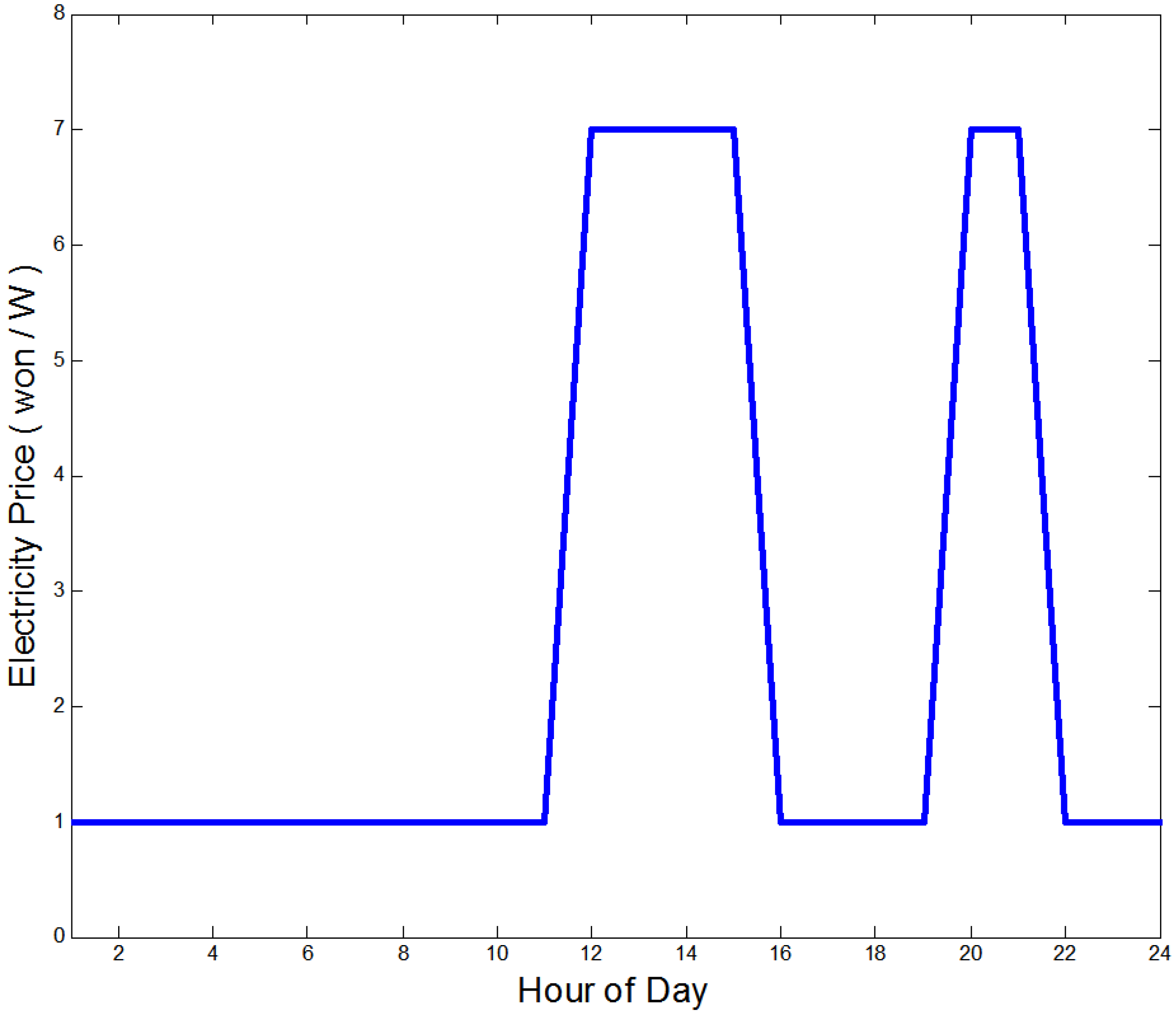
21]. Additionally, the critical peak pricing curve is assumed to have two peaks as presented in
Figure 7.
Figure 7.
An example of a critical peak pricing (CPP) curve.
Figure 7.
An example of a critical peak pricing (CPP) curve.
After a training mode for constructing the load forecasting model, simulations are carried out for evaluating the performance of the power management system under three different scenarios. The first scenario is for a normal situation in which the PV generates the expected amount of power and there is no unexpected load demand. In the second scenario, the forecasting works fine but the PV is unable to generate sufficient power due to unfriendly weather condition. The last scenario considers a forecasting failure so that significant discrepancy between the actual load demand and the forecasted one exists.
5.1. Training Mode to Construct load Forecasting Model
To forecast the load for the next day, initial parameters such as
, a set of
α’s, and
in Equations (
11) and (12) must be defined. In this simulation, we set those parameters arbitrarily. Using these parameters and data for monthly load demands, temperature and the number of people in the house, we run the Kalman filter to estimate values of the load model coefficients (
Table 2).
Table 2.
Estimated coefficients of the proposed forecasting model.
Table 2.
Estimated coefficients of the proposed forecasting model.
| α1 | α2 | α3 | α4 | α5 | α6 | α7 | α8 | α9 | α10 |
|---|
| 0.5962 | 0.2373 | 0.2182 | 0.0559 | 0.2963 | 0.3962 | 0.1912 | 0.1962 | 0.1989 | 0.2991 |
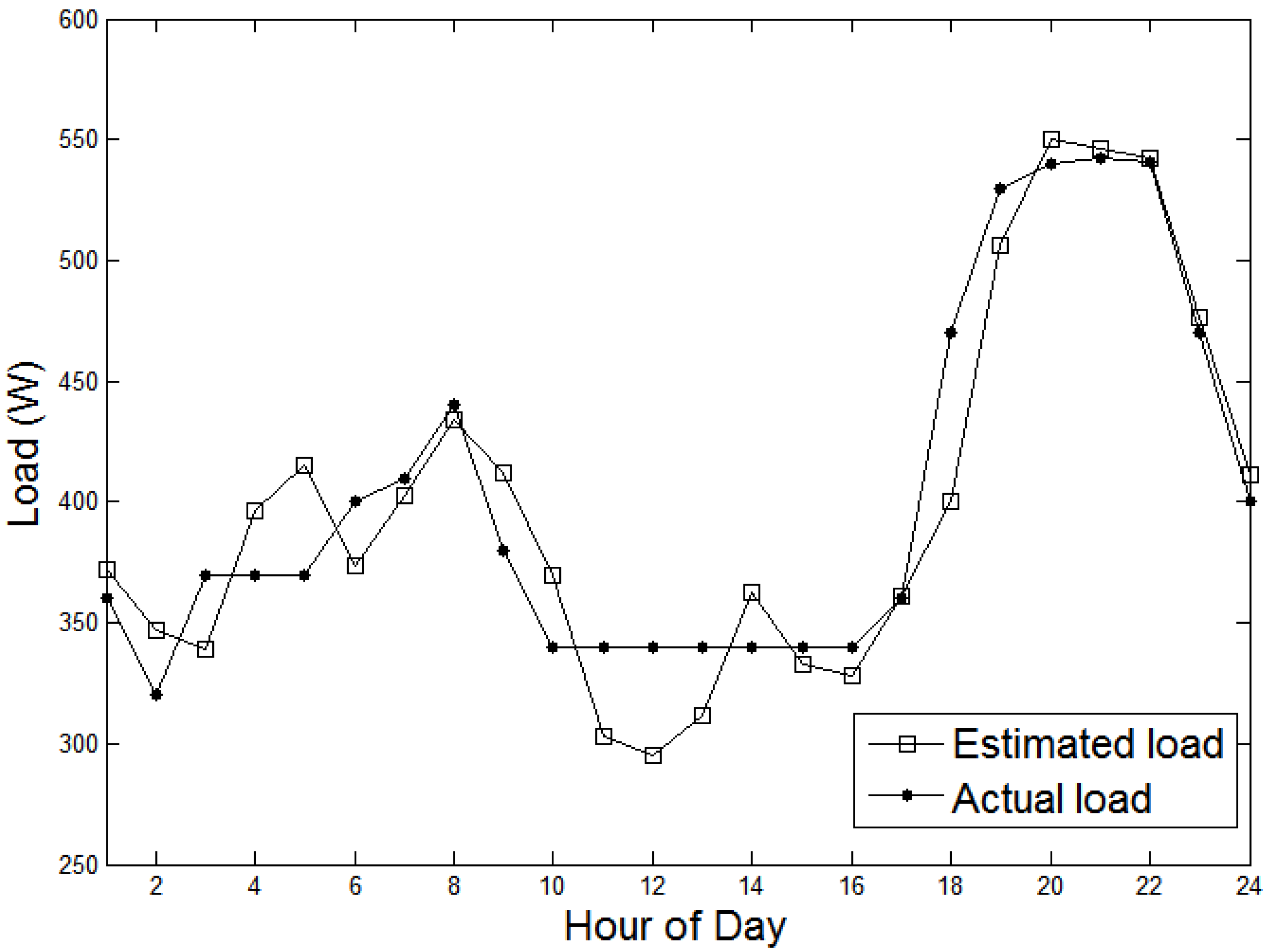
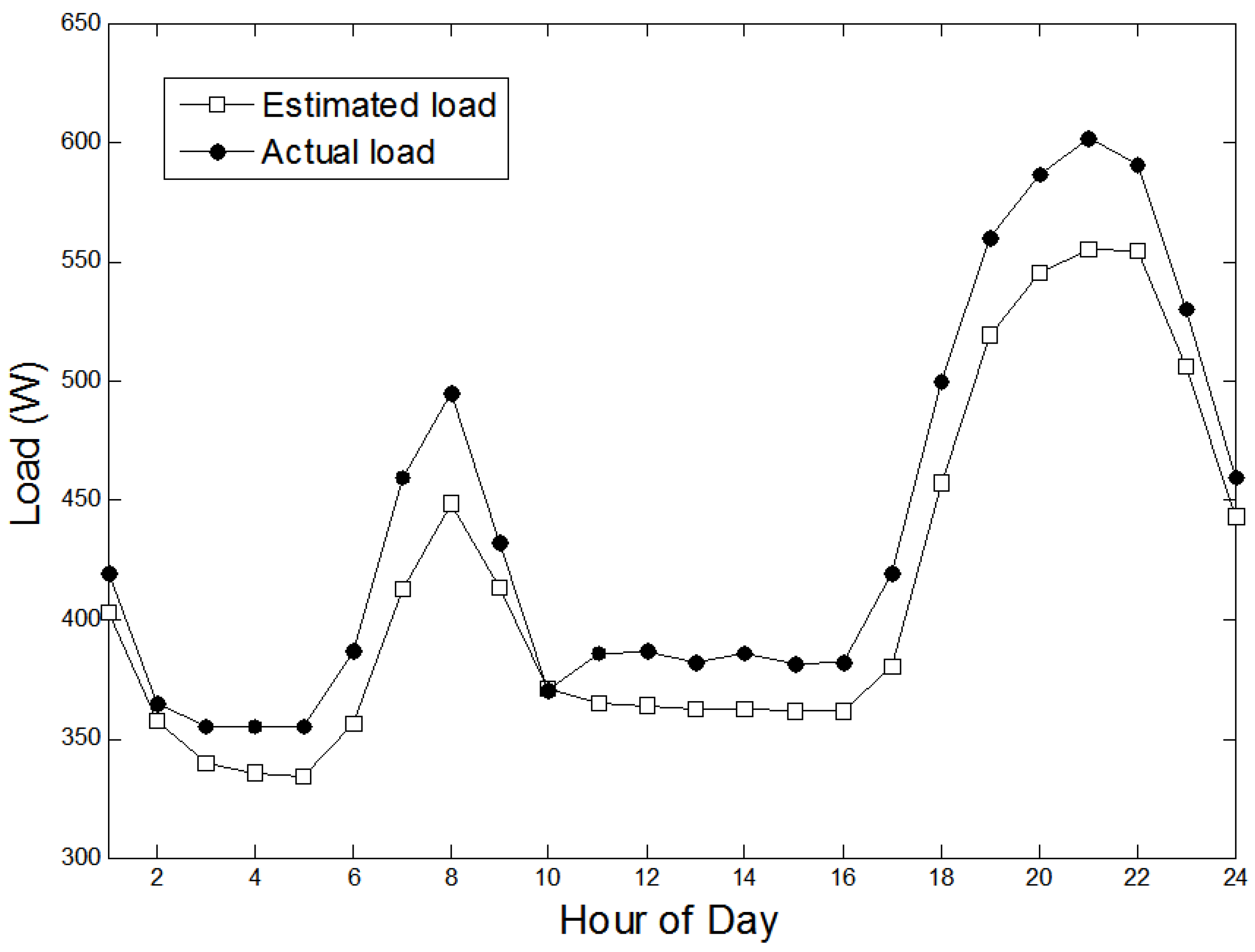
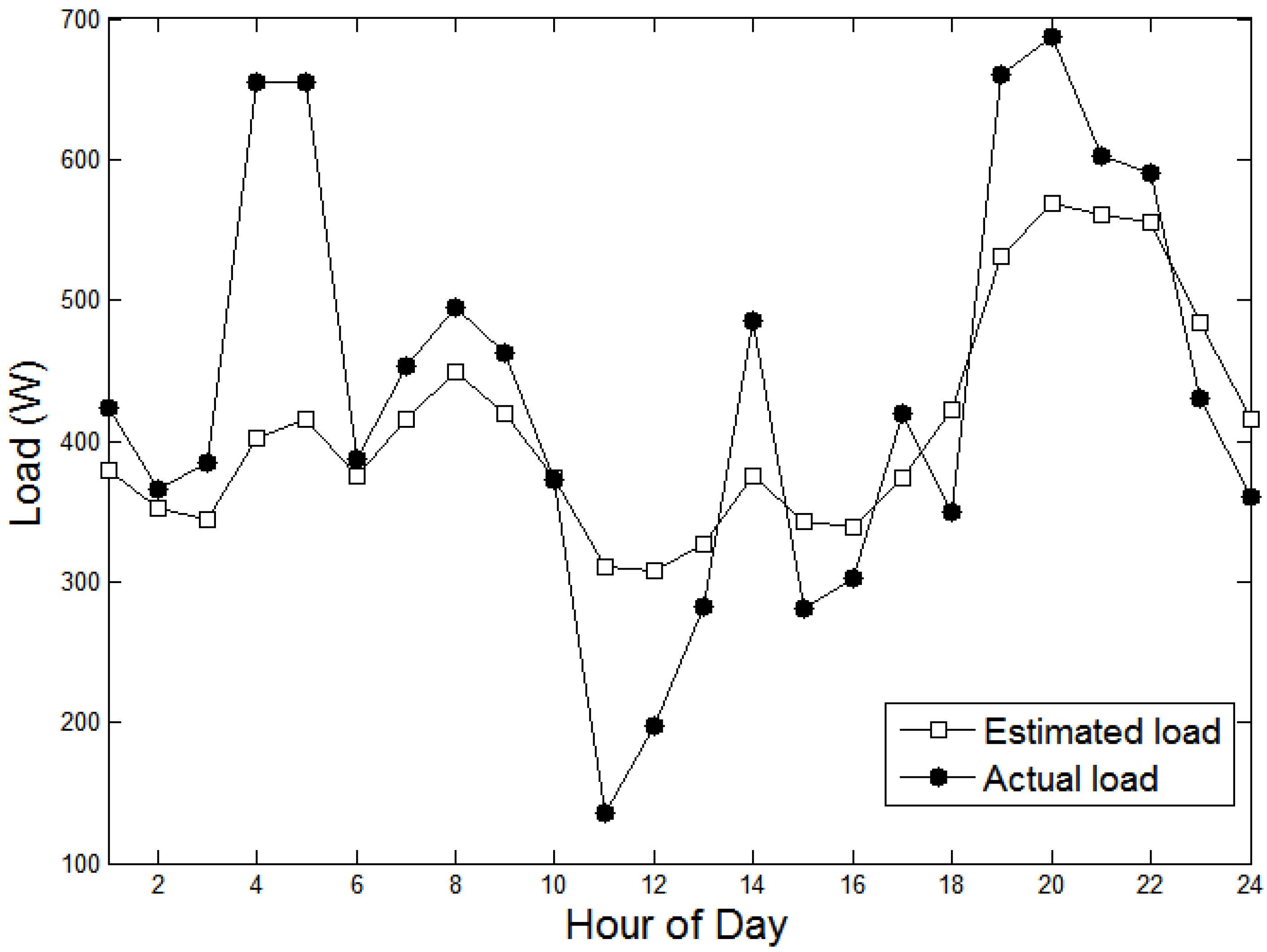
The forecasted load demand using the estimated parameters above is presented in
Figure 8 with reference to the actual load demand, clearly indicating the accuracy of the proposed forecasting model.
Figure 8.
Actual and estimated load demands.
Figure 8.
Actual and estimated load demands.
5.2. Scenario 1
We investigate the scenario 1 using the data in
Figure 9,
Figure 10 and
Figure 11. The hourly power output from the PV is shown in
Figure 12. As assumed in
Section 2, the MPPT controller ensures the maximum power output governed by solar irradiance. It is evident in
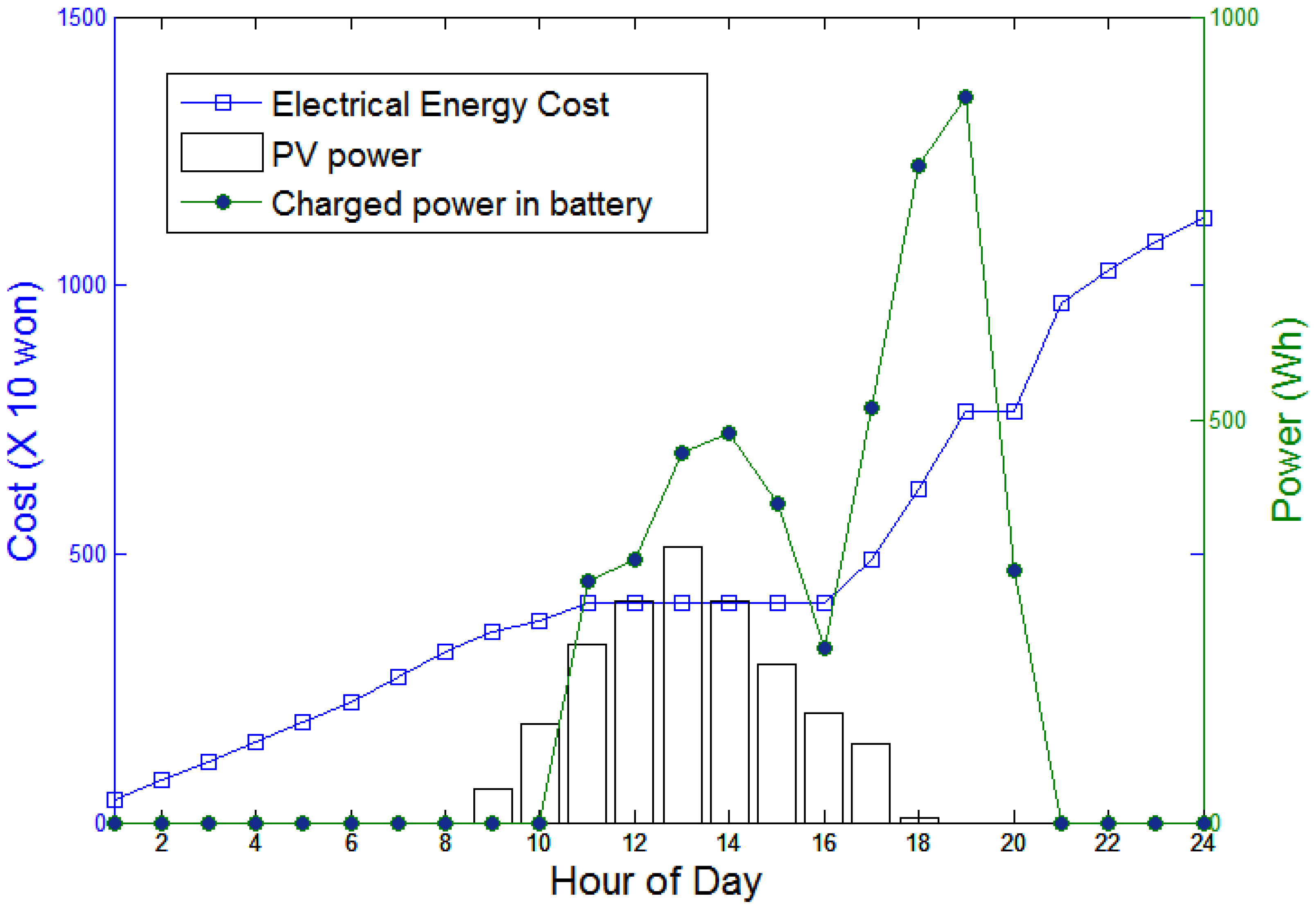
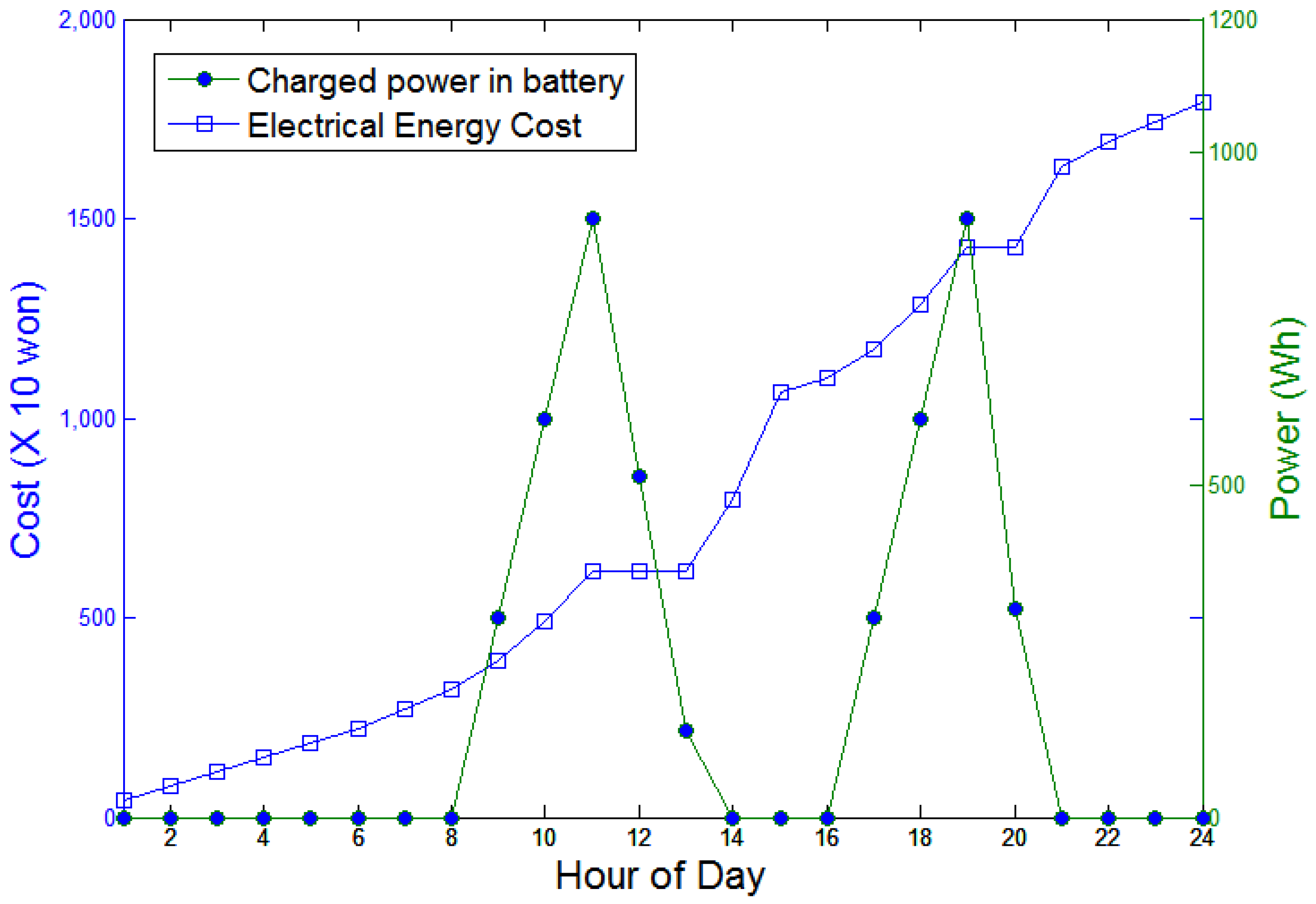
Figure 13 that the FM accurately predicts the load demand. The electricity prices increase in such periods as 1:00–11:00, 16:00–19:00 and 21:00–24:00 because the load demand is greater than the sum of the power generated by the PV and the charged battery (See
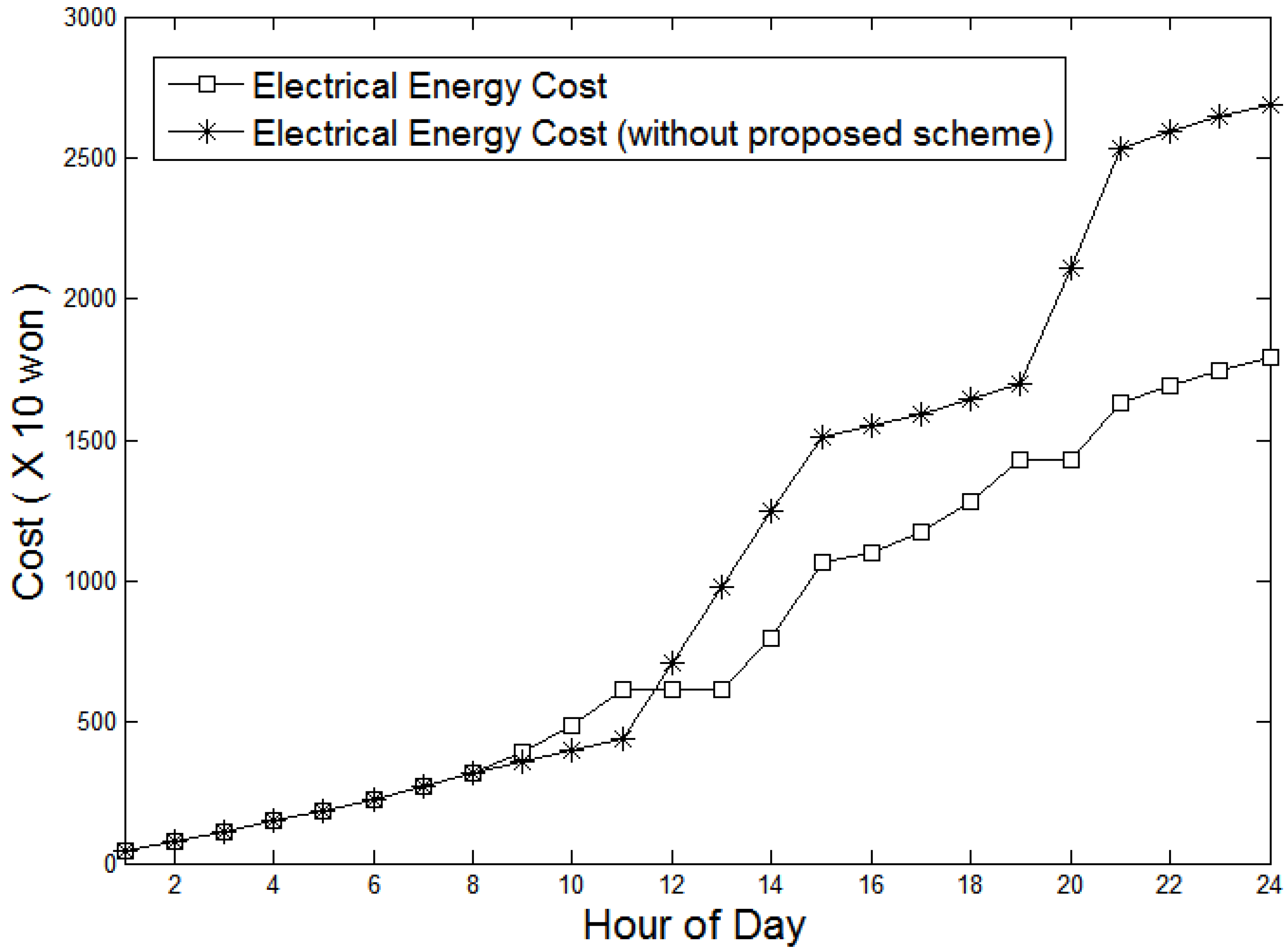
Figure 12). Thus, the occupant should use the grid power during these periods. In contrast, from 11:00 to 14:00, the PV generates power greater than the required and charges the battery with excess PV power. Although the power output from the PV is not sufficient to fully charge the battery, there is no need to use the grid power from 14:00 to 16:00. The electricity price and the SOC of the battery increase sharply between 16:00 and 19:00, indicating that the proposed system begins charging the battery using the grid power in response to a forecasted power shortage during the peak time period of 20:00–21:00. If the system does not charge the battery during that time, the occupants need to pay higher price during the peak usage period (
Figure 14).
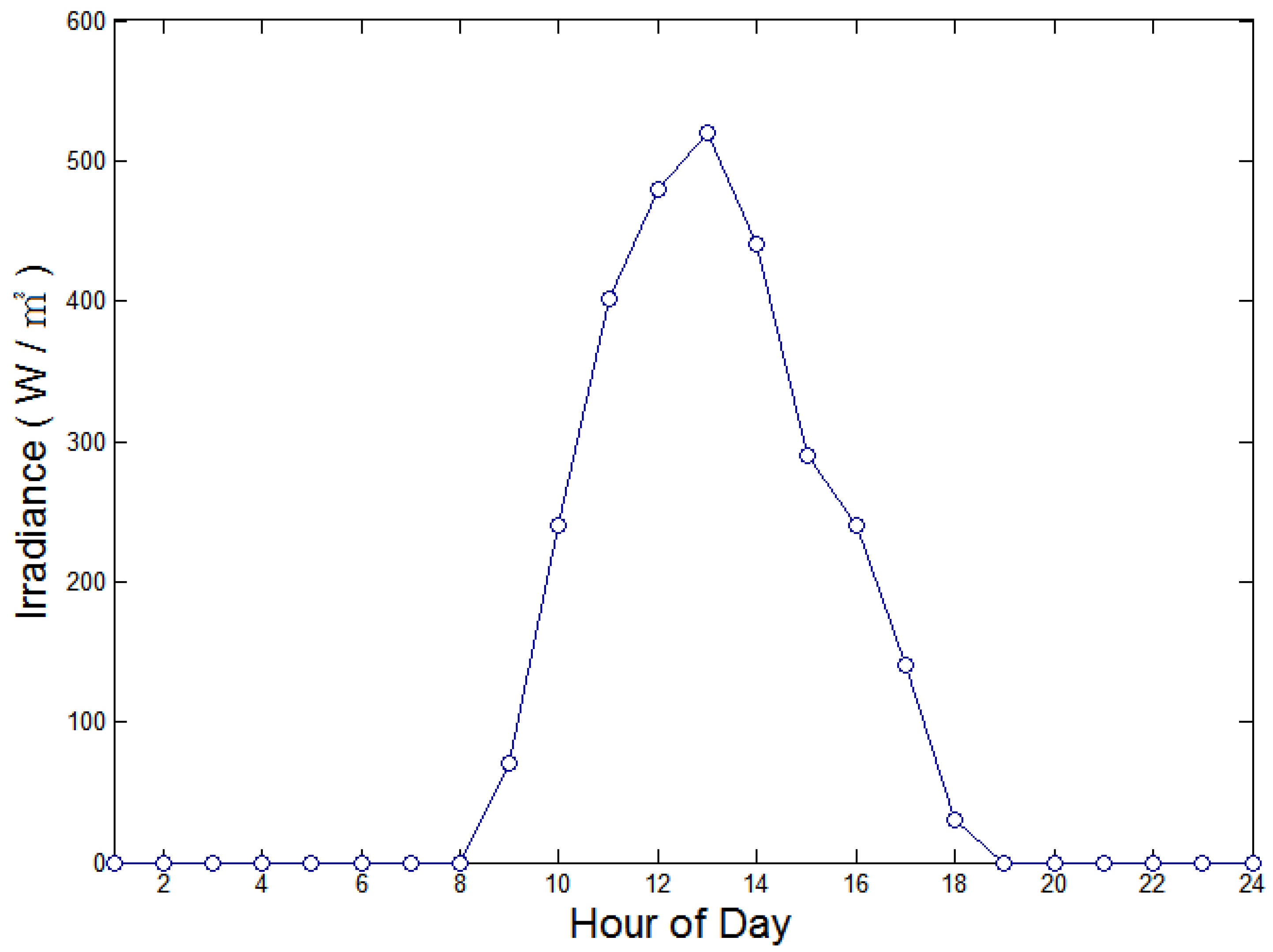
Figure 9.
Daily solar irradiance fluctuations.
Figure 9.
Daily solar irradiance fluctuations.
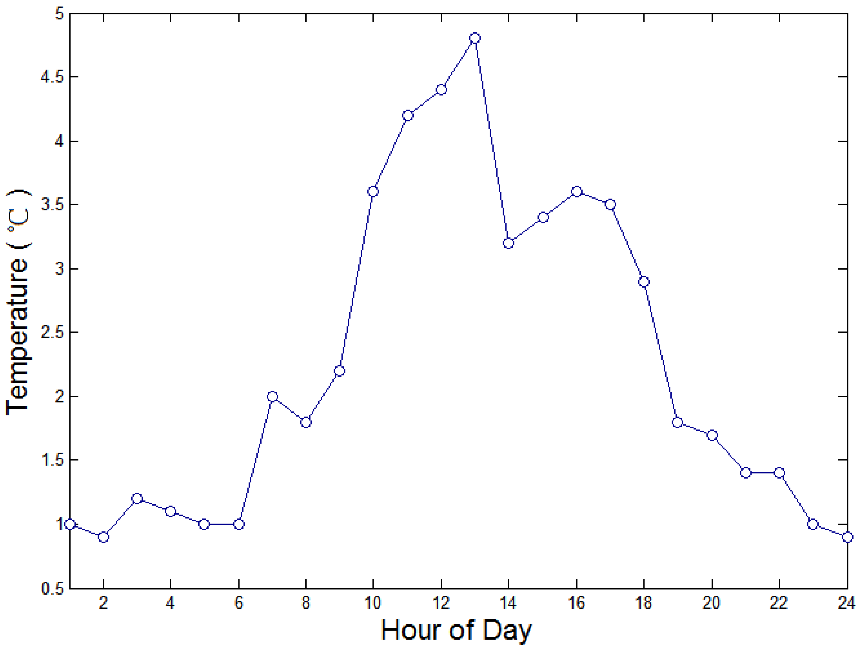
Figure 10.
Daily temperature fluctuations.
Figure 10.
Daily temperature fluctuations.
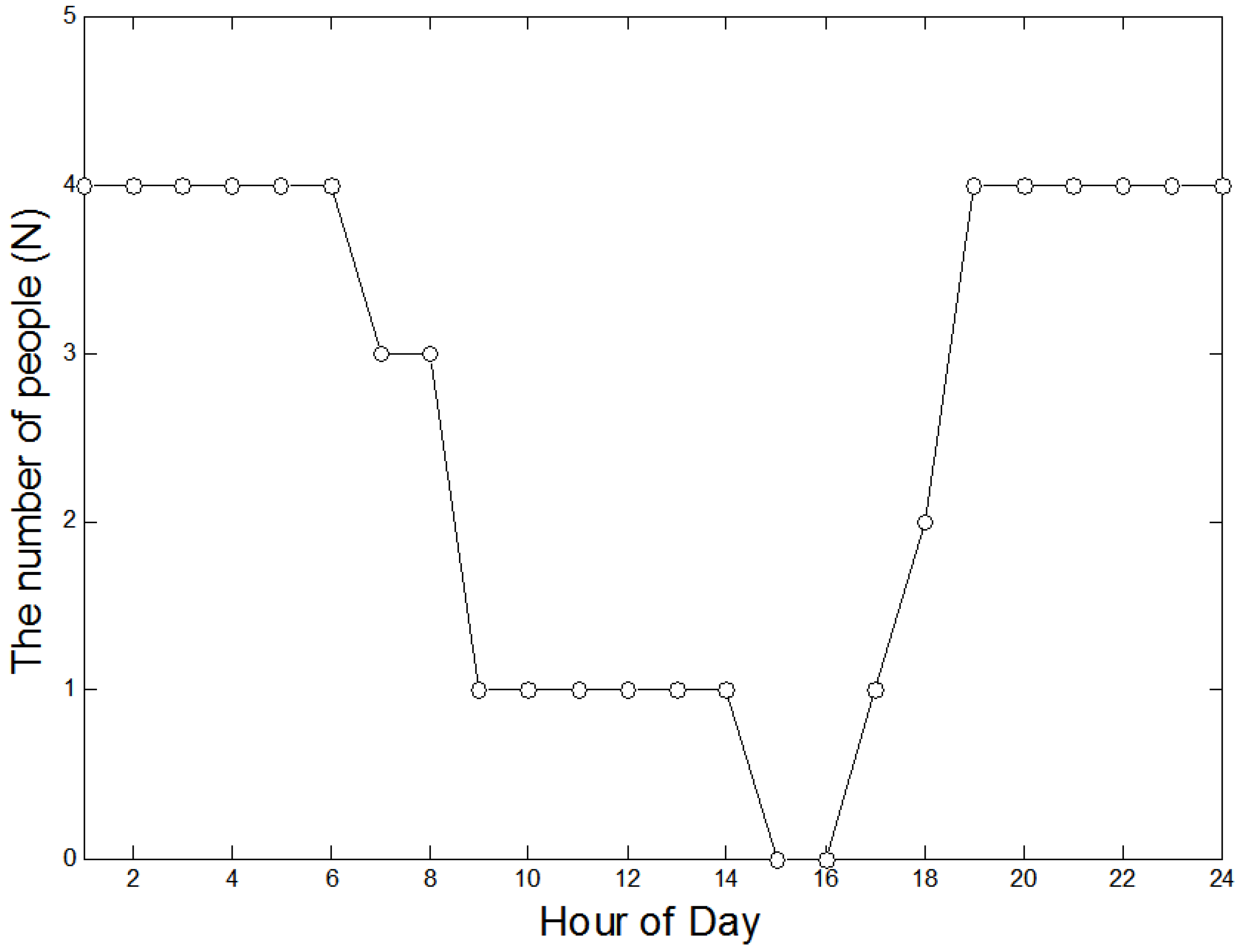
Figure 11.
The number of people in the house over the course of a day.
Figure 11.
The number of people in the house over the course of a day.
Figure 12.
Use of PV power, SOC of the battery and electricity price under Scenario 1.
Figure 12.
Use of PV power, SOC of the battery and electricity price under Scenario 1.
Figure 13.
Actual and estimated load demands for Scenario 1.
Figure 13.
Actual and estimated load demands for Scenario 1.
Figure 14.
Comparison of electricity prices in Scenario 1.
Figure 14.
Comparison of electricity prices in Scenario 1.
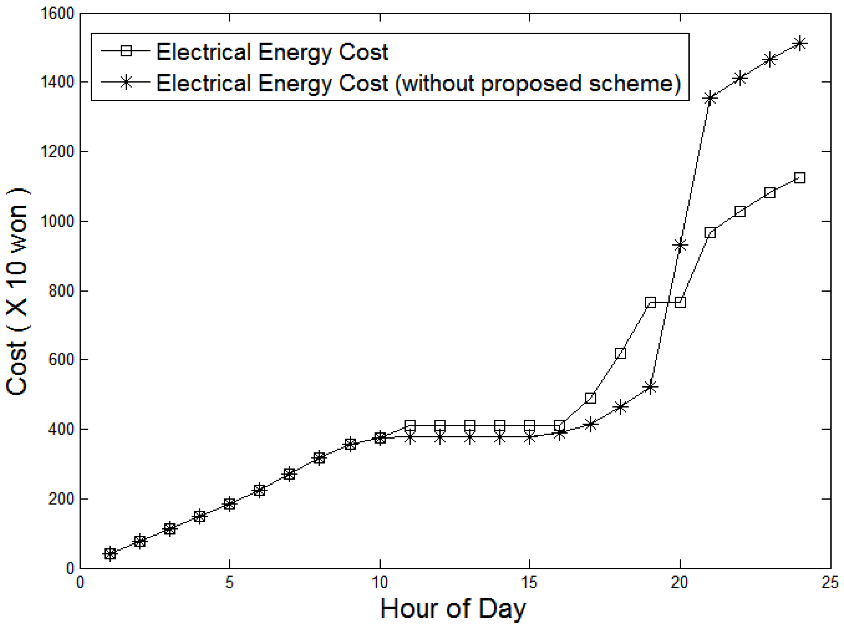
5.3. Scenario 2
Scenario 2 adopts the same loading conditions as Scenario 1 (See
Figure 13), except that the solar irradiance is zero because of unfriendly weather condition, decreasing the PV power. When there is no PV power available, the proposed system uses battery and grid power as illustrated in
Figure 15, which also indicates that the system begins charging the battery based on the power shortage forecast during the peak period at the point of three hours prior to the peak time previously defined as the reference time. Consequently, the electricity cost under this scenario is greater than that in Scenario 1. Nevertheless,
Figure 16 shows that our system brings considerable cost savings by efficiently charging the battery in the absence of PV power.
Figure 15.
Use of PV power, SOC of the battery and electricity cost under Scenario 2.
Figure 15.
Use of PV power, SOC of the battery and electricity cost under Scenario 2.
Figure 16.
Comparison of electricity costs in Scenario 2.
Figure 16.
Comparison of electricity costs in Scenario 2.
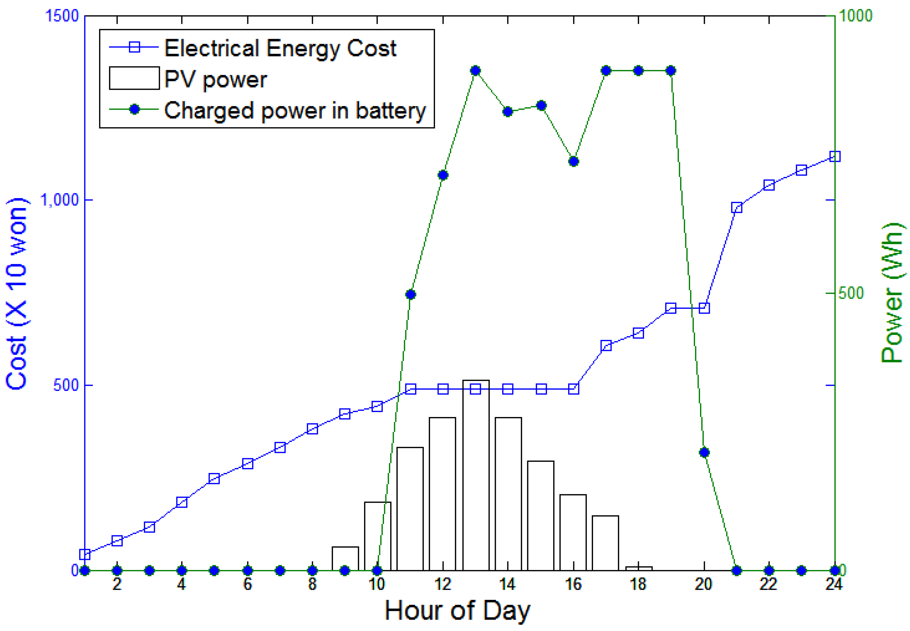
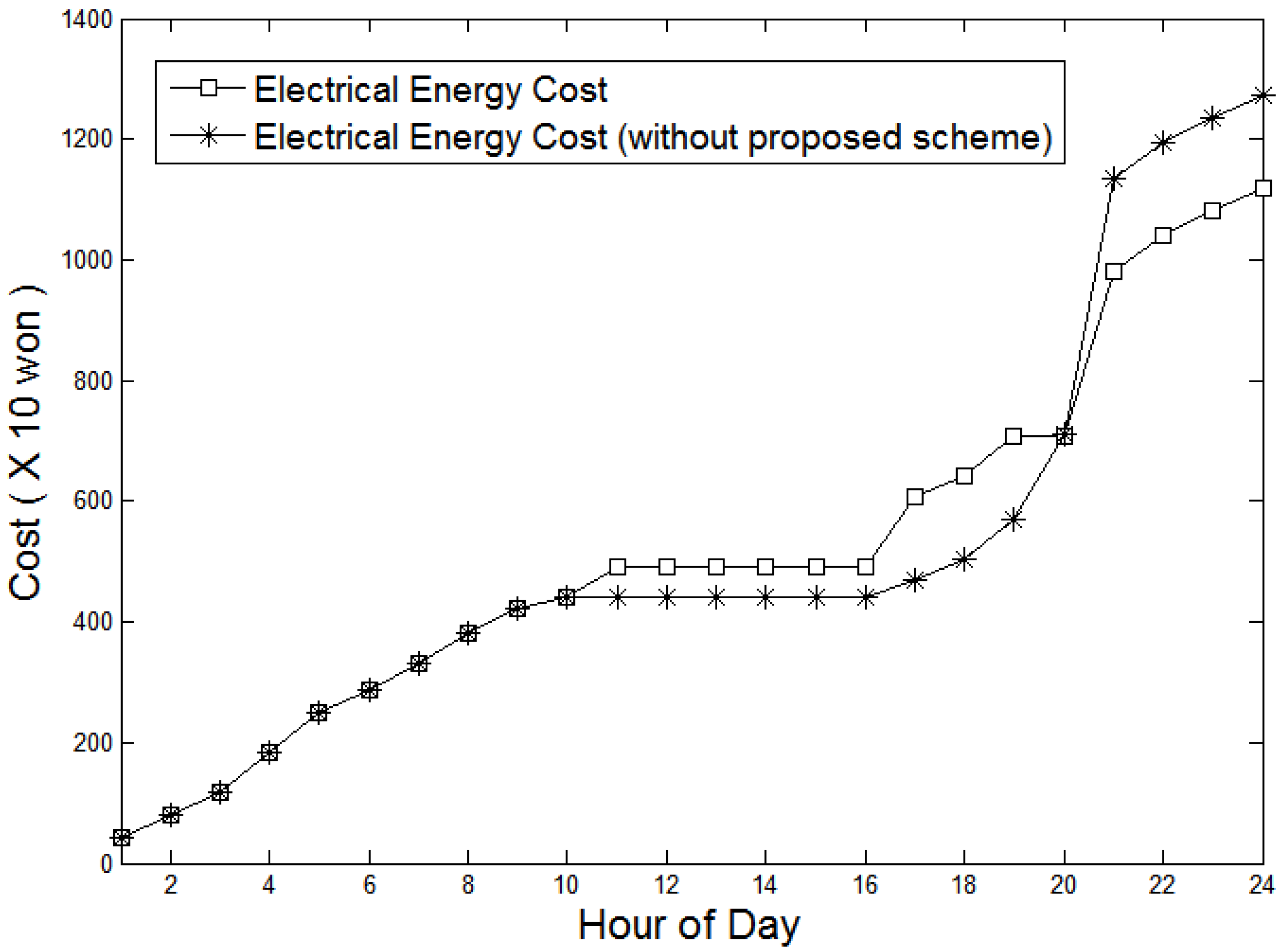
5.4. Scenario 3
Scenario 3 may be the worst condition, including serious load forecast error on top of the conditions of Scenario 2 as illustrated in
Figure 17. The power output from the PV, the charged power in the battery and the electricity cost are shown in
Figure 18. The battery is fully charged by 13:00 because there has been excess power available between 11:00 and 13:00, and the power output from the fully charged battery helps to reduce the electricity cost during the subsequent peak period. It is apparent in
Figure 19 that, even in this worst case, the proposed system operates stably and helps reduce cost.
Figure 17.
Actual and estimated load demands for Scenario 3.
Figure 17.
Actual and estimated load demands for Scenario 3.
Figure 18.
Use of PV power, battery charge status and electrical cost under Scenario 3.
Figure 18.
Use of PV power, battery charge status and electrical cost under Scenario 3.
Figure 19.
Comparison of electrical costs in Scenario 3.
Figure 19.
Comparison of electrical costs in Scenario 3.
6. Conclusions
This paper has investigated a practical grid-connected residential system consisting of a PV, a battery and grid power under critical peak pricing. The PV generates power as the primary energy source, and the battery stores excess PV power and provides the charged power as needed. The system is grid-connected to ensure the reliability of power delivery. An effective premise power management scheme including load-forecasting based on the Kalman filter has also been developed. The load-forecasting model accurately forecasts the next day’s load demand. Using the forecasting model in conjunction with the management scheme, the proposed system controls the system components and economizes the use of electricity by taking the CPP of grid power into account. We performed studies for three different scenarios using actual load demand, weather and household size data in order to verify the performance of the proposed system. The results demonstrate that the proposed system yields cost savings while providing reliable electricity service in a CPP market.


 ,
, 
