Finding Multiple Optimal Solutions to Optimal Load Distribution Problem in Hydropower Plant

Abstract

Optimal load distribution (OLD) among generator units of a hydropower plant is a vital task for hydropower generation scheduling and management. Traditional optimization methods for solving this problem focus on finding a single optimal solution. However, many practical constraints on hydropower plant operation are very difficult, if not impossible, to be modeled, and the optimal solution found by those models might be of limited practical uses. This motivates us to find multiple optimal solutions to the OLD problem, which can provide more flexible choices for decision-making. Based on a special dynamic programming model, we use a modified shortest path algorithm to produce multiple solutions to the problem. It is shown that multiple optimal solutions exist for the case study of China’s Geheyan hydropower plant, and they are valuable for assessing the stability of generator units, showing the potential of reducing occurrence times of units across vibration areas.

1. Introduction

Worldwide, hydropower plants produce about one-quarter of the world’s electricity and supply more than 1 billion people with electric power [1]. For example, there are more than 11,000 hydropower plants operating in China, providing about 20% of the country total electric power and making hydropower the country’s largest renewable energy source [2]. It has been shown that improving the operation of hydropower plants can increase the total profit by 1%–3% [3], which is of great significance for making energy production more efficient and reducing greenhouse gas emissions.

Hydropower plant operation involves issues such as optimal load distribution (OLD) and unit commitment [4,5]. In this paper, the OLD problem is defined as a deterministic optimization problem with a fixed hydraulic head and a single time step [6], namely economic dispatch. The objective is to minimize the total water discharge by optimizing the load distribution among multiple generator units. Since the OLD is a subproblem involved in unit commitment problems, it is a basic and vital module for a hydropower plant’s economic operation and generation scheduling [4].

It is noted that the OLD problem does not take into account the following factors: the amount of water in the basin is limited and therefore the objective usually aims at finding the optimal production levels at each period of an optimization horizon (e.g., a week) in order to achieve the maximum benefits from the limited quantity of water available in the basin; the level of the water in the basin (i.e., the hydraulic head) influences also the amount of electric energy that could be produced by a given amount of water.

A wide range of optimization methods have been applied to solving the OLD problem, including mixed integer linear programming (MILP) [7,8,9,10,11,12], mixed integer nonlinear programming [13], dynamic programming (DP) [14,15,16], Lagrangian relaxation [12,17,18], hierarchical optimization [6,19,20,21,22,23], genetic algorithm (GA) [18], particle swarm optimization (PSO) [2,24,25,26,27] and cultural algorithm [28]. These methods generally produce a single optimal or near-optimal solution. However, to practically assist the operation of large-scale hydropower plants, it is often more useful to provide a set of alternatives to decision makers so that they can choose the most appropriate solution. This is especially important because some practical constraints, such as the stability of generator units, are difficult to be taken into account in the optimization models.

There are many situations in which multiple optimal solutions (MOS) (i.e., solutions with the same objective value but with different values for the decision variables) may exist. For example, a general non-convex function, such as $sin\left(x\right)$, has multiple minima and maxima. For the OLD problem, the input/output (I/O) function of a generator is often non-convex, piece-wise linear with many pieces having the same slopes (Figure 1) [8]. In this case, suppose $x_1^{*},x_2^{*}$ are the optimal loads for generators 1 and 2, and suppose $x_1^{*}$ and $x_2^{*}$ on the pieces with the same slopes, then we can freely adjust $x_1^{*}$ and $x_2^{*}$ by the same amounts but in the opposite direction while still achieving the same objective value and satisfying the fixed total load constraint. In fact, it was reported that there were MOS for the refill operation of the Three Gorges Reservoir in China [29].

Figure 1. An example showing that multiple solutions might exist in the OLD problem.

Figure 1. An example showing that multiple solutions might exist in the OLD problem.

MOS have been studied in different contexts. For example, in integer linear programming, all optimal solutions are found by iteratively solving the original problem with new integer constraints added to exclude the optimal solutions found from the previous iterations [30]. For general nonlinear programming problems, a dynamical trajectory-based methodology was developed for computing multiple local optimal solutions [31]. In the shortest path problem, all the optimal and near-optimal solutions are found by using a near-shortest path algorithm, which is a modified version of backtracking in DP [32]. For general optimization problems, the Niche PSO technique was developed to locate and refine MOS [33]. The multiple near-optimal solutions, whose objective values are equal or sufficiently close to the optimum, were explored in the deterministic reservoir operation problems [34]. However, as far as we know, the problem of finding multiple solutions has not been addressed in the OLD problem. In fact, we will show in the case study that MOS do exist in the OLD problem.

In the rest of this paper, we present the description for the OLD problem in Section 2, followed by our solution approach in Section 3. Using discretization, which is usually used to solve DP models, we reformulate the discretized OLD problem as a shortest path problem. We then develop a special shortest path algorithm to find MOS. The case study of the Geheyan hydropower plant is then shown in Section 4. Section 5 draws the conclusions of this research.

Since the discretization resolution affects the optimality of the solutions found, our method requires a reference or benchmark on the optimum as a guidance for the discretization. Therefore, though the focus of this study is on finding multiple solutions, we also provide models for finding an optimal solution in the Appendix as well. These include a MILP model to find the global optimal solution for the case of piece-wise linear I/O function and a Lagrangian relaxation model for general I/O functions. Additionally, we provides some cases with a nonlinear I/O function to illustrate that MOS might also exist in the OLD problem.

2. Problem Description

The problem of optimal load distribution among hydropower plant units is to minimize the total water discharge while ensuring the power system reliability [2,4,6]. This problem is modeled as follows:

$$\begin{array}{c}\hfill \begin{array}{cc}\hfill Q^{*}& =min\sum _{i=1}^n{Q}_i\left(x_i\right)\hfill \\ \hfill s.t.\sum _{i=1}^n{x}_i& =L,x_i\in R_i,\forall i=1,\dots ,n\hfill \end{array}\end{array}$$

(1)

where n is the number of generator units, $x_i$ and $Q_i\left(x_i\right)$ are the electric load and the water discharge for generator unit i respectively. L is the required total electric load for the hydropower plant. $R_i$ is the feasible load for generator unit i and is often equivalent to $[l_i,z_i^l]\cup [z_i^u,u_i]$, i.e., either $l_i\le x_i\le z_i^l$ or $z_i^u\le x_i\le u_i$. The minimum $l_i$, maximum $u_i$ and infeasible range $(z_i^l,z_i^u)$ for unit i impose the operational constraints upon the real-time unit commitment and load distribution. The infeasible range $(z_i^l,z_i^u)$ is defined as the vibration area where the generator shaft tends to vibrate violently [35]. It should be noted that this problem is independent of time.

The water discharge function $Q_i\left(x_i\right)$ is often non-convex and hence the OLD problem shown in (1) often has a non-convex objective function [36]. In addition, the feasibility space is discontinuous due to the vibration range of the loads. Therefore, the OLD problem is often very difficult to solve even for finding just a single optimal solution. In fact, traditional methods such as Lagrangian relaxation, MILP or DP often can only find a near-optimal solution. On the contrary, our method will find multiple optimal or near-optimal solutions using discretization and a shortest path algorithm.

3. Solution Approach for Finding Multiple Solutions

We notice that the OLD problem has only one join constraint on the decision variables, i.e., ${\displaystyle \sum _{i=1}^n}{x}_i=L$. This special structure allows us to consider applying dynamic programming algorithms. We first review the general DP framework in Subsection 3.1 to show the general idea. However, this general framework and traditional DP algorithms might not work for the OLD problem due to the non-convexity of the objective function and a discontinuous feasible region. This leads to the idea of using discretization that allows us to find not only a single optimal solution but a multiple of them.

3.1. Review of General Dynamic Programming (DP) Framework

DP, based on Bellman’s principle, is a classic optimization method that improves computational efficiency greatly by saving some intermediate results into memory, which can be reused [37]. A DP model can be formulated by the following procedures [14,15]:

(1)

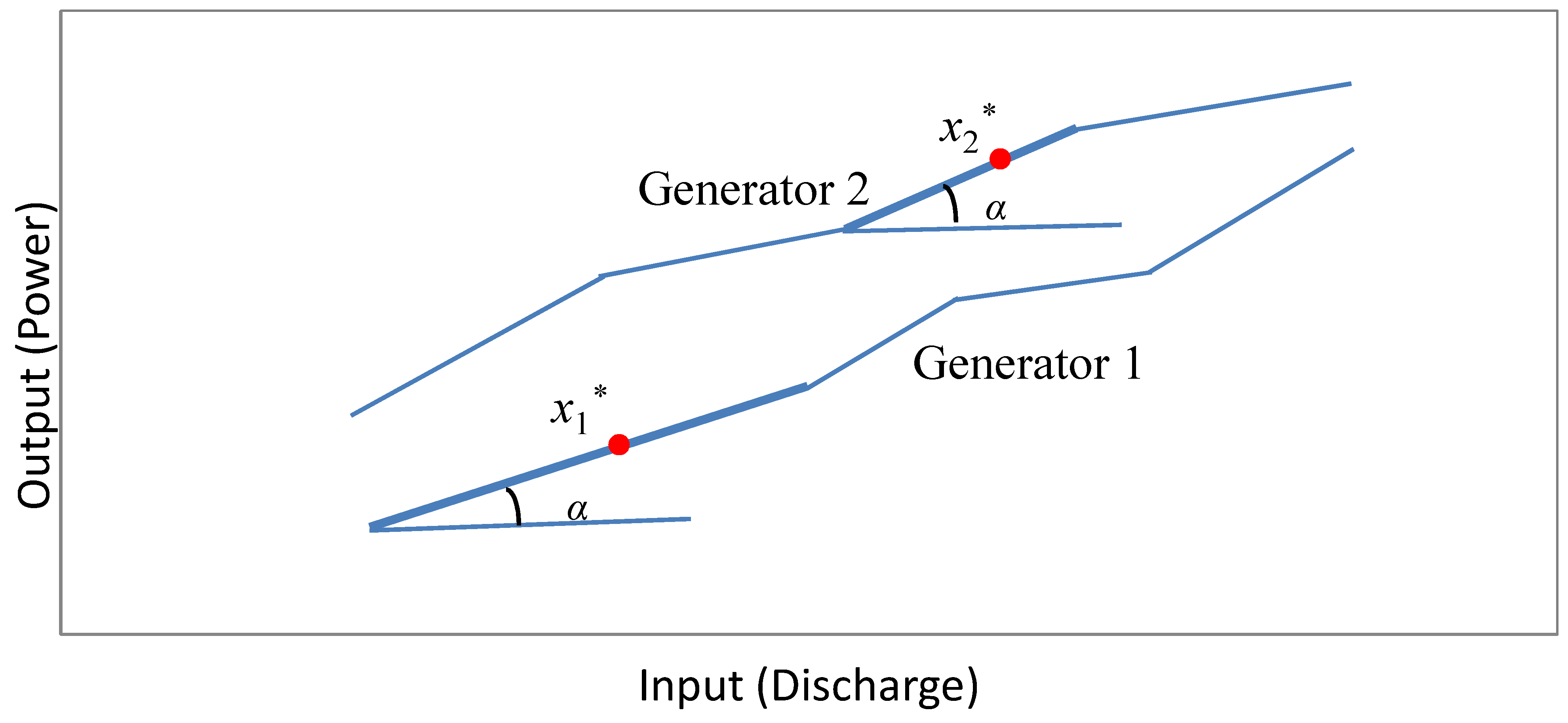
Setting the decision variable $x_i$ as the load allocated to the $i^{th}$ generator.

(2)

Setting the stage variable as the accumulative load of the first i generators: $s_i={\displaystyle \sum _{j=1}^i}{x}_i$.

(3)

Establishing the state equation as:

$$\begin{array}{c}\hfill s_i=s_{i-1}+x_i\end{array}$$

(2)

(4)

Define $f_i\left(s_i\right)$ as the minimum total water discharge when the accumulative electric load from the first generator to the $i^{th}$ one is $s_i$, i.e.,

$$\begin{array}{c}\hfill \begin{array}{cc}\hfill f_i\left(s_i\right)& =\underset{x_1,x_2,\dots ,x_i}{min}\sum _{j=1}^i{Q}_j\left(x_j\right)\hfill \\ \hfill s.t.\sum _{j=1}^i{x}_j& =s_i,x_j\in R_j,\forall j\in \{1,\dots ,i\}\hfill \end{array}\end{array}$$

(3)

We also defined $f_i\left(s_i\right)=\infty$ if equation (3) is infeasible. Then problem (1) is equivalent to finding $f_n\left(L\right)$. We can find $f_i\left(s_i\right)$ recursively using the following Bellman equation:

$$\begin{array}{c}\hfill f_i\left(s_i\right)=\underset{x_i\in R_i}{min}\{Q_i\left(x_i\right)+f_{i-1}(s_i-x_i)\}\end{array}$$

(4)

where $f_0\left(s_0\right)=0$ is defined as the boundary condition.

In the cases when the I/O function is quadratic and there is no constraint on the loads, we can find the closed form for $f_i\left(s_i\right)$ and the optimal load distribution $x_i$. However, this is not the case for the OLD problem since the discharge function is non-convex and the feasible range is discontinuous. We can also try approximate dynamic programming [38] to approximate $f_i\left(s_i\right)$. However, this method might be time consuming and inaccurate because of the discontinuous feasible region involves in this problem.

We will discretize the feasible space of the loads and show that the discretized OLD problem is equivalent to a shortest path problem that can be solved efficiently. The discretization resolution is adjusted such that the optimum total discharge found by the discretized OLD is relatively close to the optimum total discharge found using Lagrangian relaxation or MILP methods (see Appendix A). We modify the shortest path algorithm slightly to keep track of all the optimal paths. Although discretization generally provides only approximate solutions, near-optimal solutions are often accepted in practice. In addition, for this particular case study, we will show that the solutions obtained were actually the global optima solutions.

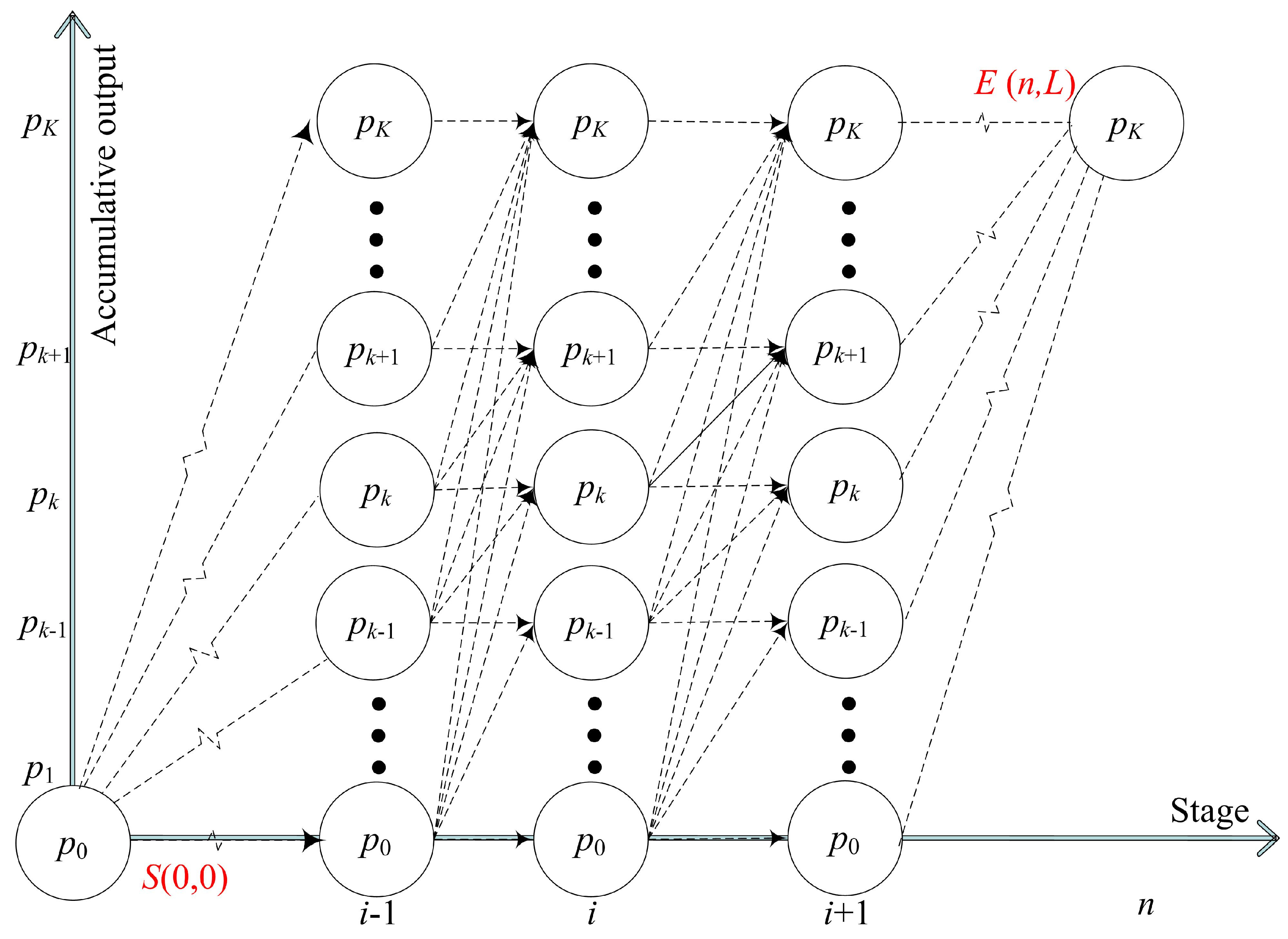
3.2. Discretized OLD as a Shortest Path Problem

The decision variable $x_i$ in the OLD problem is continuous and can take any value in its feasible domain $R_i$. Let us discretize the interval $[0,L]$ into discrete values $\{p_0,p_1,\dots ,p_K\}$ with $p_j=j\Delta$, $\forall j=0,1,\dots ,K$ and $\Delta =L/K$. Suppose we can impose a further constraint that $x_i\in \{p_0,p_1,\dots ,p_K\}$, and consider a new optimization problem:

$$\begin{array}{c}\hfill \begin{array}{cc}\hfill min& \sum _{i=1}^n{Q}_i\left(x_i\right)\hfill \\ \hfill s.t.& \sum _{i=1}^n{x}_i=L,x_i\in S_i,\forall i=1,\dots ,n\hfill \end{array}\end{array}$$

(5)

where $S_i$ is defined to be the feasible set for $x_i$ in the discretized OLD problem, i.e.,

$$S_i=\left\{x_i|x_i\in R_i,x_i\in \{p_0,p_1,\dots ,p_K\}\right\}$$

It is noted that an optimal solution of the new problem shown in Equation (5) might be different from that of the original (continuous) problem shown in Equation (1). In addition, the optimum of the new problem should not be smaller than that of the original problem. However, if the discretization resolution is fine enough and if multiple solutions do exist, the gap could be small. In fact, we will show in the case study that the discretized problem can produce optimal solutions.

We will show how the discretized OLD problem can be reformulated as a shortest path problem. In the two dimensional coordinate system, we draw coordinates $(i,p_k)$ where $i=\{0,1,\dots ,n\}$ and $k=\{0,1,\dots ,K\}$. Let $(x_1,x_2,\dots ,x_n)$ be a feasible solution to the discretized OLD problem, i.e., ${\sum }_{i=1}^n{x}_i=L$ and $x_i\in S_i$. In Figure 2, we draw the points $(0,0)$, $(1,s_1)$, $(2,s_2),\dots ,(n,s_n)$ on the two dimensional coordination system, where $s_i={\sum }_{j=1}^i{x}_i$. If we connect the points sequentially, we obtain a path from $(0,0)$ to $(n,L)$. In other words, each of the paths from $(0,0)$ to $(n,L)$ would be a solution to the total load constraint ${\sum }_{i=1}^n{x}_i\equiv L$. We also set the cost of the arc from coordinate $(i-1,s_{i-1})$ to coordinate $(i,s_i)$ is set as follows:

$$\begin{array}{c}\hfill c_{(i-1,s_{i-1})\to (i,s_i)}=\left\{\begin{array}{cc}{Q}_i\left(x_i\right),\hfill & \text{if}{x}_i\in S_i\hfill \\ \infty \hfill & \text{otherwise}.\hfill \end{array}\right.\end{array}$$

(6)

Then, the total cost of the path would be the total discharge ${\sum }_{i=1}^n{Q}_i\left(x_i\right)$ when $(x_1,x_2,\dots ,x_n)$ is a feasible solution. The discretized OLD problem is equivalent to finding a shortest path from the origin $(0,0)$ to the destination $(n,L)$. We then can apply different shortest path algorithms to solve the discretized OLD problem efficiently [39].

Figure 2. A solution to the discretized OLD problem can be viewed as path from the origin $S(0,0)$ to the destination $E(n,L)$.

Figure 2. A solution to the discretized OLD problem can be viewed as path from the origin $S(0,0)$ to the destination $E(n,L)$.

Figure 3 shows that the discretized OLD problem becomes the shortest path problem from the origin $(0,0)$ to $(n,L)$. The nodes of the network represent the accumulative loads, the edges represent the load distribution and the costs of the edges are the water discharges.

Figure 3. The discretized OLD is equivalent to a shortest path problem for finding an optimal path from the origin $(0,0)$ to the point $(n,L)$ that passes through the points on the grid.

Figure 3. The discretized OLD is equivalent to a shortest path problem for finding an optimal path from the origin $(0,0)$ to the point $(n,L)$ that passes through the points on the grid.

3.3. Finding MOS

The solution approach for finding MOS in the OLD problem is same as the standard shortest path algorithm. Let us define $q(i,p_k)$ as follows:

$$\begin{array}{c}\hfill \begin{array}{cc}\hfill q(i,p_k)& =\underset{x_1,x_2,\dots ,x_i}{min}\sum _{j=1}^i{Q}_j\left(x_j\right)\hfill \\ \hfill s.t.\sum _{j=1}^i{x}_j& =p_k,x_j\in S_j,\forall j\in \{1,\dots ,i\}\hfill \end{array}\end{array}$$

(7)

which is a discretized version of $f_i\left(p_k\right)$ as shown in the general DP framework in Equation (4). We define $q(i,p_k)=\infty$ if the problem is infeasible.

The idea of a shortest path algorithm is to solve the subproblems with small i and k and then use the results to solve subproblems with larger $i,k$ until $i=n$ and $p_k=L$. In addition, this algorithm keeps track of all the optimal subpaths to produce multiple solutions for the shortest paths.

We have:

$$\begin{array}{c}\hfill q(i,p_k)=\underset{x_i\in S_i}{min}\{q(i-1,p_k-x_i)+Q_i\left(x_i\right)\}\end{array}$$

(8)

This is basically the Bellman equation or the principle of optimality [37]. This equation is equivalent to saying that the optimal path from the origin $(0,0)$ to $(i,p_k)$ can be found by identifying the points among the set of $(i-1,p_k-x_i)$, i.e., the best points with the minimum total cost as shown in Figure 3. The following shortest path algorithm shows the formal procedure for finding an OLD solution:

• For $i=1$:
  We set $q(1,p_k)$ for $k\in \{1,2,\dots ,K\}$ as follows:

  $$\begin{array}{c}\hfill q(1,p_k)=\left\{\begin{array}{cc}{Q}_1\left(p_k\right)\hfill & \text{if}{p}_k\in S_1\hfill \\ \infty \hfill & \text{otherwise}\hfill \end{array}\right.\end{array}$$

  (9)
• For $i=2$ to n:
  We set $q(i,p_k)$ for $k=\{1,2,\dots ,K\}$ as follows:

  $$\begin{array}{c}\hfill q(i,p_k)=\underset{x_k\in S_k}{min}\left\{q(k-1,p_j-x_k)+Q_k\left(x_k\right)\right\}\end{array}$$

The number of operations for each i that is in the range $[2,n-1]$ is, at most, the number of links between node $(i,k)$ and $(i+1,k^{\prime })$, which is equal to $\frac{K(K+1)}{2}$. The number of operations for $i=1$ and $i=n$ are at most K each. Thus, the total number of evaluations is at most $(n-2)K^2+2K$.

To find of all the optimal solutions, we can modify the traditional shortest path algorithm slightly to keep track of the optimal subpaths. The idea is to use the principle of optimality in dynamic programming as follows: if an optimal path from $(0,0)$ to $(i,p_k)$ contains the point $(i-1,p_{k^{\prime }})$, then the set of all the optimal subpaths to $(i-1,p_{k^{\prime }})$ is also contained in the set of all the optimal subpaths to $(i,p_k)$.

Let $D(i,p_k)$ be the set of all the optimal solutions of problem (7) at each $i\ge 1$ and $p_k$ (each optimal solution is a vector of length i). Let $\{x_{i1}^{*},\dots ,x_{im}^{*}\}$ be the set of optimal solutions for the recursive problem (8). Then, with $i=1$, we have:

$$\begin{array}{c}\hfill D_{1,j}=\left\{\begin{array}{cc}{p}_j\hfill & \text{if}{p}_j\in S_1\hfill \\ \varnothing \hfill & \text{otherwise}\hfill \end{array}\right.\end{array}$$

and with $i\ge 2$, we have:

$$\begin{array}{c}\hfill D(i,p_k)=\left\{(D(i-1,p_k-x_{i1}^{*}),x_{i1}^{*}),\dots ,(D(i-1,p_k-x_{im}^{*}),x_{im}^{*})\right\}\end{array}$$

The formal modified shortest path algorithm for finding MOS of the OLD is as follows:

• For $i=1$:
  We set $q(1,k)$ for $k\in \{1,2,\dots ,K\}$ as follows:

  $$\begin{array}{cc}\hfill q(1,k)& =\left\{\begin{array}{cc}{Q}_1\left(p_k\right)\hfill & \text{if}{p}_k\in S_1\hfill \\ \infty \hfill & \text{otherwise}\hfill \end{array}\right.\hfill \end{array}$$

  and

  $$\begin{array}{cc}\hfill D(1,p_k)& =\left\{\begin{array}{cc}{p}_k\hfill & \text{if}{p}_k\in S_1\hfill \\ \varnothing \hfill & \text{otherwise}\hfill \end{array}\right.\hfill \end{array}$$
• For $i=2$ to n:
  We set $q(i,p_k)$ for $k=\{1,2,\dots ,K\}$ as follows:

  $$\begin{array}{c}\hfill {\displaystyle q(i,p_k)=\underset{x_i\in S_i}{min}\left\{q(i-1,p_k-x_i)+Q_i\left(x_i\right)\right\}}\end{array}$$

  If $q(i,p_k)<\infty$, we set,

  $$\begin{array}{c}\hfill D(i,p_k)=\left\{(D(i-1,p_k-x_{i1}^{*}),x_{i1}^{*}),\dots ,(D(i-1,p_k-x_{im}^{*}),x_{im}^{*})\right\}\end{array}$$

  where $\{x_{i1}^{*},\dots ,x_{im}^{*}\}$ are the optimal solutions of problem (8). Otherwise, we set $D(i,p_k)=\varnothing$.

Notice that the algorithm works with all types of I/O functions and the discontinuous feasible region involved in this problem.

The algorithm’s computational complexity includes two parts: (1) the traditional computational complexity for the shortest path, which is $(n-2)K^2+2K$; and (2) the computational complexity for procedure of trace back, M, which is the number of multiple optimal solutions. Since the M is not often a large number, the proposed approach could offer a practical solution in terms of computation time.

3.4. Multiple Solutions Space

The multiple solutions found by the special shortest path algorithm are scattered points in space. However, the space of all the optimal solutions could form continuous regions. In the case of piece-wise linear discharge functions, we can find this space by using marginal utility analysis. Among all the optimal solutions for which the constraints $x_i\in R_i$ are not binding, the marginal utilities must be the same, i.e., $\frac{\partial Q_1}{\partial x_1}=\frac{\partial Q_2}{\partial x_2}=\cdots =\frac{\partial Q_n}{\partial x_n}$. Let $x_{i1}^{*},x_{i2}^{*},\dots ,x_{im}^{*}$ be a particular set of optimal unit loads. Then we can perturb these solutions at the same time such that their sum does not change. For example, we can adjust the optimal solution to $x_{i1}^{*}+ϵ,x_{i2}^{*}-ϵ$, where ϵ is small enough, while keeping all other unit loads unchanged. The range of ϵ is chosen so that the new loads $x_{i1}^{*}+ϵ$ and $x_{i2}^{*}-ϵ$ still lie within their original linear pieces of the piece-wise discharge functions.

4. Case Study

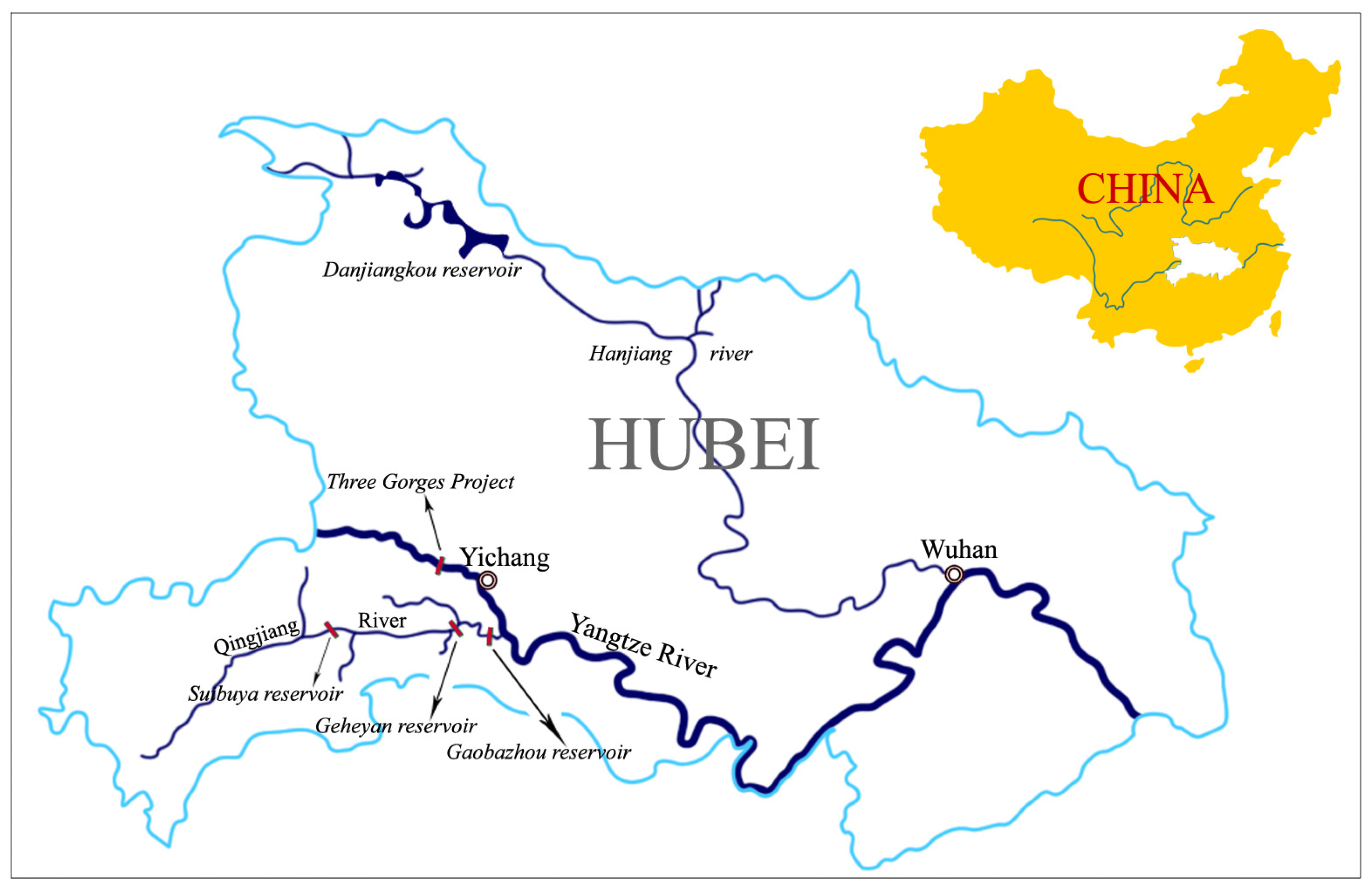
4.1. Geheyan Hydropower Plant

As shown in Figure 4, the Geheyan hydropower plant is located about 9 km upstream of the Qing River from Changyang county, Hubei Province in China. The plant has a large hydropower generation capacity of $2.94\times {10}^9$ kWh per year with a firm output of $2.41\times {10}^5$ kW. The area of the Geheyan reservoir basin is 14,430 km${}^2$. Corresponding to normal and minimum water levels of 200 m and 160 m, respectively, the normal and dead water storage are $3.12\times {10}^9$ m ${}^3$ and $1.98\times {10}^9$ m${}^3$. The reservoir is used for inter-year flow regulation.

Figure 4. Map showing the location of the Geheyan Hydropower plant in China.

Figure 4. Map showing the location of the Geheyan Hydropower plant in China.

The plant is equipped with four generation units, which have the same I/O curves. It should be noted that the same I/O curves are only an approximate for practice, which was provided by the generator factory. For a single generation unit, some records of the I/O curve for a water head of 110 m are plotted in Figure 5. The minimum output is 10 MW and the vibration area ranges from 80 MW to 180 MW. The model is described as follows:

$$\begin{array}{c}\hfill \begin{array}{cc}\hfill min{Q}^{*}& =\sum _{i=1}^4{Q}_i\left(x_i\right)\hfill \\ \hfill s.t.\sum _{i=1}^4{x}_i& =L,\hfill & \hfill x_i& \notin [80,180]\hfill \\ & & \hfill x_i& \ge 10\forall i=1,\dots ,n\hfill \\ & & \hfill x_i& \le 300\hfill \end{array}\end{array}$$

(10)

Figure 5. Efficiencies of generator in the Geheyan Hydropower plant for 110 m water head.

Figure 5. Efficiencies of generator in the Geheyan Hydropower plant for 110 m water head.

Based on these records, a piece-wise linear approximating technique is used to describe the I/O curve. It very often uses this piece-wise linear I/O function in practical operation of hydropower plants [5].

4.2. Global Optimal Solution

The MILP model (Appendix B) is used to find the optimal solution (reference or benchmark), in which the I/O curve of generation unit is a piece-wise linear function and a penalty function method (by modification of the I/O curve) is used to avoid vibration. Lingo 9.0^® [40] is used to solve the MILP model. The global optimal solutions are listed in Table 1 when the total electric load varies from 500 MW to 1200 MW. For simplicity, an assumption is made that the outputs of these units decline from unit 1 to unit 4.

Table 1. The results of global optimal solution to the OLD problem by using MILP.

Load L (MW)	Output of units (MW)				Total discharge $Q^{*}$ (m${}^3$/s)	Total discharge $Q_L^{*}$ (m${}^3$/s)
	Unit 1 ${\mathit{x}}_{\mathbf{1}}^{*}$	Unit 2 ${\mathit{x}}_{\mathbf{2}}^{*}$	Unit 3 ${\mathit{x}}_{\mathbf{3}}^{*}$	Unit 4 ${\mathit{x}}_{\mathbf{4}}^{*}$
500	255	245	\	\	518	517.1
550	295	255	\	\	562	562.0
600	300	300	\	\	608	608.0
650	295	285	70	\	688	686.3
700	265	255	180	\	734	731.0
750	250	250	250	\	777	775.6
800	295	255	250	\	821	820.5
850	300	295	255	\	866	865.5
900	300	300	300	\	912	912.0
950	295	295	295	65	991	989.5
1,000	255	255	255	235	1,036	1,034.2
1,050	275	265	255	255	1,079	1,079.0
1,100	275	275	275	275	1,124	1,124.0
1,150	295	295	295	265	1,169	1,169.0
1,200	300	300	300	300	1,216	1,216.0

Table 1. The results of global optimal solution to the OLD problem by using MILP.

Load L (MW)	Output of units (MW)				Total discharge $Q^{*}$ (m${}^3$/s)	Total discharge $Q_L^{*}$ (m${}^3$/s)
	Unit 1 ${\mathit{x}}_{\mathbf{1}}^{*}$	Unit 2 ${\mathit{x}}_{\mathbf{2}}^{*}$	Unit 3 ${\mathit{x}}_{\mathbf{3}}^{*}$	Unit 4 ${\mathit{x}}_{\mathbf{4}}^{*}$
500	255	245	\	\	518	517.1
550	295	255	\	\	562	562.0
600	300	300	\	\	608	608.0
650	295	285	70	\	688	686.3
700	265	255	180	\	734	731.0
750	250	250	250	\	777	775.6
800	295	255	250	\	821	820.5
850	300	295	255	\	866	865.5
900	300	300	300	\	912	912.0
950	295	295	295	65	991	989.5
1,000	255	255	255	235	1,036	1,034.2
1,050	275	265	255	255	1,079	1,079.0
1,100	275	275	275	275	1,124	1,124.0
1,150	295	295	295	265	1,169	1,169.0
1,200	300	300	300	300	1,216	1,216.0

The Lagrangian relaxation method (Appendix A) is also applied to find lower bounds of the optimal total water discharges. This method is often applicable in cases when the problem size is large (i.e., with large n and with more complex I/O function). The total water discharge, $Q_L^{*}$, are shown in Table 1. For example, a lower bound total water discharge of 517.1 m${}^3$/s is found when the load is set to 500 MW, which is quite close to the true optimum of 518 m${}^3$/s. We can also see that in some cases, e.g., with $L=\{550,600,900\}$, the optimal objective value of the OLD problem is equal to one obtained using the Lagrangian relaxation method. Nevertheless, both the MILP model and the Lagrangian relaxation method produce only a single solution. The focus of our paper is on finding MOS as we will show in the next subsection.

4.3. Multiple Solutions

The multiple-solution approach is implemented to find all solutions to the OLD problem of the Geheyan hydropower plant. The computation time is several seconds for a specific load. More than one solution is obtained, all of which have the same total water discharge as that of MILP. Some typical cases are described as follows.

(1)

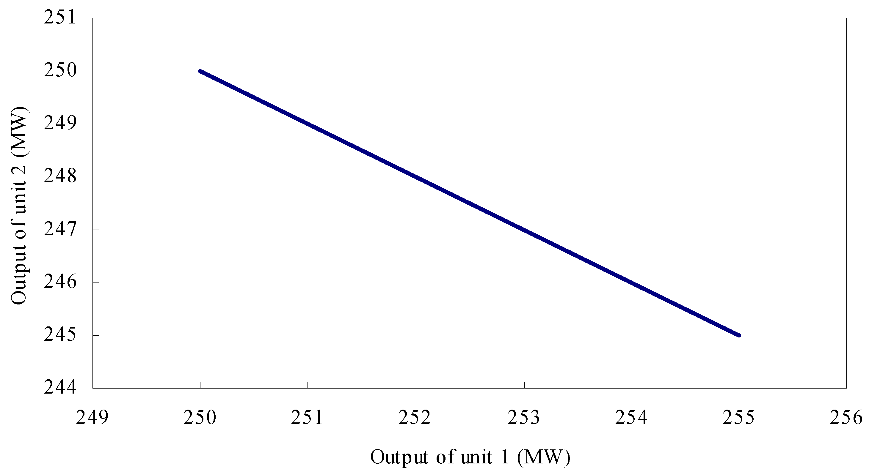
In the case that total electric load is equal to 500 MW ($L=500$), the optimal solution consumes water discharge of 518 m${}^3$/s and distributes them to unit 1 and unit 2 (Table 1).

Table 2 shows single or multiple solutions under different discrete intervals. When the discrete interval of DP is 100 MW, a single solution is found but it is not optimal compared to the optimal water discharge found from MILP (518 m${}^3$/s). When the discrete interval is 10 MW, a single optimal solution is located. When the discrete interval decreases to 1 MW, multiple solutions are found and they all reach the optimal discharge. With a smaller interval (0.1 MW), even more optimal solutions are identified.

Table 2. The relationship between discrete the interval and solutions in load of 500 MW.

Discrete interval	Unit 1	Unit 2	Total discharge
Δ (MW)	${\mathit{x}}_{\mathbf{1}}^{*}$ (MW)	${\mathit{x}}_{\mathbf{2}}^{*}$ (MW)	${\mathbf{Q}}^{*}$ (m${}^{\mathbf{3}}$/s)
100	300	200	521
10	250	250	518
1	255	245	518
	254	246
	⋮	⋮
	251	249
	250	250
0.1	255	245	518
	254.9	245.1
	⋮	⋮
	250.1	249.9
	250	250

Table 2. The relationship between discrete the interval and solutions in load of 500 MW.

Discrete interval	Unit 1	Unit 2	Total discharge
Δ (MW)	${\mathit{x}}_{\mathbf{1}}^{*}$ (MW)	${\mathit{x}}_{\mathbf{2}}^{*}$ (MW)	${\mathbf{Q}}^{*}$ (m${}^{\mathbf{3}}$/s)
100	300	200	521
10	250	250	518
1	255	245	518
	254	246
	⋮	⋮
	251	249
	250	250
0.1	255	245	518
	254.9	245.1
	⋮	⋮
	250.1	249.9
	250	250

The multiple solutions space can be found by the marginal utility principle, $\frac{\partial Q_1}{\partial x_1}=\frac{\partial Q_2}{\partial x_2}=\cdots =\frac{\partial Q_n}{\partial x_n}$, e.g., $\frac{\partial Q_1}{\partial x_1}=\frac{263-259}{255-250}=\frac{\partial Q_2}{\partial x_2}=\frac{259-255}{250-245}$. Figure 6 shows the existence of MOS on a line segment.

Figure 6. Multiple solutions to total electric load of 500 MW (output of unit 1 ≥ output of unit 2).

Figure 6. Multiple solutions to total electric load of 500 MW (output of unit 1 ≥ output of unit 2).

(2)

When total load is set to 650 MW, four multiple solutions spaces are identified as follows.

(a)

$x_1^{*}\in [290,295]$, $x_2^{*}\in [290,295]$ and $x_3^{*}\in [60,65]$. These ranges, if satisfying OLD constraints, can be verified by the records of the I/O curve, e.g., $\frac{299-295}{295-290}=\frac{299-295}{295-290}=\frac{94-90}{65-60}$. Furthermore, we can obtain multiple solutions from $x_1^{*}=290+{ϵ}_1$, $x_2^{*}=290+{ϵ}_2$ and $x_3^{*}=70-{ϵ}_1-{ϵ}_2$ given any values of ${ϵ}_1$ and ${ϵ}_2$, $0\le {ϵ}_2\le {ϵ}_1\le 5$ and ${ϵ}_1+{ϵ}_2\ge 5$.

(b)

$x_1^{*}\in [295,300]$, $x_2^{*}\in [285,290]$ and $x_3^{*}\in [65,70]$.

(c)

$x_1^{*}\in [295,300]$, $x_2^{*}\in [295,300]$ and $x_3^{*}\in [55,60]$.

(d)

$x_1^{*}\in [295,300]$, $x_2^{*}\in [295,300]$ and $x_3^{*}\in [50,55]$.

These four areas of multiple solutions are shown in Figure 7 using a three-dimensional figure. This shows the existence of MOS in the form of a surface.

Figure 7. Multiple solutions space to total electric load of 650 MW (output of unit 1 ≥ output of unit 2 ≥ output of unit 3).

Figure 7. Multiple solutions space to total electric load of 650 MW (output of unit 1 ≥ output of unit 2 ≥ output of unit 3).

(3)

When the total load is set to 1100 MW, four generation units are used. By using the multiple solution approach, each unit’s output is either 295 MW, 285 MW, 275 MW, 265 MW or 255 MW. That is, if a solution sampled from above values satisfies the OLD constraints, it is an optimal solution. It is shown that the multiple solutions exist in the form of a few scattered points.

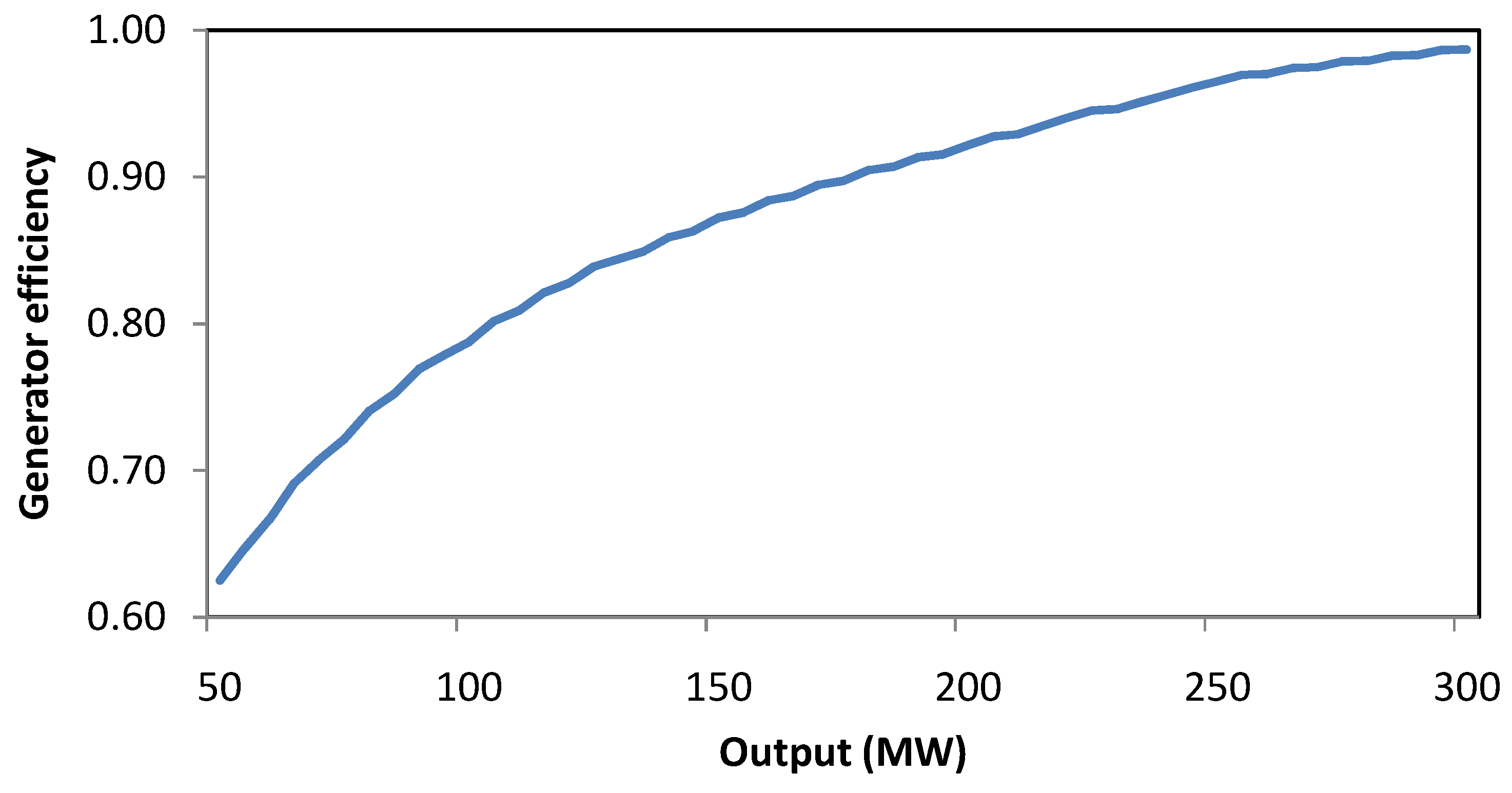
4.4. Non-Linear I/O Function

A second degree polynomial interpolation technique is used as a nonlinear approximation to the I/O curve. That is, the top three nearest points to $(P_{i,k-1},Q_{i,k-1})$, $(P_{i,k},Q_{i,k})$ and $(P_{i,k+1},Q_{i,k+1})$ are used to construct a quadratic function. This quadratic function is used to estimate the $Q_i\left(x_i\right)$. Based on the above approximation for the I/O curve, some cases are shown as follows.

(1)

In the case that total electric load is equal to 500 MW, the optimal solution consumes water discharge of 518 m${}^3$/s and distributes them to unit 1 and unit 2. Indeed, the multiple optimal solutions are the same as that from the piece-wise linear approximation (Figure 6) because the nonlinear and linear approximation are the same within the range of [240 MW, 255 MW].

(2)

In the case that total electric load is equal to 650 MW, (296.7 MW, 286.7 MW, 66.6 MW) is the unique optimal solution.

(3)

In the case that total electric load is equal to 1100 MW, a few scattered points, the same as that of piece-wise linear I/O curve, are the multiple optimal solutions.

The modified DP algorithm is also used in an economic dispatch problem, EXAMPLE 3D in [4] (See Appendix C), to illustrate that the multiple solutions can also exist for a theme plant with nonlinear I/O functions. When a discrete step of 0.1 MW is used for the computation (programming with a 32-bit floating-point data), some multiple optimal solutions have been found, such as (725.8 MW, 909.4 MW, 864.8 MW), (725.9 MW, 909.3 MW, 864.8 MW), (726.0 MW, 909.6 MW, 864.4 MW), (726.1 MW, 909.5 MW, 864.4 MW), (726.2 MW, 909.5 MW, 864.3 MW), (726.3 MW, 909.4 MW, 864.3 MW) and (726.7 MW, 909.0 MW, 864.3 MW). It should be noted that these solutions are not the extract optimal but near-optimal solutions, because they depend on the data length of the computer.

4.5. Application

In the practical operation of a hydropower plant, the total load L often changes from time to time. In these cases, a small increment in load results in a new dispatch, which may end with the most economical values as determined by the model, but is not acceptable from an operational point of view [21]. Typically, some MOS require one or more generators to drop or raise their output dramatically. We often want to avoid adjusting, especially through the vibration area since this may greatly affect production safety. Therefore, multiple solutions from OLD are valuable, since they provide more alternative schemes from which decision maker can choose as shown in the following examples:

(1)

Improving unit stability: Multiple solutions provide choices to reduce the readjustment efforts when certain conditions change. For example, the total load L often changes from time to time as shown in Table 3, which lists historical data from a practical operation of the Geheyan hydropower plant. If the decision maker has only a single solution, the solutions with different values of L could be very different from each other and hence the readjustment cost is often high when the plant switches from one total load to another. However, if the decision maker has MOS for each different L, he/she can choose the solutions that require the least adjustment. For example, the decision maker could change only the load for unit 2 and keep the load of unit 3 constant when the total load L changes (because the solutions in the space [75 MW, 85 MW] have the same cost). This choice can improve the stability of the overall system.

Table 3. The load distribution of units in practical operation.

Date	Output of Units (MW)				Load (MW) $\mathbf{L}$
	Unit 1 ${\mathit{x}}_{\mathbf{1}}^{*}$	Unit 2 ${\mathit{x}}_{\mathbf{2}}^{*}$	Unit 3 ${\mathit{x}}_{\mathbf{3}}^{*}$	Unit 4 ${\mathit{x}}_{\mathbf{4}}^{*}$
2006-3-23 10:30	0	76.5	78.9	0	155.4
2006-3-23 10:31	0	80.9	78.9	0	159.8
2006-3-23 10:32	0	81.9	78.9	0	160.8
2006-3-23 10:33	0	80.9	78.9	0	159.8

Table 3. The load distribution of units in practical operation.

Date	Output of Units (MW)				Load (MW) $\mathbf{L}$
	Unit 1 ${\mathit{x}}_{\mathbf{1}}^{*}$	Unit 2 ${\mathit{x}}_{\mathbf{2}}^{*}$	Unit 3 ${\mathit{x}}_{\mathbf{3}}^{*}$	Unit 4 ${\mathit{x}}_{\mathbf{4}}^{*}$
2006-3-23 10:30	0	76.5	78.9	0	155.4
2006-3-23 10:31	0	80.9	78.9	0	159.8
2006-3-23 10:32	0	81.9	78.9	0	160.8
2006-3-23 10:33	0	80.9	78.9	0	159.8

(2)

Avoiding unit adjustment over the vibration area: For example, the current total load is $L=971$ MW and the I/O function is piece-wise linear. We can apply our algorithm to find multiple solutions for this case. The MOS include the following two solutions:

Solution 1: $x_1^{*}=255.4$ MW, $x_2^{*}=255.3$ MW, $x_3^{*}=255.3$ MW and $x_4^{*}=205.0$ MW.

Solution 2: $x_1^{*}=299.8$ MW, $x_2^{*}=295.8$ MW, $x_3^{*}=295.4$ MW and $x_4^{*}=80$ MW.

We notice that all units in solution 1 are greater than 180 MW while one of the units in solution 2 is less than 80 MW, where [80 MW, 180 MW] is the vibration zone. Depending on the current load distribution, i.e., the solution before the total load is changed to $L=971$ MW, we might have different choices for avoiding unit adjustment within the vibration area. Specifically, solution 1 is chosen when the previous outputs of all four units are greater than 180 MW, while solution 2 can be used in the case that one or more generator’s output at the past time period is less than or equal to 80 MW.

5. Conclusions

This paper focuses on finding multiple optimal solutions of the OLD problem. Based on a discretization scheme and a DP model, a special shortest paths algorithm is proposed to keep track of MOS. With the case study of the Geheyan hydropower plant, it is shown that the special shortest paths algorithm is effective for finding multiple solutions, which do exist in the form of scattered points, line and surfaces. These multiple solutions provide alternative schemes for decision-making, which may improve system unit stability and safety by avoiding re-adjustment or reducing the number of times the units run through vibration areas. The dual problem of OLD is the problem of optimal discharge distribution among multiple generators of a hydropower plant. Therefore, the optimal discharge distribution problem has MOS because its dual problem OLD has MOS. Further research could involve MOS methods for other hydropower plant operation models and applying them into practice operation.

References

- Demirba, A. Global renewable energy resources. Energy Sources Part A 2006, 28, 779–792. [Google Scholar] [CrossRef]
- Cheng, C.; Liao, S.; Tang, Z.; Zhao, M. Comparison of particle swarm optimization and dynamic programming for large scale hydro unit load dispatch. Energy Convers. Manag. 2009, 50, 3007–3014. [Google Scholar] [CrossRef]
- Guo, S. Reservoir Comprehensive and Automatic Control Systems [In Chinese]; Wuhan University of Hydraulic and Electric Engineering Press: Wuhan, China, 2000. [Google Scholar]
- Wood, A.J.; Wollenberg, B.F. Power Generation, Operation, and Control; John Wiley and Sons: Hoboken, NJ, USA, 1996. [Google Scholar]
- Yi, J.; Labadie, J.W.; Stitt, S. Dynamic optimal unit commitment and loading in hydropower systems. J. Water Resour. Plan. Manag. 2003, 129, 388–398. [Google Scholar] [CrossRef]
- Bortoni, E.C.; Bastos, G.S.; Souza, L.E. Optimal load distribution between units in a power plant. ISA Trans. 2007, 46, 533–539. [Google Scholar] [CrossRef] [PubMed]
- Chang, G.W.; Aganagic, M.; Waight, J.G.; Medina, J.; Burton, T.; Reeves, S.; Christoforidis, M. Experiences with mixed integer linear programming-based approaches in short-term hydro scheduling. IEEE Trans. Power Syst. 2001, 16, 743–749. [Google Scholar] [CrossRef]
- Borghetti, A.; D’Ambrosio, C.; Lodi, A.; Martello, S. An MILP approach for short-term hydro scheduling and unit commitment with head-dependent reservoir. IEEE Trans. Power Syst. 2008, 23, 1115–1124. [Google Scholar] [CrossRef]
- D’Ambrosio, C.; Lodi, A.; Martello, S. Piecewise linear approximation of functions of two variables in MILP models. Oper. Res. Lett. 2010, 38, 39–46. [Google Scholar] [CrossRef]
- Pérez-Díaz, J.I.; Wilhelmi, J.R.; Sánchez-Fernández, J.Á. Short-term operation scheduling of a hydropower plant in the day-ahead electricity market. Electr. Power Syst. Res. 2010, 80, 1535–1542. [Google Scholar] [CrossRef]
- Catalao, J.P.S.; Pousinho, H.M.I.; Mendes, V.M.F. Scheduling of head-dependent cascaded hydro systems: Mixed-integer quadratic programming approach. Energy Convers. Manag. 2010, 51, 524–530. [Google Scholar] [CrossRef]
- Li, T.; Shahidehpour, M. Price-based unit commitment: A case of lagrangian relaxation versus mixed integer programming. IEEE Trans. Power Syst. 2005, 20, 2015–2025. [Google Scholar] [CrossRef]
- Catalao, J.P.S.; Pousinho, H.M.I.; Contreras, J. Optimal hydro scheduling and offering strategies considering price uncertainty and risk management. Energy 2012, 37, 237–244. [Google Scholar] [CrossRef]
- Snyder, W.L.; Powell, H.D.; Rayburn, J.C. Dynamic programming approach to unit commitment. IEEE Trans. Power Syst. 1987, 2, 339–348. [Google Scholar] [CrossRef]
- Sheble, G.B.; Fahd, G.N. Unit commitment literature synopsis. IEEE Trans. Power Syst. 1995, 9, 128–135. [Google Scholar] [CrossRef]
- Pérez-Díaz, J.I.; Wilhelmi, J.R.; Arévalo, L.A. Optimal short-term operation schedule of a hydropower plant in a competitive electricity market. Energy Convers. Manag. 2010, 51, 2955–2966. [Google Scholar] [CrossRef]
- Zhuang, F.; Galiana, F.D. Toward a more rigorous and practical unit commitment by Lagrangian relaxation. IEEE Trans. Power Syst. 1988, 3, 763–772. [Google Scholar] [CrossRef]
- Cheng, C.P.; Liu, C.W.; Liu, C.C. Unit commitment by Lagrangian relaxation and genetic algorithms. IEEE Trans. Power Syst. 2000, 15, 707–714. [Google Scholar] [CrossRef]
- Siu, T.K.; Nash, G.A.; Shawwash, Z.K. A practical hydro, dynamic unit commitment and loading model. IEEE Trans. Power Syst. 2001, 16, 301–306. [Google Scholar] [CrossRef]
- Arce, A.; Ohishi, T.; Soares, S. Optimal dispatch of generating units of Itaipu hydroelectric plant. IEEE Trans. Power Syst. 2002, 17, 154–158. [Google Scholar] [CrossRef]
- Senjyu, T.; Shimabukuro, K.; Uezato, K.; Funabashi, T. A fast technique for unit commitment problem by extended priority list. IEEE Trans. Power Syst. 2003, 18, 882–888. [Google Scholar] [CrossRef]
- Lakshminarasimman, L.; Subramanian, S. A modified hybrid differential evolution for short-term scheduling of hydrothermal power systems with cascaded reservoirs. Energy Convers. Manag. 2008, 49, 2513–2521. [Google Scholar] [CrossRef]
- Wang, J. Short-term generation scheduling model of Fujian hydro system. Energy Convers. Manag. 2009, 50, 1085–1094. [Google Scholar] [CrossRef]
- Yu, B.; Yuan, X.; Wang, J. Short-term hydro-thermal scheduling using particle swarm optimization method. Energy Convers. Manag. 2007, 48, 1902–1908. [Google Scholar] [CrossRef]
- Tsung-Ying, L. Short term hydroelectric power system scheduling with wind turbine generators using the multi-pass iteration particle swarm optimization approach. Energy Convers. Manag. 2008, 49, 751–760. [Google Scholar]
- Mahor, A.; Rangnekar, S. Short term generation scheduling of cascaded hydro electric system using novel self adaptive inertia weight PSO. Int. J. Electr. Power Energy Syst. 2012, 34, 1–9. [Google Scholar] [CrossRef]
- Fu, X.; Li, A.; Wang, L.; Ji, C. Short-term scheduling of cascade reservoirs using an immune algorithm-based particle swarm optimization. Comput. Math. Appl. 2011, 62, 2463–2471. [Google Scholar] [CrossRef]
- Yuan, X.; Wang, Y.; Xie, J.; Qi, X.; Nie, H.; Su, A. Optimal self-scheduling of hydro producer in the electricity market. Energy Convers. Manag. 2010, 51, 2523–2530. [Google Scholar] [CrossRef]
- Liu, P.; Guo, S.; Xiong, L.; Li, W.; Zhang, H. Deriving reservoir refill operating rules by using the proposed DPNS model. Water Resour. Manag. 2006, 20, 337–357. [Google Scholar] [CrossRef]
- Tsai, J.; Lin, M.; Hu, Y. Finding multiple solutions to general integer linear programs. Eur. J. Oper. Res. 2008, 184, 802–809. [Google Scholar] [CrossRef]
- Lee, J.; Chiang, H.D. A dynamical trajectory-based methodology for systematically computing multiple optimal solutions of general nonlinear programming problems. IEEE Trans. Autom. Control 2004, 49, 888–899. [Google Scholar] [CrossRef]
- Byers, T.H.; Waterman, M.S. Determining all optimal and near-optimal solutions when solving shortest-path problems by dynamic-programming. Oper. Res. 1984, 32, 1381–1384. [Google Scholar] [CrossRef]
- Brits, R.; Engelbrecht, A.P.; van den Bergh, F. Locating multiple optima using particle swarm optimization. Appl. Math. Comput. 2007, 189, 1859–1883. [Google Scholar] [CrossRef]
- Liu, P.; Cai, X.; Guo, S. Deriving multiple near-optimal solutions to deterministic reservoir operation problems. Water Resour. Res. 2011, 47. [Google Scholar] [CrossRef]
- Nillsson, O.; Sjelvgren, D. Hydro unit start-up costs and their impact on the short term scheduling strategies of Swedish power producers. IEEE Trans. Power Syst. 1997, 12, 38–43. [Google Scholar] [CrossRef]
- Conejo, A.J.; Arroyo, J.M.; Contreras, J.; Villamor, F.A. Self-scheduling of a hydro producer in a pool-based electricity market. IEEE Trans. Power Syst. 2002, 17, 1265–1272. [Google Scholar] [CrossRef]
- Bellman, R. Dynamic Programming; Princeton University Press: Princeton, NJ, USA, 1957. [Google Scholar]
- Powell, W. Approximate Dynamic Programming: Solving the Curses of Dimensionality; Wiley Interscience: Hoboken, NJ, USA, 2007. [Google Scholar]
- Frieze, A.M. Shortest path algorithms for knapsack type problems. Math. Prog. 1976, 11, 150–157. [Google Scholar] [CrossRef]
- LINGO Release 9.0.; LINDO System Inc.: Chicago, IL, USA, 2004.
© 2012 by the authors; licensee MDPI, Basel, Switzerland. This article is an open access article distributed under the terms and conditions of the Creative Commons Attribution license (http://creativecommons.org/licenses/by/3.0/).
Share and Cite
Liu, P.; Nguyen, T.-D.; Cai, X.; Jiang, X. Finding Multiple Optimal Solutions to Optimal Load Distribution Problem in Hydropower Plant. Energies 2012, 5, 1413-1432. https://doi.org/10.3390/en5051413
Liu P, Nguyen T-D, Cai X, Jiang X. Finding Multiple Optimal Solutions to Optimal Load Distribution Problem in Hydropower Plant. Energies. 2012; 5(5):1413-1432. https://doi.org/10.3390/en5051413
Chicago/Turabian StyleLiu, Pan, Tri-Dung Nguyen, Ximing Cai, and Xinhao Jiang. 2012. "Finding Multiple Optimal Solutions to Optimal Load Distribution Problem in Hydropower Plant" Energies 5, no. 5: 1413-1432. https://doi.org/10.3390/en5051413
APA StyleLiu, P., Nguyen, T.-D., Cai, X., & Jiang, X. (2012). Finding Multiple Optimal Solutions to Optimal Load Distribution Problem in Hydropower Plant. Energies, 5(5), 1413-1432. https://doi.org/10.3390/en5051413