Electric Vehicle Scenario Simulator Tool for Smart Grid Operators

Abstract

This paper presents a simulator for electric vehicles in the context of smart grids and distribution networks. It aims to support network operators’ planning and operations but can be used by other entities for related studies. The paper describes the parameters supported by the current version of the Electric Vehicle Scenario Simulator (EVeSSi) tool and its current algorithm. EVeSSi enables the definition of electric vehicles scenarios on distribution networks using a built-in movement engine. The scenarios created with EVeSSi can be used by external tools (e.g., power flow) for specific analysis, for instance grid impacts. Two scenarios are briefly presented for illustration of the simulator capabilities.

1. Introduction

If we ask people how much it costs to run their washing machine, air conditioner or television the answer would be probably “I don’t know” for the majority of the respondents mainly because what we pay for the energy we consume is undifferentiated on our home’s electricity bill. If we inquire about how much they pay for a gallon of gasoline the answer is usually given straightaway, and the fact is that many would drive a few extra blocks to a gas station to pay a few cents less for filling the gas tank.

As people become aware of the current and planned launch of Electric Vehicles (EVs) by many automotive manufacturers they find that if they owned an EV they would want to know how much it costs to recharge their vehicles and seek to minimize charging costs, like they do currently with the refuelling of their gas powered vehicles.

This demonstrates how much the EV could change the way people understand and interact with electric grids [1]. EV owners will naturally want to understand how much it costs to operate their vehicles and, thus, will become more aware of the costs of the electricity. With the deregulation of the electricity business, i.e., with the introduction of the power market, the electricity prices are volatile such as oil or gold. Thus, to quantify the costs of the electricity used by an EV, an individualized task is required because it depends on each particular case, e.g., the real-time price or the energy price contracted in a given hour for a given vehicle [2].

This takes us to future electricity networks commonly referred as smart grids. Smart grids aim to increase the automation and coordination between consumers, suppliers and the electrical grid through the use of digitally enabled equipment such as smart sensors that are likely to have an important influence on the way we monitor our energy usage. Imagine being able to monitor your energy usage in real-time from your on-board car system while you’re driving, or if your energy company could send you an e-mail when you’ve surpassed your previous month’s usage level? And what if power system operators use the real-time alert capabilities to avoid outages? With real-time analysis of smart grid data, this can be possible. Smart grids ultimately have the goal to improve the reliability, efficiency, economics and sustainability in the mode we deliver electricity [3].

Beyond the necessary grid and management applications to support the smart grid concept, data analytics and simulation can create added value helping utilities to gather information that is not trivial [4,5].

The simulator presented in this work is an extension of a first tool, presented in [6], providing an user friendly interface, with simple and quick features to manage parameters, constraints and results for the scenario generation. The simulator presented in this paper is called Electric Vehicle Scenario Simulator (EVeSSi) and it is an application for electric vehicles scenario generation in electric grids, namely in smart grids, representing EVs circulation in a given distribution network area, and able to provide realistic case studies for smart grid and distribution networks operators as well as other stakeholders or research activities working in an area related to the simulator’s purpose. In this tool, newer parameters, fuel consumption for hybrids and newer constraints based on most recent studies and statistics are included. Battery cell ageing as well as battery charging and wear-out costs of EVs are taken into account. Charging characteristics and EVs market penetration are also taken in consideration.

Some simulators or models can be found in previous research results [7,8,9,10,11,12,13]; however these tools are in most cases developed with quite different purposes from those of EVeSSi. In most of these models, the output is the individuals list of activities and trips that include detailed information about departure time, destination and mode for each trip. This detailed output is usually aggregated into simple Origin-Destination (OD) matrices needed for the highway and transit assignments. These assignments can be either static (as in most models) or dynamic (as recently applied in Lin et al. [10]). The assignment outputs are normally traffic volumes and travel times, which in turn are used as inputs to the activity based models.

None of the existing traffic simulators considers EV models, capable of allowing, for instance, performing simulation studies regarding energy consumption and including the infrastructure (distribution system). An extension of the Simulation of Urban Mobility (SUMO two-dimensional (2D) vehicular simulation package, allowing simulation of energy consumption of one EV, is described in [13], where the EV model and modelling of terrain altitude were incorporated in SUMO providing a three-dimensional simulator.

These tools, as reported, are suitable to allow simulation of urban mobility and/or traffic behaviour. In EVeSSi, the electric network infrastructure is considered jointly with the EV model definition for each of the defined type of vehicle in the program. This will allow analysing the impact on the electricity grid for different scenarios as well as the energy consumption of the EVs in general. Although, terrain slope has an important impact on EV performance in the way the battery discharges [13], this feature will not be implemented in EVeSSi. Nevertheless, the EVeSSi framework is designed to provide future expansion to integrate additional features with 3D capabilities.

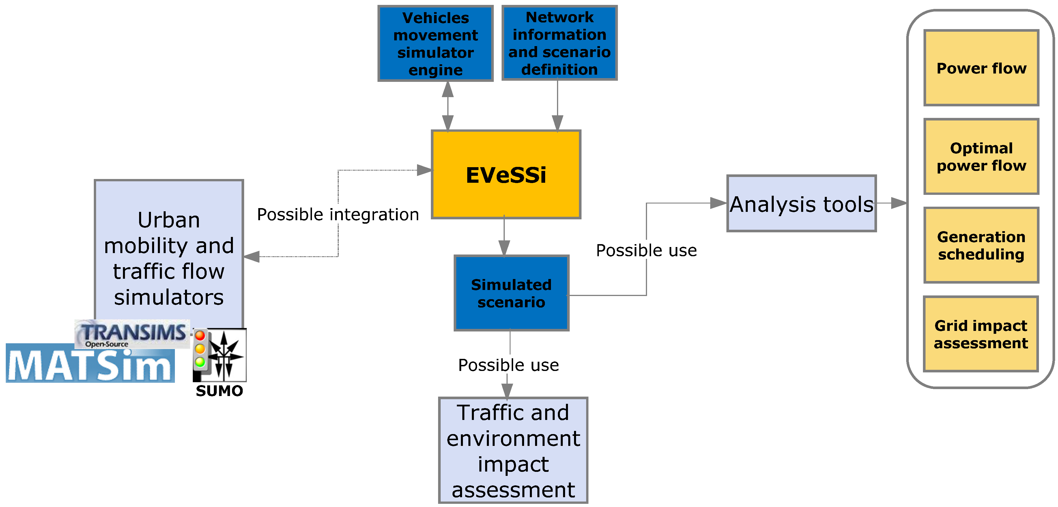
Figure 1 illustrates how EVeSSi tool is currently positioned between the transportation flow simulators and power systems tools. The EVeSSi receives as inputs the scenario definition regarding the electric vehicles’ characteristics and behaviour as well as distribution network information. The output of EVeSSi is a simulated scenario using its own developed movement simulator engine. The output of the EVeSSi, i.e., the simulated scenario, could be used with external tools, for instance, to analyse network impacts. In the future realistic and advanced movement simulator engine could be used, e.g., integrating with existing advanced traffic flow simulators. The integration of EVeSSi with a traffic simulator tool (transportation infrastructure) would eliminate the use of the EVeSSi’s movement simulator engine (top left blue module on Figure 1).

Figure 1. Electric Vehicle Scenario Simulator (EVeSSi) application framework.

Figure 1. Electric Vehicle Scenario Simulator (EVeSSi) application framework.

Instead, information using traffic mobility simulator would be gathered, e.g., location/zones of cars, parked cars, types of cars (EVs non-EVs), etc. The primary use of EVeSSi would be to define the distribution network infrastructure and EVs definitions. Grid geographical locations in the urban region would have to be defined, for instance defining that a given street with EVs charging points is electrically connected to the bus number “20” of distribution grid. The dependency of electricity grid on the future transportation systems is inevitable with the penetration of EVs. Adequate support and planning tools will be important for several study areas. With the integration of such tools it would be possible to provide accurate assessments on grid, environment and even on mobility impacts, for instance, taken into account that only EVs could access restricted streets/zones of the city/urban region has it happens in some cities already.

2. Electric Vehicles in Smart Grids

Electric vehicles (EVs) and Plug-in Hybrid Electric Vehicles (PHEV) are getting attention from most of the car makers around the world and are expected to be mass introduced. Inevitably this will cause impact to distribution systems networks and system operators [14]:

• A large number of PHEVs and EVs connected to the grid at the same time may pose a huge challenge to the power quality and stability of the overall power system [15].
• Due to some technical and economic issues, vehicle-to-grid is still less likely to become a reality in the short term [16].
• Effective communications technologies will be extremely important to the successful rollout of EVs [17].

Table 1 provides a summary of the battery specifications of the models presented in the MERGE review report [18]. This data provide support for EV battery modeling and enable the creation of different scenarios based on Battery Electric Vehicles (BEVs), PHEVs and Extended Range Electric Vehicles (EREVs). Vehicle classes from M1 to N1 in the table correspond to the ones defined by the European Commission [19]. It can be seen that the present EREVs models in the market do not allow the fast charge mode. The typical slow charge rate mode is 3 kW for the majority of classes presented. N2 class vehicles present a higher slow charge rate mode of 10 kW because the battery capacity tends to be much larger than normal passenger vehicles [18]. In spite of different charge rates between vehicle classes, 80% of EV’s potential users answered in a survey that the preferred charging place would be at home [18]. This means that the slow charge rate, which is available at home, is likely to be often used.

Table 1. EV battery specifications [18].

Vehicle class		Battery capacity (kWh)			Charging rates (kW)
		Max	Mean	Min	Slow charge rate	Fast charge rate
BEV	M1	72	29	10	2–8.8	3–240
	N1	40	23	9.6	1.3–3.3	10–45
	N2	120	85	51	10	35–60
	L7e	15	8.7	3	1–3	3–7.5
PHEV	M1	13.6	8.2	2.2	3	11
	N1	13.6	8.2	2.2	3	11
EREV	M1	22.6	17	12	3–5.3	-
	N1	22.6	17	12	3–5.3	-

Table 1. EV battery specifications [18].

Vehicle class		Battery capacity (kWh)			Charging rates (kW)
		Max	Mean	Min	Slow charge rate	Fast charge rate
BEV	M1	72	29	10	2–8.8	3–240
	N1	40	23	9.6	1.3–3.3	10–45
	N2	120	85	51	10	35–60
	L7e	15	8.7	3	1–3	3–7.5
PHEV	M1	13.6	8.2	2.2	3	11
	N1	13.6	8.2	2.2	3	11
EREV	M1	22.6	17	12	3–5.3	-
	N1	22.6	17	12	3–5.3	-

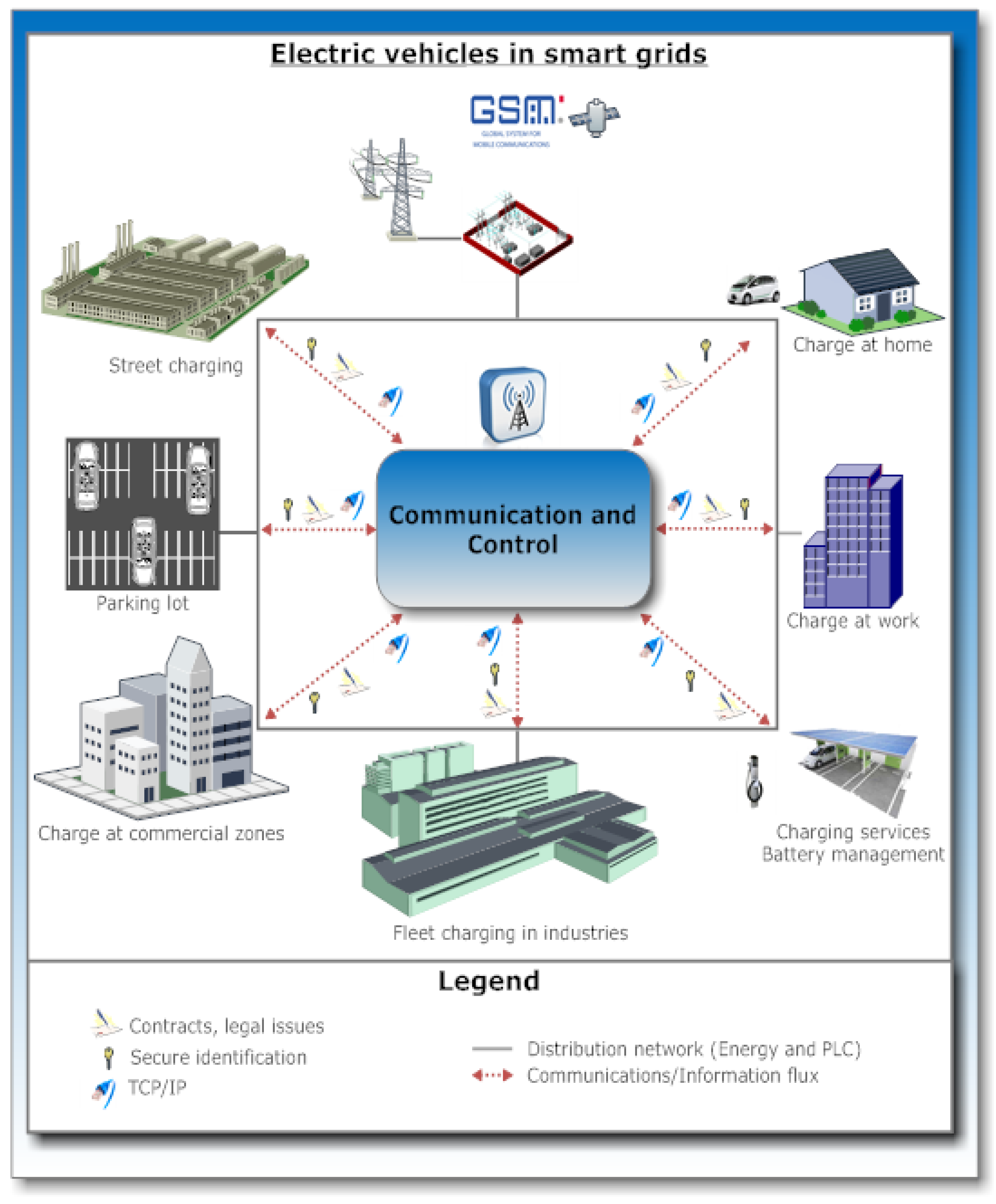
Figure 2 shows a representation of the interaction between electric vehicles and the electric grid in a smart grid environment. The communications technologies will be important as previously stated [17].

Figure 2. Electric vehicles in smart grids context. It shows a representation of the interaction between electric vehicles and the electric grid in a smart grid environment.

Figure 2. Electric vehicles in smart grids context. It shows a representation of the interaction between electric vehicles and the electric grid in a smart grid environment.

Adequate tools to provide realistic simulation, when considering EVs in the urban mobility context, are important to study, address and mitigate related problems with their presence. EVeSSi tool presented in this paper focuses on the consideration of the EVs’ mobility considering the electricity grid, thus it considers the network information, charging locations in each bus and roads data. EVeSSi enables to create custom tailored EV scenarios in a flexible and rapid way.

2.1. Driving Behaviour

The driving patterns are important because the impact on the power system depends on where and when the vehicles are charging, which affects the energy costs. Let us consider a typical daily drive for a person: starting from his/her house, then going to work, maybe the person has lunch in another place, comes back home and/or makes a detour to the store. This means that during the day the vehicle can be in different places: for instance in the garage, in an employer’s parking lot, a store parking lot and on the road. The main issue is to know where and when will the EV charge the battery and how many of them will do it simultaneously. This behaviour must be studied in order to allow an adequate resource management. Controlled charging of EV can help to reduce consumption impacts on the grids [20,21]; however, good control strategies must be implemented to avoid secondary system peaks.

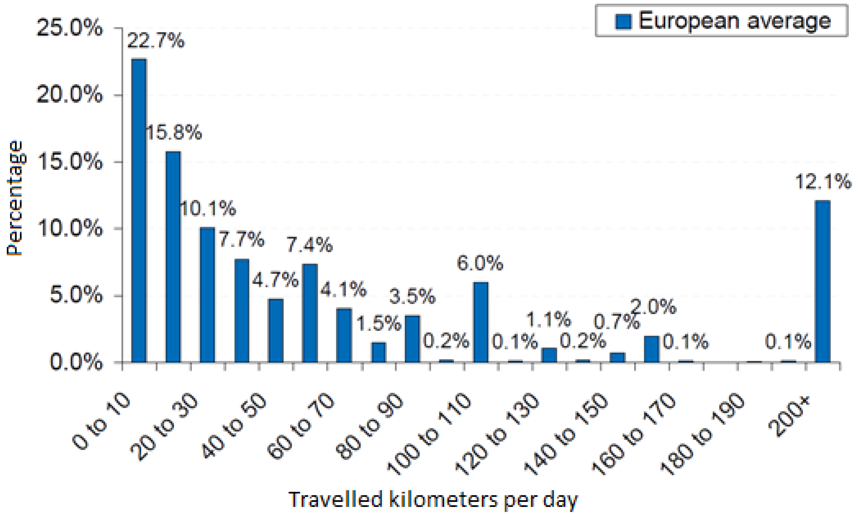
In the U.S. nearly 50% of Americans drive less than 42 km per day and 90% drive less than 150 km per day [22]. In Western Europe Cities (WEU), these values are lower: an average of 41 km driven per capita, per day and per vehicle in European cities contrasting with 85 km in the US cities [23] (see Figure 3). 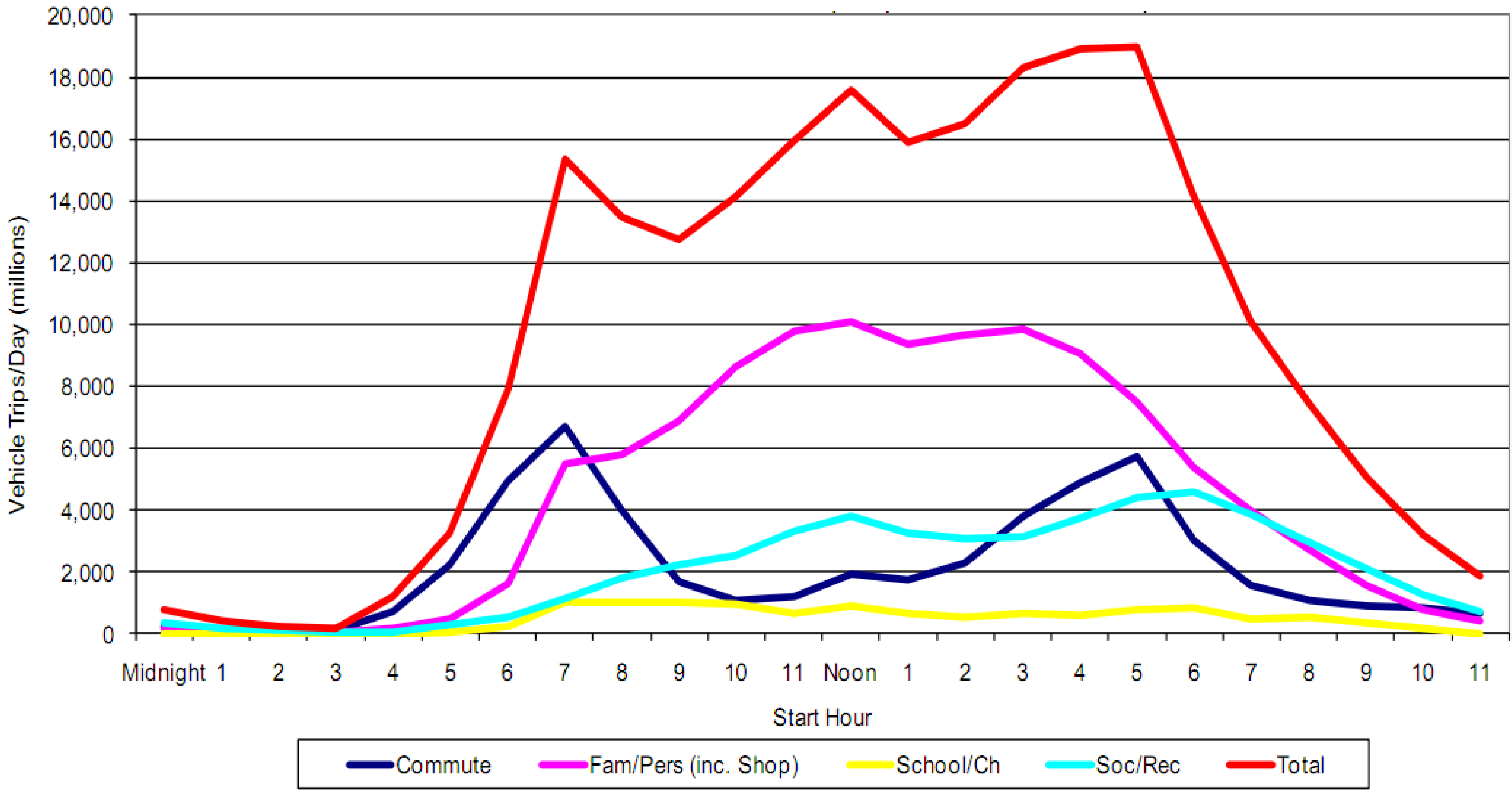Thus, the EVs in general have the potential to meet almost America's daily automotive transportation and certainly WEU cities regular needs on batteries alone, considering that most future commercial EVs will have more than 150 km of vehicle range [18]. In 2009, the U.S. Department of Transportation studied the percentage of trips in a day, and the results have shown that almost all cars are parked at night [24] (see Figure 4).

Figure 3. European average travelled per day on weekday [18].

Figure 3. European average travelled per day on weekday [18].

Figure 4. Distribution of vehicle trips by trip purpose and start [24].

Figure 4. Distribution of vehicle trips by trip purpose and start [24].

3. EVeSSi Framework

In this section the EVeSSi tool parameters and algorithm is described. This tool allows the creation of different scenarios in distribution networks, thus enabling a fast and organized way to deploy different case studies. The EV scenarios case studies presented in this paper were created using this tool.

3.1. EVeSSi Parameters

EVeSSi enables to create EV custom tailored scenarios in a flexible and rapid way. This section presents the parameters used by EVeSSi, which are organized in the following way: global parameters, trip parameters, EV classes and types parameters, and EV specific model parameters.

Table 2 presents the EVeSSi global parameters. These parameters are related to general considerations of the scenario. For instance, the value of chargingEfficiency, batteryEfficiency, initialStateOfBats, batteryMaxDoD parameters are applied to every EV present in the scenario. This is the default setting although these parameters can be applied individually. The recommended values according to [18] are 90% and 85% for chargingEfficiency and batteryEfficiency, respectively.

Table 2. EVeSSi global parameters.

Parameter	Description	Example value
initialStateOfBats	Initial state of batteries	30%
stepRate	Simulation time step (30 min, 1 hour)	1 hour
totalStep	Total number of steps (periods)	24
batteryMaxDoD	Battery max. depth of discharge permitted (DoD)	80%
chargingEfficiency 1	Slow charge mode efficiency	90%
chargingEfficiency 2	Fast charge mode efficiency	90%
batteryEfficiency	Battery efficiency	85%
evNum	Number of electric vehicles	2000
sameInitalEndBusProb	Probability of the EV to end in the same starting network bus in the simulation scenario	85%
parkedAllDay	Cars percentage that are always parked and connected to the grid	1%
carsInsideNetwork	Cars percentage that remain inside distribution network	50%
carsGoingOutsideNetwork	Cars percentage that leave distribution network	25%
carsGoingInsideNetwork	Cars percentage that arrive from other distribution network	25%

Table 2. EVeSSi global parameters.

Parameter	Description	Example value
initialStateOfBats	Initial state of batteries	30%
stepRate	Simulation time step (30 min, 1 hour)	1 hour
totalStep	Total number of steps (periods)	24
batteryMaxDoD	Battery max. depth of discharge permitted (DoD)	80%
chargingEfficiency 1	Slow charge mode efficiency	90%
chargingEfficiency 2	Fast charge mode efficiency	90%
batteryEfficiency	Battery efficiency	85%
evNum	Number of electric vehicles	2000
sameInitalEndBusProb	Probability of the EV to end in the same starting network bus in the simulation scenario	85%
parkedAllDay	Cars percentage that are always parked and connected to the grid	1%
carsInsideNetwork	Cars percentage that remain inside distribution network	50%
carsGoingOutsideNetwork	Cars percentage that leave distribution network	25%
carsGoingInsideNetwork	Cars percentage that arrive from other distribution network	25%

Table 3 presents the trip parameters. It is possible to define the distribution of trips along each period to simulate real-world conditions; for instance, using data supplied from [24] (Figure 4). The same is applied to define trip distance distribution (see Figure 3).

Table 3. EVeSSi trip parameters.

Parameter	Description
Trip distribution by period	Distribution of trips by each period
Trip distance distribution	Distribution of travelled distance

Table 3. EVeSSi trip parameters.

Parameter	Description
Trip distribution by period	Distribution of trips by each period
Trip distance distribution	Distribution of travelled distance

Table 4 presents the parameters related to the definition of vehicle classes and types. Recalling Table 1 of vehicles classes, it is possible to define the desired classes using EVeSSi parameters and setting classes distribution of the car fleet according to the aimed values, e.g., 90% of class M1 and 10% of class N2. Vehicle types and their distribution on the scenario can also be defined, e.g., 50% BEV and 50% PHEV. The tool accepts any number of vehicles types as well as vehicles classes.

Table 4. EVeSSi classes and types parameters.

Parameter	Description
Vehicle classes	Specification of vehicles classes present in the network
Vehicle classes distribution	Distribution of vehicle classes
Vehicle types	Specification of vehicles types present in the network
Vehicle types distribution	Distribution of vehicle types

Table 4. EVeSSi classes and types parameters.

Parameter	Description
Vehicle classes	Specification of vehicles classes present in the network
Vehicle classes distribution	Distribution of vehicle classes
Vehicle types	Specification of vehicles types present in the network
Vehicle types distribution	Distribution of vehicle types

Table 5 presents specific EV model parameters. The tool enables to specify any number of desired models. The parameters that are available for each model are depicted in the table. The parameter average km day, when supplied, overrides the average of trip distance distribution parameter (see Table 3), however a similar pattern distribution is adjusted to the average km day parameter.

Table 5. EVeSSi EV model parameters.

Parameter	Example value
Battery capacity	29 kWh
Slow charging rate	3 kW
Fast charging rate	57 kW
Average economy	0.16 kWh/km
Average km day	38 km
Average speed	35 km/h
Vehicle type	Plug-in hybrid vehicle
Vehicle class	M1
Tank capacity (hybrid models)	40 l
Consumption in hybrid mode	5 l/100km
Trip time in hybrid mode	20%

Table 5. EVeSSi EV model parameters.

Parameter	Example value
Battery capacity	29 kWh
Slow charging rate	3 kW
Fast charging rate	57 kW
Average economy	0.16 kWh/km
Average km day	38 km
Average speed	35 km/h
Vehicle type	Plug-in hybrid vehicle
Vehicle class	M1
Tank capacity (hybrid models)	40 l
Consumption in hybrid mode	5 l/100km
Trip time in hybrid mode	20%

3.2. EVeSSi Algorithm

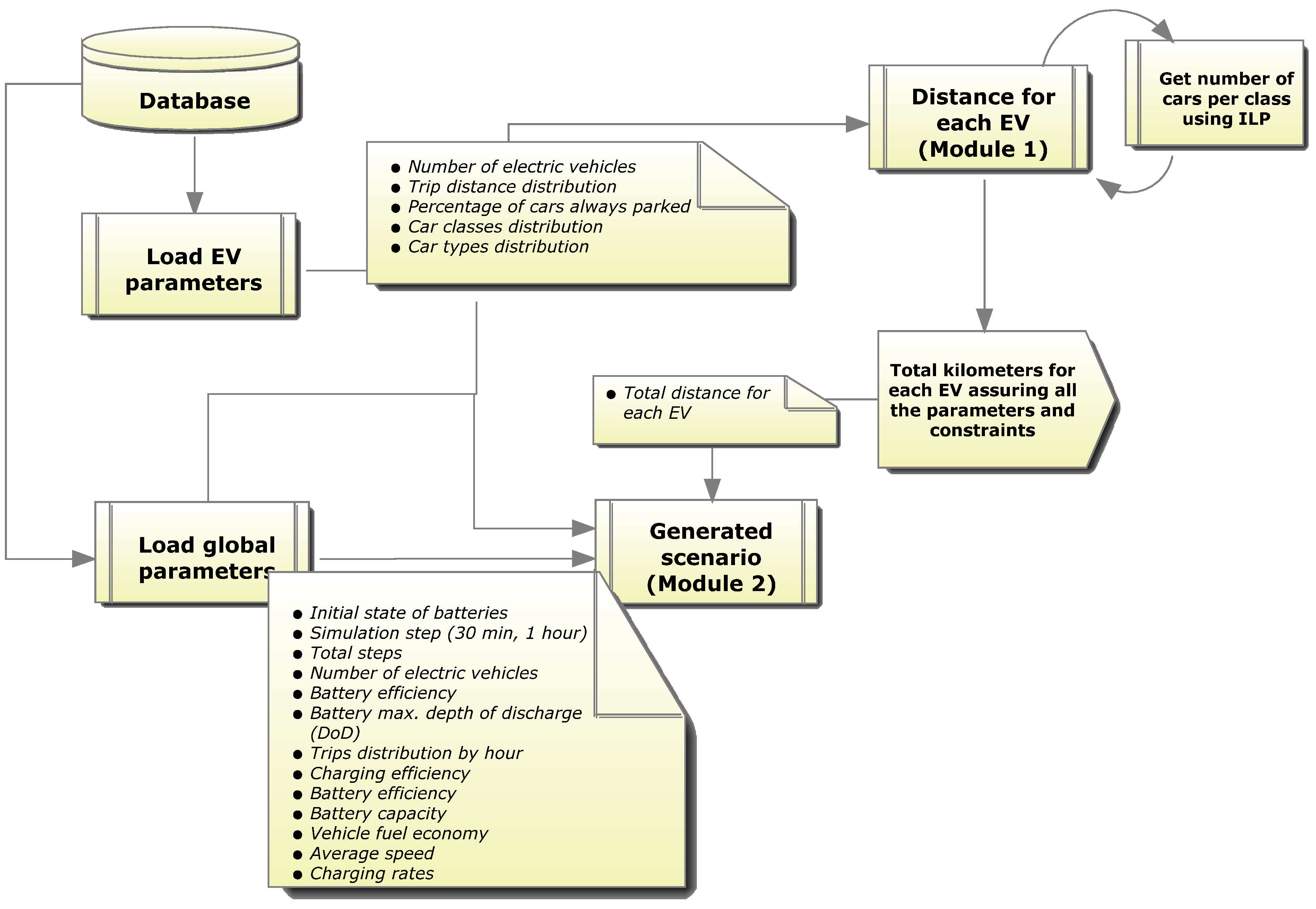
A schematic view of the process used by EVeSSi to create a given scenario is presented in Figure 5. The parameters described in subsection 3.1 are supplied to EVeSSi using a database. In the figure, two main models can be identified:

• Distance for each EV;
• Generated scenario.

The parameters required by each module are highlighted within a label. In the figure only EV and global parameters appear due to figure size restriction. However, all the parameters described in 3.1 are loaded from the database.

In module 1—Distance for each EV—a sub-module to calculate the number of cars of each model was developed. This sub-module intends to guarantee user defined parameters and the mathematical formulation uses an Integer Programming (IP) model. The objective function is neutral (0–neither minimizing nor maximizing the objective function) because the reason of using IP method in this sub-module is to guarantee problem constraints. These constraints depend on the defined parameters. This sub-module will return the number of cars per each defined model (see Table 5) according to classes and types parameters (Table 3).

Figure 5. EVeSSi framework.

Figure 5. EVeSSi framework.

The mathematical model is defined below:

$$Min.f={\displaystyle \sum }_{i=1}^{modelNum}{x}_i\times 0$$

(1)

subject to the following constraints:

$${\displaystyle \sum }_{i=1}^{modelNum}{x}_i=evNum$$

(2)

$${\displaystyle \sum }_{j=1}^{techTypesNum}{\displaystyle \sum }_{i\in techTypeSe{t}_j}^{}{x}_i=evNum\times techWeigh{t}_j$$

(3)

$${\displaystyle \sum }_{k=1}^{classesNum}{\displaystyle \sum }_{i\in classesSe{t}_j}^{}{x}_i=evNum\times classesWeigh{t}_k$$

(4)

where:

• $classesNum$ is total number of classes available
• $classesSe{t}_j$ is the set of model types i that belong to class j
• $classesWeigt{h}_j$ is the weight for class type j (e.g., 90% passenger vehicles, 10% commercial vehicles)
• $evNum$ is the total number of electric vehicles including all models
• $smodelNum$ is the total number of models available
• $techTypesNum$ is the total number of technology types available
• $techTypeSe{t}_j$ is the set of model types i that belong to tech type j
• $techWeigt{h}_j$ is the weight for technology type j (e.g., 40% BEV, 60% PHEV)
• $x_i$ is an integer variable where each $x_i$ represents the number of vehicles of model i

With the information returned by the sub-module, module 1—Distance for each EV—will use EV parameters (see Table 5) and trip distance distribution parameters (see Table 3) to calculate the total distance allocated to each EV. Also in this module, the carsParkedAllDay parameter (Table 2) is used for setting some cars to be parked all day. Module 1—Distance for each EV—will return the total distance for each EV.

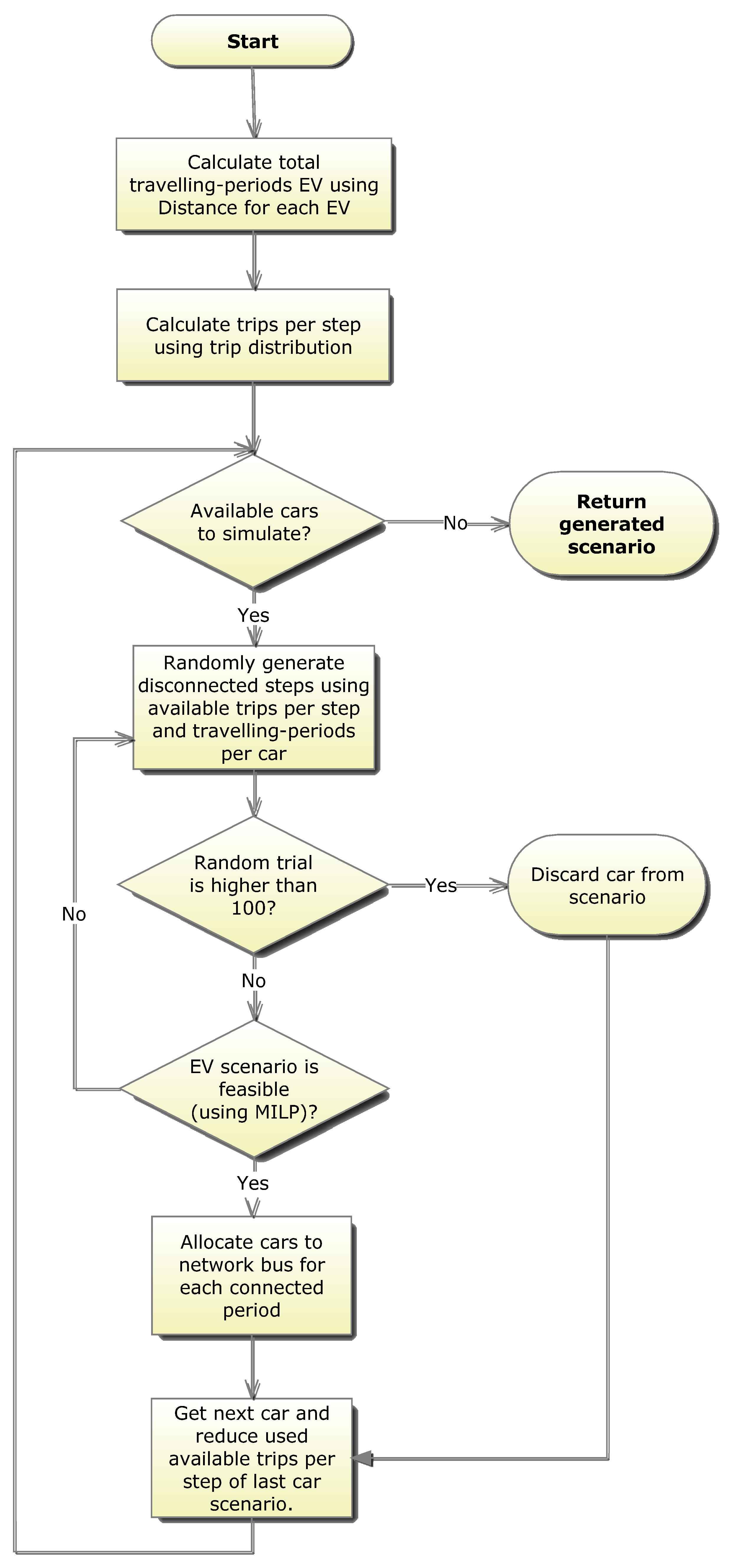
Module 2—Generated scenario—depends on the result of module 1. With the EVs’ distance information returned by the first module, an attempt is made to create a scenario. Figure 6 presents a flowchart of the algorithm that is the basis of module 2. Travelling-periods are calculated using the distance for each EV returned by module 1. This value corresponds to the number of periods that each vehicle will be disconnected from the grid for travelling purposes. As an example, if the distances returned by module 1 for vehicle 1 and vehicle 2 are 10 km and 50 km, respectively, using average speed parameter for the corresponding model of each vehicle (see Table 5), assuming 35 km/h for both vehicles, then the travelling-periods would be 1 and 2 for vehicle 1 and 2, respectively, considering a time step of 1 hour, i.e., ceiling the result to the nearest integer of the divisions 10/35 and 50/35. If vehicle 1 distance was 35 km and the average speed parameter the same 35 km/h the corresponding travelling-periods would also be 1, however, the energy consumption during the disconnected period would be different.

In this stage, there is only the information of the number of traveling-periods (disconnected periods) for each EV. The next step of the algorithm is to calculate the number of trips that will occur in each period using travelling-periods information and trip distribution by period (see Table 3) resulting in a vector with the information of scenario trips number per period.

After that, with the number of trips per period, the algorithm will attempt different disconnected period possibilities. For example, if vehicle 2 has two travelling-periods, then the algorithm randomly allocates these two travelling-periods to the available number of periods, for instance, periods 8 and 18. This guarantees the trip distribution by period parameter. Mixed Integer Linear Programming (MILP) is used to ensure feasibility of the randomly generated EV disconnected scenario.

Figure 6. Module 2 algorithm flowchart.

Figure 6. Module 2 algorithm flowchart.

The objective function minimizes the use of fast charge in order to avoid early battery wear-out. If a feasible solution is found using MILP, the disconnected scenario is accepted for the given EV; otherwise, another randomly disconnected scenario is attempted. In the case of continued failed trials, the EV is marked as infeasible on the network and discarded from the scenario. The mathematical formulation of the feasibility check is defined as follows:

$$Min.f={\displaystyle \sum }_{i=1}^T{Y}_t$$

(5)

Subject to the following constraints:

$$E_{Stored\left(t\right)}=initialBatState,witht=0$$

(6)

$$E_{Stored\left(t\right)}=E_{Stored\left(t-1\right)}+E_{Charge\left(t-1\right)}-E_{Trip\left(t-1\right)},\forall t\in \{1,\dots ,T\}$$

(7)

$$E_{Trip\left(t\right)}*Z_t-E_{Stored\left(t\right)}\le 0$$

(8)

$$E_{Stored\left(t\right)}\le batCap,\forall t\in \{1,\dots ,T\}$$

(9)

$$E_{Charge\left(t\right)}=n_{slowCharge}*P_{SlowChargeRate\left(t\right)}*X_t*\Delta cd+n_{fastCharge}*P_{FastChargeRate\left(t\right)}*Y_t*\Delta cd,\forall t\in \{1,\dots ,T\}$$

(10)

$$X_t+Y_t+Z_t\le 1,\forall t\in \{1,\dots ,T\}$$

(11)

where:

• $\Delta cd$ is the duration of charging, typically $\Delta t=1$
• $n_{slowCharge}$ is the charging efficiency in slow charge mode
• $n_{fastCharge}$ is the charging efficiency in fast charge mode
• $batCap$ is the limit of battery capacity
• $E_{Charge\left(t\right)}$ is the energy charged in period t
• $E_{Stored(t)}$ is the battery’s energy stored in period t
• $E_{Trip(t)}$ is the energy consumed by vehicle trip in period t
• $initialBatState$ is the initial battery state of the battery
• $P_{FastChargeRate\left(t\right)}$ is the fast charge rate in period t
• $P_{SlowChargeRate\left(t\right)}$ is the slow charge rate in period t
• $T$ is the number of periods
• $X_t$ is the slow charge binary variable in period t
• $Y_t$ is the fast charge binary variable in period t
• $Z_t$ is a Boolean for trip decision in period t (0/1) and fixed before optimization

4. Experimental Cases

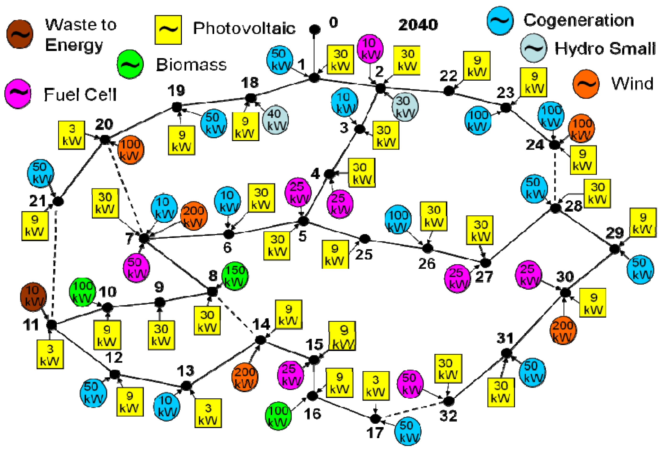
In this section, two experimental case studies are presented using the EVeSSi tool. The first case study uses a 33 bus distribution network [25,26,27] (see Figure 7) with 2000 electric vehicles and the second case study uses a 937 bus distribution network with 15,000 electric vehicles.

General parameters of the simulated scenarios are given in Table 6. The distribution of trips along the day are based on the data provided in [24] (see Figure 4). The data concerning vehicle definition are listed in Table 7 to Table 9. Table 7 considers the data regarding the parameters considered for the eight model types (four BEVs, two PHEVs and two EREVs). Table 8 shows the distribution considered for the vehicles classes. These definitions in the first scenario correspond to: 10 vehicles of L7e, 1740 of M1, 200 of N1 and 50 of N2 totaling 2000 vehicles. Table 9 presents the EV types distribution. Identical share of about 33% for EVs types were assumed in the scenario, e.g., for BEV, PHEV and EREV types.

Figure 7. 33 bus distribution network configuration scenario [25,26,27].

Figure 7. 33 bus distribution network configuration scenario [25,26,27].

Table 6. Scenario parameters.

	Parameter value
Battery efficiency	85%
Cars parked all day (no movements)	1%
Charging efficiency (slow and fast mode)	90%
Initial state of battery	30%
Maximum depth of discharge	80%
Number of EVs	2000
Number of periods	24
Time step	1 hour

Table 6. Scenario parameters.

	Parameter value
Battery efficiency	85%
Cars parked all day (no movements)	1%
Charging efficiency (slow and fast mode)	90%
Initial state of battery	30%
Maximum depth of discharge	80%
Number of EVs	2000
Number of periods	24
Time step	1 hour

Table 7. Vehicle model definitions.

Model ID	Description	Battery capacity (kWh)	Slow charging rate (kW)	Fast charging rate (kW)	Average economy (kWh/km)	Average speed (km/h)	Average km day (km/day)	Vehicle type	Vehicle class
1	Passenger car	8.7	3	0	0.1122	20	20	BEV	L7e
2	Passenger car	28.5	3	57	0.1608	35	38	BEV	M1
3	Commercial van	23.0	3	46	0.1854	30	56	BEV	N1
4	Light truck	85.3	10	60	0.5867	40	136	BEV	N2
5	Passenger car	8.2	3	0	0.1560	35	20	PHEV	M1
6	Commercial van	8.2	3	0	0.1560	30	20	PHEV	N1
7	Passenger car	16.9	3	0	0.2530	35	20	EREV	M1
8	Commercial van	16.9	3	0	0.2530	30	30	EREV	N1

Table 7. Vehicle model definitions.

Model ID	Description	Battery capacity (kWh)	Slow charging rate (kW)	Fast charging rate (kW)	Average economy (kWh/km)	Average speed (km/h)	Average km day (km/day)	Vehicle type	Vehicle class
1	Passenger car	8.7	3	0	0.1122	20	20	BEV	L7e
2	Passenger car	28.5	3	57	0.1608	35	38	BEV	M1
3	Commercial van	23.0	3	46	0.1854	30	56	BEV	N1
4	Light truck	85.3	10	60	0.5867	40	136	BEV	N2
5	Passenger car	8.2	3	0	0.1560	35	20	PHEV	M1
6	Commercial van	8.2	3	0	0.1560	30	20	PHEV	N1
7	Passenger car	16.9	3	0	0.2530	35	20	EREV	M1
8	Commercial van	16.9	3	0	0.2530	30	30	EREV	N1

Table 8. EV classes definition.

Vehicle class	Share
L7e	0.005
M1	0.870
M2	0.000
M3	0.000
N1	0.100
N2	0.025
N3	0.000

Table 8. EV classes definition.

Vehicle class	Share
L7e	0.005
M1	0.870
M2	0.000
M3	0.000
N1	0.100
N2	0.025
N3	0.000

Table 9. EV types definition.

Vehicle type	Share
BEV	0.333
PHEV	0.333
EREV	0.333

Table 9. EV types definition.

Vehicle type	Share
BEV	0.333
PHEV	0.333
EREV	0.333

The stats resulting from the use of EVeSSi tool for the first scenario are shown in Table 10. Execution time was about 40 seconds for the entire 24 hours simulation. The average distance travelled by car was 29 km and the maximum distance travelled by a car was 482 km whereas the minimum was 0 (some cars remained parked during the entire day). Therefore, the total distance accumulated by the 2000 cars was 58,438 km corresponding to a battery energy use of 13,306 kWh.

Table 10. Scenario stats 33 bus network.

		Driving stats
Total number of cars		2000
Total trip distance (km)	Cars average	29
	Maximum	482
	Minimum	0
Total distance (km)		58,438
Total energy consumption (kWh)		13,306
Mean battery capacity (kWh)		19
Algorithm execution time		40 seconds

Table 10. Scenario stats 33 bus network.

		Driving stats
Total number of cars		2000
Total trip distance (km)	Cars average	29
	Maximum	482
	Minimum	0
Total distance (km)		58,438
Total energy consumption (kWh)		13,306
Mean battery capacity (kWh)		19
Algorithm execution time		40 seconds

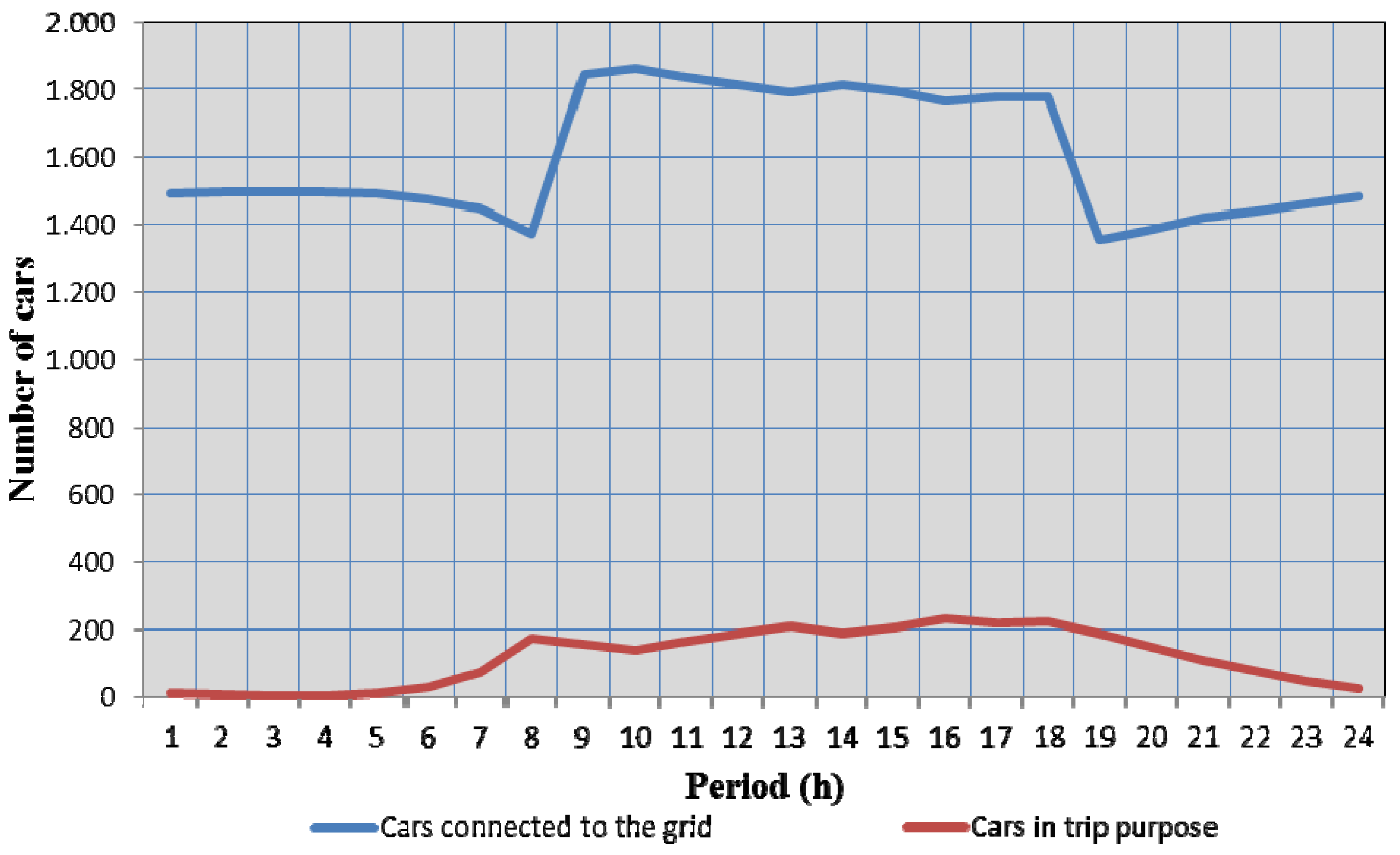
To simulate movements to and from the considered network, it was assumed that 50% of the cars remained inside the network, i.e., 1,000 cars, 25% of cars remained inside the network from 9 a.m. to 18 p.m. and 25% from 19 p.m. to 8 a.m. The outcome of simulated movements during the simulation time using such assumptions is expressed in Figure 8. This figure presents the total number of cars connected to the electricity grid and the number of cars in trip purpose as simulated by EVeSSi. 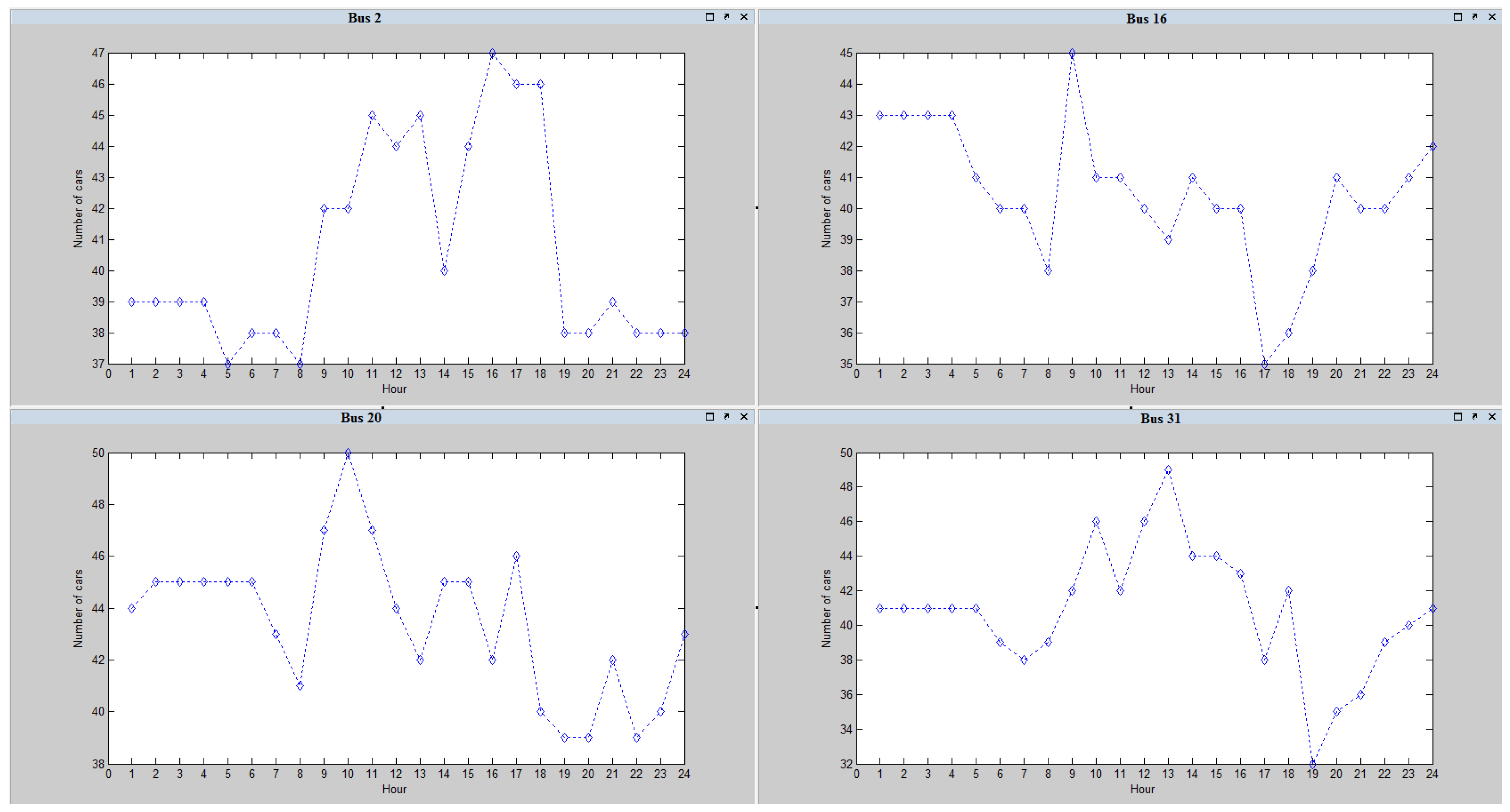Figure 9 presents the total number of cars for some selected buses, namely bus 2, 16, 20 and 31.

Figure 8. Cars connected to the grid. Blue line presents the total number of cars connected to the grid and the red line the total number of cars in trip purpose as simulated by EVeSSi tool.

Figure 8. Cars connected to the grid. Blue line presents the total number of cars connected to the grid and the red line the total number of cars in trip purpose as simulated by EVeSSi tool.

Figure 9. Total number of EVs connected to Buses 2, 16, 20 and 31 during the simulation.

Figure 9. Total number of EVs connected to Buses 2, 16, 20 and 31 during the simulation.

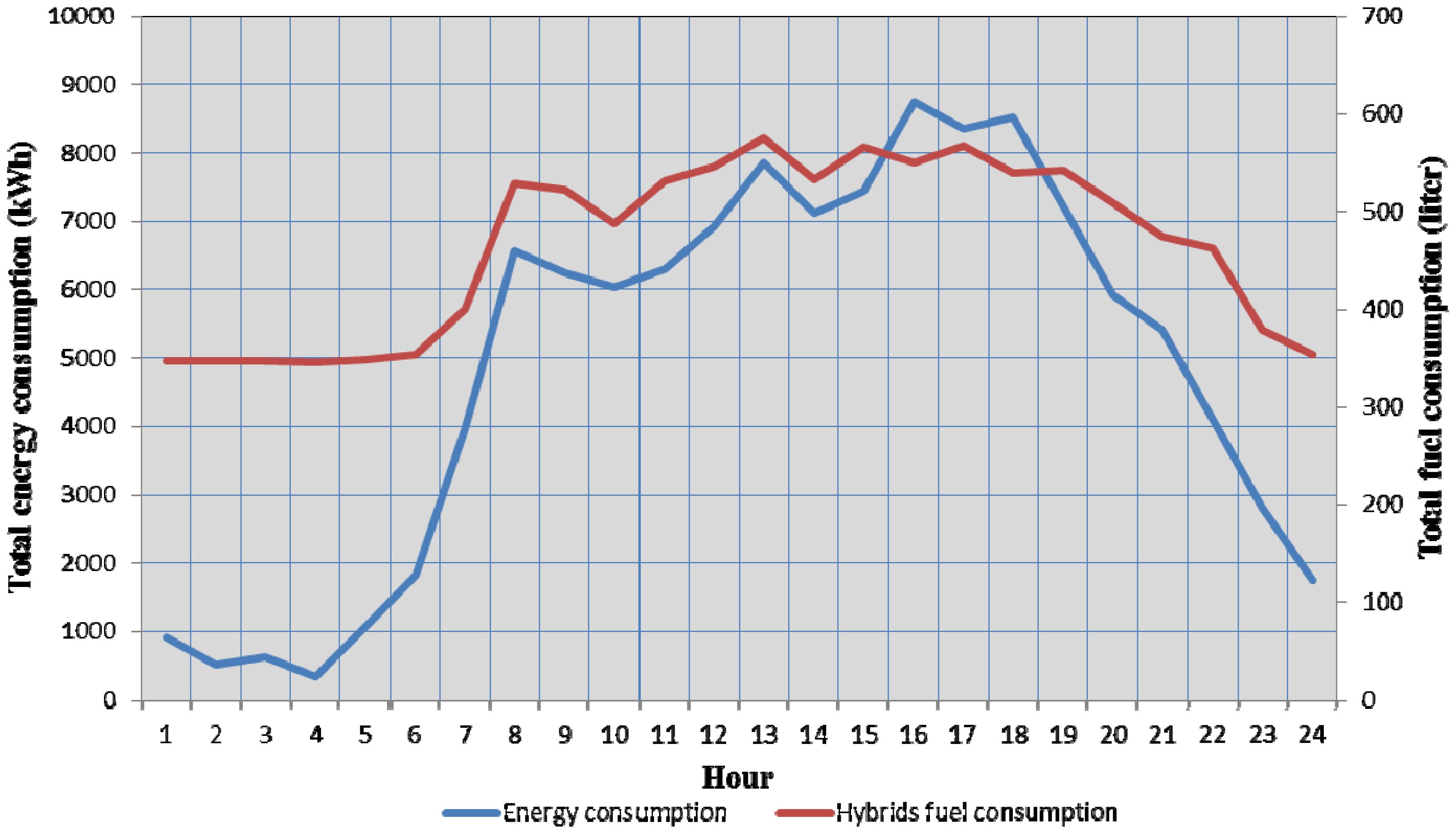
The second case study used the same parameters as described for scenario 1 with 2,000 vehicles (Table 6 to Table 9). However, this scenario used a 937 bus distribution system network with 15,000 vehicles. Table 11 depicts the results of the simulation test. Figure 10 shows the energy consumption and the total fuel consumption for hybrids (PHEVs and EREVs) of the simulation test. Comparing this scenario (Table 11) with the first one (see Table 10) the average travelled distance as well as the maximum travelled distance by a car changed slightly due to stochastic factors. The total distance simulated in this case was 499,670 km corresponding to a battery energy use of 116,596 kWh.

Table 11. Scenario stats 937 bus.

		Driving stats
Total number of cars		15,000
Total trip distance (km)	Cars average	33
	Maximum	535
	Minimum	0
Total distance (km)		499,670
Total energy consumption (kWh)		116,596
Mean battery capacity (kWh)		19
Algorithm execution time		352 seconds

Table 11. Scenario stats 937 bus.

		Driving stats
Total number of cars		15,000
Total trip distance (km)	Cars average	33
	Maximum	535
	Minimum	0
Total distance (km)		499,670
Total energy consumption (kWh)		116,596
Mean battery capacity (kWh)		19
Algorithm execution time		352 seconds

Figure 10. Energy and fuel consumption by hour during simulation for the 937 bus scenario with 15,000 EVs.

Figure 10. Energy and fuel consumption by hour during simulation for the 937 bus scenario with 15,000 EVs.

5. Conclusions and Future Work

The present paper describes a tool to simulate EVs in a distribution network that can be customized to accommodate different networks, types, and number of EVs. The EVeSSi is a new type of tool that bridges the new dependency between electric vehicle transportation and urban mobility with the electricity network. A fast algorithm model is considered to simulate the EVs’ movements in the network and potentially allowing estimation of the impacts of charging in each bus of the system, the energy consumption in a given scenario, the emissions and so on. The EVeSSi tool will be further enhanced to implement advanced parameters such as the road network information where the electricity network belongs. This will enable realistic car movements and accurate distances between trip places. Also in the future version of EVeSSi the slope of the roads will be used to increase the overall accuracy of battery use. Switch battery stations and induction charging places will be considered in future versions of EVeSSi as well. Furthermore, it is planned to have a fully developed interface and a 3D visualization module. The authors aim to integrate the features of EVeSSi with an advanced traffic simulator such as SUMO or develop its own traffic simulation model.

This will catch both areas of transportation and energy systems with benefits for both areas and completing each other with its integration in the same simulator. The possible users for this tool can be: electricity network operators, energy analysts, urban mobility planners and city planners.