1. Introduction
Carbon dioxide has contributed to more than 70% of total greenhouse gas concentration in the atmosphere leading to the deleterious effect from climate change and global warming. Due to economic development and population increase, electricity demand growth in developing countries has lead to increasing CO
2 emissions in the power sector. Although CO
2 emission reduction for developing countries has not been targeted by the Kyoto Protocol [
1], the power generation expansion planning (PGEP) for both developed and developing countries needs to be concerned about providing efficient power generation to satisfy the electricity demand. Environmental protection is also a serious challenge in power system development [
2]. Thailand is also concerned with such a problem, especially in the power sector. Two important plans, the 20-year National Energy Conservation Plan (NCEP) of 2011–2030 and the 15-year Alternative Energy Development Plan (AEDP) of 2008–2022, were launched and associated with CO
2 emission mitigation from electricity production. Based on the efficiency improvement of energy utilization and avoidance of unnecessary consumption, the NECP has been assessed its own potential to save electricity consumption of 86,150 GWh in three economic sectors: industrial, commercial and residential sectors [
3]. Meanwhile, the primary purpose of AEDP is to promote renewable energy utilization. The total installed capacity of renewable energy is targeted up to 5608 MW which would produce 26,500 GWh of power generation by the year 2022. Additionally, subsidies in the form of “adders” within certain time periods for particular renewable energy technologies are established to promote investment of renewable power generation [
4].
The objective of the paper is to assess the impact of two important policy drivers proposed by the Thai government on the Thai power supply sector with the help of Mixed Integer Linear Programming (MILP). These two policy drivers are Energy Efficiency and Renewable Energy. The impact of constraints with regard to CO2 emissions and the various power generation technologies on future technology selection have been assessed. In this study, the least-cost PGEP model was developed on the basis of General Algebraic Modeling System (GAMS) framework which provides Cplex, the well-known MILP solver in order to select the optimal capacity expansion and generation mix under different scenarios during 2010–2030. In this study the specific CO2 emission reduction targets are adopted as emission constraints in optimization. Financial and environmental impacts of NECP and AEDP are further assessed by the PGEP model. Different scenarios related to selected policies and CO2 emission reduction targets were conducted in order to analyze their own impacts in terms of cost savings, CO2 intensity as well as fuel imported requirement.
2. Mathematical Formulation of MILP Model in GAMS Framework
In this study, the PGEP model was operated on Pentium quad-core processor at a processing speed of 2.66 GHz with 3 GB of RAM based on the GAMS program, which provides ILOG Cplex 9.0 solver for handling MILP problem efficiently [
5]. In order to minimize the generation and expansion cost (
Objcost) by using the above mentioned model, the mathematical formulation of the objective function and its corresponding constraints must be a linear combination of mixed-integer decision variables as in the following expression:
The objective function to determine the investment cost (
It), salvage value (
St), fixed operation and maintenance cost (
Ft), variable operation and maintenance cost (
Vt) and total adder subsidy for renewable energy (
SDt) are as follows:
The integer decision variables, ui,t and ui,r represent the number of the ith candidate technology in the tth year and the rth year, respectively. The continuous decision variables, pi,s,t represents the power output of the ith candidate technology in the sth subperiod in the tth year and pj,s,t the power output of the jth existing technology in the sth subperiod in the tth year. The parameters Capi, Invi, δi, Fixedi and Vari, represent the capacity, investment, salvage value, fixed and variable operational maintenance charges of the ith candidate technology, respectively. The variable operational maintenance charge also includes the fuel cost. ExistCapj, Fixedj and Varj represent the capacity, fixed and variable operational maintenance charges of the jth existing technology, respectively. The constants D and K are the discount rate and number of hours in sub-period, respectively. EFi and EFj are the CO2 emission factors of the ith candidate technology and the jth existing technology. Adderi and TiSubsidy are adder costs and subsidy periods of the ith candidate technology, respectively.
Constraint handling is primary and requisite to optimization practice. The constraints normally entail the physical limitation of the realistic system. For the entire planning horizon, the total installed capacity in the power system must satisfy maximum and minimum reserve margin which are characterized by proportion of peak load in Equation (7). In each sub-period, total power generation of the selected existing and candidate generating units must be sufficient for the predicted electricity demand, along with Load Duration Curve (LDC) in Equation (8). Furthermore, the power generation by each existing and candidate unit must be limited by its capacity factor in Equations (9,10). Renewable energy utilization always encounters with limitation of resources. The conversion of particular renewable energy to electricity cannot exceed its own potential in Equation (11). Finally, CO
2 reduction target is imposed on constrained optimization Equation (12). The above mentioned mathematical constraints are formulated as follows:
where
Rmin and
Rmax denotes the minimum and maximum reserve margins, respectively.
CFi and
CFj denotes the capacity factors of the
ith candidate technology and the
jth existing technology respectively.
PREi denotes the maximum capacity expansion of the
ith candidate renewable energy technology.
Loadk,t denotes the load of the
kth sub-period in the
tth year and
Load1,t denotes the peak load in the
tth year.
LimitCO2 denotes the limitation of CO
2 emissions related to the reduction targets.
3. Description of Scenarios
In power system planning, the Electricity Generating Authority of Thailand (EGAT) is responsible for PGEP. The Power Development Plan 2010 (PDP2010) was thus formulated and served as the master plan to expand generation capacity. In this study the planning horizon of PGEP is the period between 2010 and 2030 according to the PDP2010 [
6]. A discount rate of 10% per year is used and the reserved margin is always maintained between 15% and 25%. The salvage value was set at 0.15 for all candidate technologies. The fuel price of natural gas, coal, lignite, fuel oil, diesel, uranium and biomass is 9.76, 4.01, 0.95, 14.3, 20.51, 0.5 and 2.01 $/MMBtu, respectively [
6,
7,
8]. With respect to future fuel prices, an escalation rate of 2.3% per year was applied according to prior work in [
9]. In this study, five scenarios of PGEP have been considered and their descriptions are as follows.
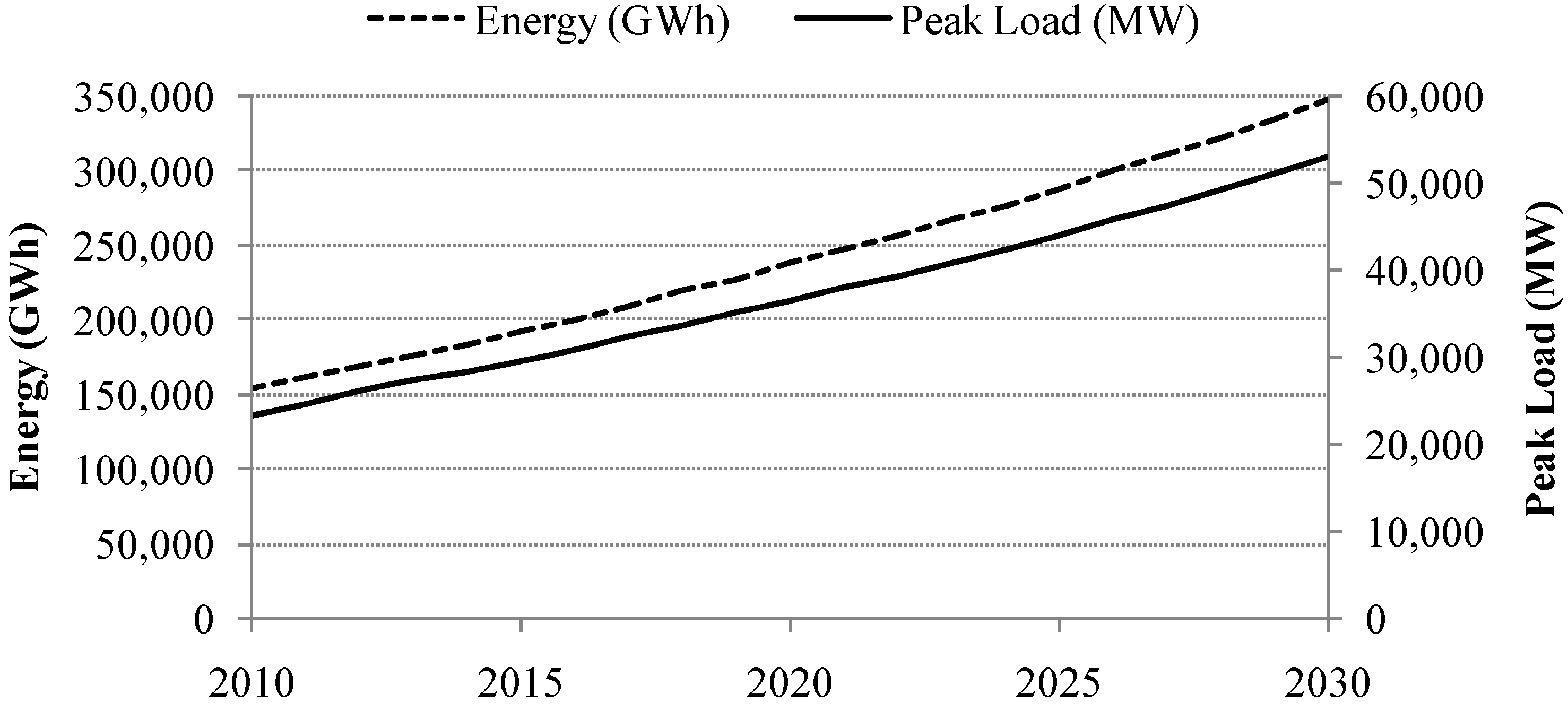
Business-as-usual scenario (hereafter referred to as “BAU”) is the reference scenario. The load duration curve (LDC) used in this study is presented in
Table 1. Each year of planning horizon is divided into 12 equal segments, and each contains 730 hours. The load levels in each segment are obtained from Thailand’s hourly electricity consumption in 2009 [
6]. The average load demand growth is about 4.27% per year. The electricity consumption is expected to increase from 144,791 GWh in 2009 to 347,947 GWh in 2030, as shown in
Figure 1.
Table 2 describes the replacement of existing power plants according to the retirement schedule. Nuclear power is initially introduced from 2020 and limited to only one unit per year according to PDP2010. Renewable power generation is constrained by its resource potentials with regard to the AEDP plan (see
Table 3).
Table 1.
Load profiles of in the PGEP model.
Table 1.
Load profiles of in the PGEP model.
| Year | Load factor | Sub-period |
|---|
| 1 | 2 | 3 | 4 | 5 | 6 | 7 | 8 | 9 | 10 | 11 | 12 |
|---|
| 2009 | 74.98 | 22,045 | 20,844 | 19,945 | 19,113 | 18,239 | 17,153 | 15,914 | 15,014 | 14,308 | 13,526 | 12,461 | 9,782 |
| 2010 | 75.1 | 23,249 | 21,751 | 20,852 | 20,020 | 19,146 | 18,060 | 16,821 | 15,921 | 15,215 | 14,433 | 13,368 | 10,690 |
| 2011 | 74.5 | 24,568 | 22,550 | 21,651 | 20,819 | 19,945 | 18,859 | 17,620 | 16,720 | 16,014 | 15,232 | 14,167 | 11,487 |
| 2012 | 74.03 | 25,913 | 23,389 | 22,490 | 21,658 | 20,784 | 19,698 | 18,459 | 17,559 | 16,853 | 16,071 | 15,006 | 12,324 |
| 2013 | 73.74 | 27,188 | 24,217 | 23,318 | 22,486 | 21,612 | 20,526 | 19,287 | 18,387 | 17,681 | 16,899 | 15,834 | 13,155 |
| 2014 | 73.89 | 28,341 | 25,086 | 24,187 | 23,355 | 22,481 | 21,395 | 20,156 | 19,256 | 18,550 | 17,768 | 16,703 | 14,026 |
| 2015 | 74.09 | 29,463 | 25,952 | 25,053 | 24,221 | 23,347 | 22,261 | 21,022 | 20,122 | 19,416 | 18,634 | 17,569 | 14,891 |
| 2016 | 74.24 | 30,754 | 26,929 | 26,030 | 25,198 | 24,324 | 23,238 | 21,999 | 21,099 | 20,393 | 19,611 | 18,546 | 15,868 |
| 2017 | 74.15 | 32,225 | 27,955 | 27,056 | 26,224 | 25,350 | 24,264 | 23,025 | 22,125 | 21,419 | 20,637 | 19,572 | 16,900 |
| 2018 | 74.15 | 33,688 | 29,004 | 28,105 | 27,273 | 26,399 | 25,313 | 24,074 | 23,174 | 22,468 | 21,686 | 20,621 | 17,948 |
| 2019 | 74.26 | 34,988 | 29,979 | 29,080 | 28,248 | 27,374 | 26,288 | 25,049 | 24,149 | 23,443 | 22,661 | 21,596 | 18,924 |
| 2020 | 74.44 | 36,336 | 31,022 | 30,123 | 29,291 | 28,417 | 27,331 | 26,092 | 25,192 | 24,486 | 23,704 | 22,639 | 19,964 |
| 2021 | 74.4 | 37,856 | 32,101 | 31,202 | 30,370 | 29,496 | 28,410 | 27,171 | 26,271 | 25,565 | 24,783 | 23,718 | 21,043 |
| 2022 | 74.49 | 39,308 | 33,184 | 32,285 | 31,453 | 30,579 | 29,493 | 28,254 | 27,354 | 26,648 | 25,866 | 24,801 | 22,122 |
| 2023 | 74.6 | 40,781 | 34,296 | 33,397 | 32,565 | 31,691 | 30,605 | 29,366 | 28,466 | 27,760 | 26,978 | 25,913 | 23,234 |
| 2024 | 74.81 | 42,236 | 35,448 | 34,549 | 33,717 | 32,843 | 31,757 | 30,518 | 29,618 | 28,912 | 28,130 | 27,065 | 24,392 |
| 2025 | 74.68 | 43,962 | 36,634 | 35,735 | 34,903 | 34,029 | 32,943 | 31,704 | 30,804 | 30,098 | 29,316 | 28,251 | 25,578 |
| 2026 | 74.76 | 45,621 | 37,877 | 36,978 | 36,146 | 35,272 | 34,186 | 32,947 | 32,047 | 31,341 | 30,559 | 29,494 | 26,818 |
| 2027 | 74.84 | 47,344 | 39,166 | 38,267 | 37,435 | 36,561 | 35,475 | 34,236 | 33,336 | 32,630 | 31,848 | 30,783 | 28,107 |
| 2028 | 75.06 | 49,039 | 40,511 | 39,612 | 38,780 | 37,906 | 36,820 | 35,581 | 34,681 | 33,975 | 33,193 | 32,128 | 29,455 |
| 2029 | 75.03 | 50,959 | 41,892 | 40,993 | 40,161 | 39,287 | 38,201 | 36,962 | 36,062 | 35,356 | 34,574 | 33,509 | 30,840 |
| 2030 | 75.1 | 52,890 | 43,339 | 42,440 | 41,608 | 40,734 | 39,648 | 38,409 | 37,509 | 36,803 | 36,021 | 34,956 | 32,283 |
Energy efficiency scenario (hereafter referred to as “EE”) presumes the implementation of the NECP which would contribute to electricity demand saving of 33,500, 27,500, and 25,500 GWh in the industrial, commercial, and residential sectors respectively.
Table 4 reports the estimated sectoral budgets for energy efficiency improvement programs. The annual peak load demand and total energy would be saved on average of 628 MW and 4102 GWh per year respectively. In the EE scenario, the configuration of the LDC is maintained as shown in
Table 1. The magnitudes in the LDC is reduced by regarding the above mentioned load reduction, whilst sharing the same load factor on average of 74.42% per year.
Table 2.
The retirement schedule of existing plants (in MW).
Table 2.
The retirement schedule of existing plants (in MW).
| Year | TH-Lignite-EGAT | CC-Gas-IPP | CC-Gas-EGAT | TH-Gas-IPP | TH-Gas-EGAT |
|---|
| 2011 | 0 | 0 | 0 | −70 | 0 |
| 2012 | 0 | 0 | 0 | −70 | 0 |
| 2013 | 0 | 0 | 0 | 0 | −1052 |
| 2014 | 0 | −1175 | 0 | 0 | 0 |
| 2015 | 0 | 0 | 0 | 0 | 0 |
| 2016 | 0 | −678 | −314 | 0 | 0 |
| 2017 | 0 | 0 | −639 | 0 | 0 |
| 2018 | 0 | 0 | 0 | 0 | 0 |
| 2019 | 0 | 0 | −641 | 0 | 0 |
| 2020 | 0 | −700 | 0 | 0 | 0 |
| 2021 | 0 | 0 | 0 | 0 | −576 |
| 2022 | 0 | 0 | −2472 | 0 | −576 |
| 2023 | −140 | −350 | 0 | 0 | 0 |
| 2024 | −280 | 0 | 0 | 0 | 0 |
| 2025 | −140 | −700 | 0 | −1440 | 0 |
| 2026 | 0 | 0 | 0 | 0 | 0 |
| 2027 | 0 | −2041 | 0 | 0 | 0 |
| 2028 | −270 | −713 | 0 | 0 | 0 |
| 2029 | −270 | 0 | 0 | 0 | 0 |
| 2030 | −270 | 0 | 0 | 0 | 0 |
Table 3.
Potentials, targets and adders for renewable power in the AEDP plan.
Table 3.
Potentials, targets and adders for renewable power in the AEDP plan.
| Types of Energy | Potential | Existing | 2008–2011 | 2012–2016 | 2017–2022 | Capacity factor | Adder ($/MWh) | Subsidy period |
|---|
| (MW) | (MW) | (MW) | (GWh) | (MW) | (GWh) | (MW) | (GWh) |
|---|
| Solar energy | 50,000 | 32 | 55 | 70 | 95 | 129 | 500 | 657 | 15.04% | 262.30 | 10 |
| Wind energy | 1600 | 1 | 115 | 153 | 375 | 493 | 800 | 1,044 | 15.02% | 114.75 | 10 |
| Hydro power | 700 | 56 | 165 | 194 | 281 | 330 | 324 | 384 | 13.44% | 26.23 | 7 |
| Biomass | 4400 | 1610 | 2800 | 17,169 | 3,220 | 19,739 | 3700 | 22,685 | 69.99% | 9.84 | 7 |
| Biogas | 190 | 46 | 60 | 317 | 90 | 469 | 120 | 634 | 60.04% | 9.84 | 7 |
| Municipal Solid Waste (MSW) | 400 | 5 | 78 | 411 | 130 | 681 | 160 | 845 | 60.06% | 114.75 | 7 |
| Hydrogen | - | - | - | - | 3.5 | 1 | 3.26% | - | - |
| Total | - | 1750 | 3273 | 18,314 | 4191 | 21,841 | 5608 | 26,250 | - | - | - |
Table 4.
Energy savings due to NECP and related costs
Table 4.
Energy savings due to NECP and related costs
| Economic sector | Total electricity saving (GWh) | Budgets (Millon $) |
|---|
| Industrial | 33500 | 367 |
| Commercial | 27500 | 133 |
| Residential | 25230 | 167 |
Renewable energy scenario (hereafter referred to as “RE”) shares the same load profile as in the BAU scenario. In this scenario, the overall capacity of renewable energy must be equal to or higher than the expansion targets of renewable energy in the AEDP plan, as shown in
Table 3. Several rates of adders for promotion of renewable energy are incorporated into the objective function in the optimization model. The term
Tarifft in the objective function Equation (1) is subsequently activated.
Renewable energy and energy efficiency scenario (herein referred to as “RE+EE”) shares the same load profile as in the EE scenario. The constraint of renewable energy development and government subsidy mechanism in the RE scenario is also applied to this scenario.
In addition, four scenarios including the BAU, EE, RE and RE+EE scenarios are analyzed subject to 20% and 40% of CO2 emission reduction targets when compared to the BAU scenario. Total CO2 emissions of PGEP are constrained in the model to achieve the reduction targets. The Constraint (11) is subsequently activated.
Thailand’s existing power system is comprised of various generating technologies with a total installed capacity of 29,212 MW. Natural gas is the primary energy source and accounted for 70% of total fuel consumption in 2009 [
10]. In this study, the candidate power plants in the GPEP model are categorized into three types: conventional fossil-fired power plants, clean generating technology, and renewable energy. In Thailand, since the total installed capacity is predominated by coal-fired thermal (TH-Coal), gas-fired combined cycle (CC-Gas) and diesel-fired gas turbine (GT-Diesel) power plants, these three conventional fossil-fired generating technologies are selected to indicate their financial benefits with carbon intensity.
Nuclear power plants have been an attractive technology to deal with rapidly increasing electricity demand, enhancing security of energy supply and mitigating of greenhouse gas emission. In addition, a simple steam cycle’s efficiency can be improved by substituting a supercritical steam cycle in its place. The coal-fired supercritical power plant (SuperC-Coal)’s efficiency is 19.51% higher than that of TH-Coal. Furthermore, the acceptable capital cost and high efficiency are determining factors in the IGCC technology being employed in power generation. Nuclear, IGCC and SuperC-Coal are selected as clean generation options for CO2 mitigation.
Renewable energy is esteemed as the best alternative in terms of environmental-friendly strategy. Seven important technologies of renewable energy such as small hydro, wind energy, solar energy, biomass, biogas and MSW are selected to explore their economic feasibilities and operational performances. The technical, economic and environmental characteristics of the above mentioned existing and candidate power plants are summarized in
Table 5.
Table 5.
Technical, economic and environmental characteristics of existing and candidate power plants.
Table 5.
Technical, economic and environmental characteristics of existing and candidate power plants.
| Existing power plant a |
|---|
| Plant code | Owner | Capacity | Efficiency | Fixed O&M | Variable O&M | Capacity factor | CO2 emission factor b |
|---|
| MW | % | $/MW/Yr | $/MWh | % | kg/MWh |
|---|
| TH-Coal | IPP | 1717 | 38 | 229,495 | 37.13 | 92 | 973 |
| TH-Lignite | EGAT | 2180 | 35 | 38,909 | 11.024 | 92 | 1,159 |
| CC-Gas | IPP | 9225 | 47 | 83,190 | 71.2 | 94 | 370 |
| CC-Gas | EGAT | 5857 | 43 | 17,200 | 78.186 | 94 | 370 |
| TH-Gas | IPP | 1580 | 33 | 62,500 | 102.17 | 92 | 631 |
| TH-Gas | EGAT | 2920 | 34 | 20,500 | 99.2 | 92 | 631 |
| GT-Gas | EGAT | 220 | 25 | 9000 | 133.3 | 96 | 631 |
| TH-Oil | EGAT | 324 | 37 | 22,000 | 133.38 | 92 | 796 |
| DT-Diesel | EGAT | 124 | 33 | 7000 | 211.32 | 96 | 808 |
| GT-Diesel | EGAT | 610 | 22 | 7000 | 317.28 | 96 | 808 |
| Hydro | EGAT | 3424 | - | 49,500 | 0.13 | 23 | 23 |
| Biomass | SPP | 287 | 31 | 34,200 | 22.98 | 83 | 58 |
| Renewable | EGAT | 34 | - | 67,800 | 1.1 | 20 | 34 |
| Candidate power plant c |
| Plant code | Capital cost | Capacity | Efficiency | Fixed O&M | Variable O&M | Capacity factor | CO2 emission factor b |
| million $/MW | MW | % | $/MW/Yr | $/MWh | % | kg/MWh |
| TH-Coal | 1.05 | 800 | 36 | 38,000 | 37.89 | 83 | 973 |
| GT-Diesel | 0.43 | 100 | 33 | 19,000 | 214.05 | 83 | 808 |
| CC-Gas | 0.71 | 400 | 49 | 25,000 | 67.03 | 83 | 404 |
| IGCC-Coal | 1.55 | 500 | 46 | 42,000 | 30.39 | 83 | 766 |
| SuperC-Coal | 1.57 | 500 | 39 | 40,000 | 37.38 | 83 | 782 |
| Biomass | 1.45 | 100 | 31 | 34,200 | 22.98 | 70 | 58 |
| Nuclear | 3.02 | 1,000 | 33 | 66,600 | 5.68 | 83 | 21 |
| Wind | 1.32 | 10 | - | 13,500 | 0.88 | 15 | 18 |
| Solar | 4.16 | 10 | - | 9,000 | 1.32 | 15 | 49 |
| Small hydro | 2.74 | 10 | - | 49,500 | 0.13 | 29 | 23 |
| Biogas | 2.56 | 10 | 31 | 34,200 | 22.98 | 61 | 58 |
| MSW | 4.15 | 10 | 31 | 34,200 | 22.98 | 61 | 58 |
4. Results
4.1. Additional Power Generation and Capacity
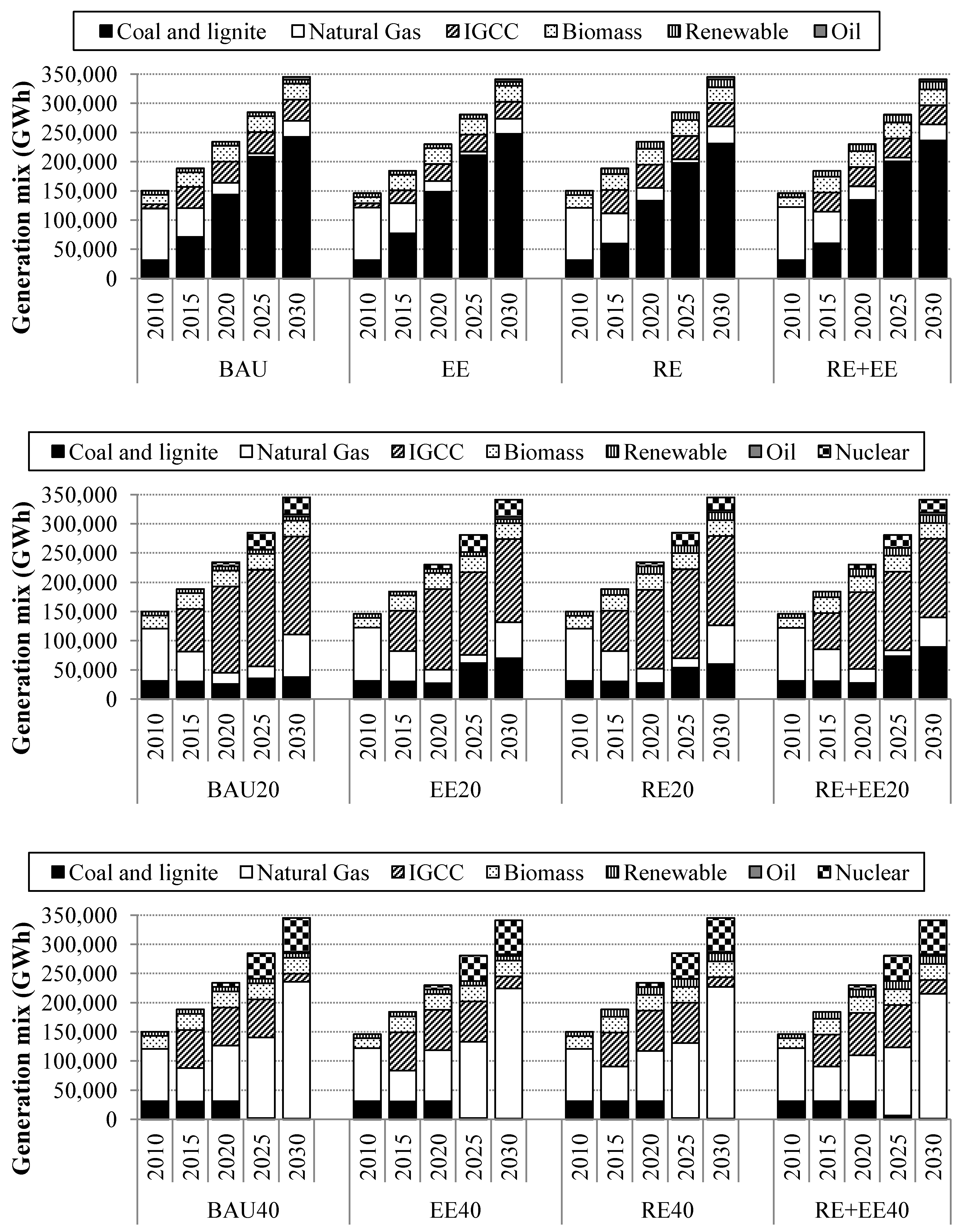
In the BAU scenario coal-fired generating technologies are the largest contributors in electricity generation, as shown in
Figure 2. TH-Coal and IGCC plants would be selected up to 21,717 MW and 17,000 MW by 2030, and would account for 23.6% and 39.3% of power generation in the planning horizon, respectively. The CC-Gas plants, which dominated the power generation share in 2010, would decrease from 57.9% in 2010 down to 5.9% in 2030 due to the retirement of 14,207 MW. It is noted that CC-Gas and GT-Diesel plants are less attractive options than TH-Coal plants in the least cost category due to their high fuel prices. Nonetheless, since capital cost of 800 MW of TH-Coal and 500 MW of IGCC plants is not attractive in the short-term planning because the time needed for breaking even is more, CC-Gas plants of 6000 MW and GT-Diesel plants of 4400 MW are selected at the end of planning period. Additionally, nuclear and renewable energy-based plants are not attractive due to their high capital costs. Nuclear power plant of only 1000 MW would be invested in the year 2020 and only the existing hydro power plants have provided about 6900 GWh per year. Biomass-based technologies play an important role in total generation and cost savings as well as CO
2 emission mitigation. Biomass power is projected to expand to 4100 MW regarding the maximum biomass availability for all scenarios. In the EE, RE and RE+EE scenarios, configurations of capacity and generation mixes are significantly identical to those of the BAU scenario. Under subsidy of adders in the RE and RE+EE scenarios, wind and MSW plants are competitive in comparison to conventional generating technologies. In 2020, wind and MSW plants will be selected at total capacities of 1600 and 400 MW, respectively.
The power generating technologies will shift from conventional coal-fired plants to cleaner technologies when CO
2 emissions are limited. In the BAU20 scenario, IGCC capacity will increase to 19,500 MW, and share about 40.8% of total electricity generation in 2030. The requirement of TH-Coal power plant in BAU scenario would be replaced by CC-Gas plant which would share 23% of power generation in the planning horizon. In addition, 9000 MW nuclear plants will be selected and share about 18.8% of total electricity generation in 2030. Results of the BAU20, EE20, RE20 and RE + EE20 scenarios for CO
2 limitations of 20% lead to the conclusion that TH-Coal, GT-Diesel and renewable energy plants are not competitive in the least cost planning concept (see
Figure 2).
In the BAU40, EE40, RE40 and RE+EE40 scenarios, lower-carbon-content fossil-based technology such as CC-Gas plant is significantly promoted to achieve more CO2 emission reduction. Power generation by IGCC plants in the BAU20 scenario would reduce from 2218 to 606 TWh (by 72.6%) in the BAU40 scenario. Thus CC-Gas plants would contribute 31,200 MW of additional capacity, and share about 2863 TWh of total electricity generation. Increasing CO2 reduction target, from 20% to 40%, results in more renewable energy adoption. Biogas-based plants would be competitive in reduction of substantial CO2 emissions. The biogas-based capacity is expected to be 190 MW in 2030 with respect to the maximum potential.
Figure 2.
Generation mixes in all scenarios.
Figure 2.
Generation mixes in all scenarios.
4.2. CO2 Emission Trends and CO2 Intensity
In the BAU scenario CO
2 emissions have steadily increased due to high coal-based power generation (see
Figure 2). CO
2 emissions in other scenarios without reduction targets are approximately 246-261 Mt-CO
2 in 2030. The average increasing rate of CO
2 emissions for all scenarios is 5.98% per year. It implies that energy savings from efficiency improvement of the NECP have less effect on the traditional demand. The renewable energy in the AEDP plan shares only small proportion when compared to the coal-based plants which result in increasing CO
2 emissions. The government subsidy seems to be insufficient to promote renewable energy technologies, and the power market would still be dominated by fossil-based technologies.
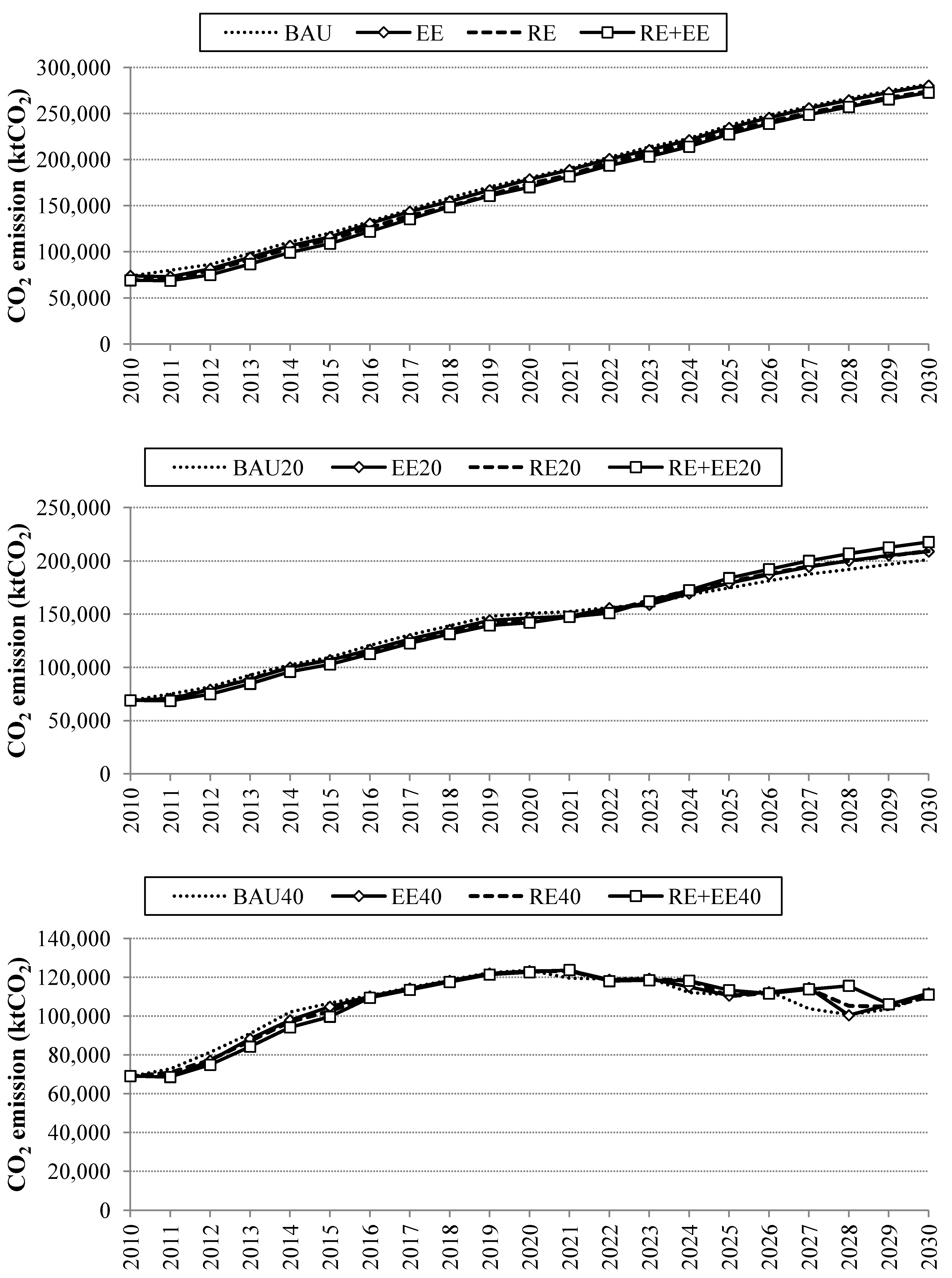
Trends of CO
2 emissions in all CO
2 limitation scenarios are shown in
Figure 3. In the BAU20 scenario, the cumulative emission reduction when compared to the BAU scenario would be 40 and 653 Mt-CO
2 during 2011–2020 and 2021–2030, respectively. The CO
2 emissions in the BAU20, EE20, RE20 and RE+EE20 scenarios have gradually increased, but less than that in the BAU scenario. It is noted that substitution of nuclear power and IGCC plants for coal-based plants will significantly contribute to CO
2 emission reduction.
In the BAU40, EE40, RE40 and RE+EE40 scenarios, electricity production would be dominated by CC-gas, IGCC and nuclear plants with the absence of TH-Coal plants after 2020 (see
Figure 2). As a consequence, the CO
2 emissions of 108 Mt-CO
2 in 2020 would stop increasing and start decreasing. It can be noticed that CO
2 emission would increase again during 2027-2030 because nuclear power plant capacity is limited. In this period, the electricity demand growth would be mainly served by CC-Gas plants which result in increasing CO
2 emissions.
As presented in
Table 6, a significant amount of CO
2 mitigation would be achieved by implementation of the NECP and the AEDP plans. It is noted that electricity demand reduction obtained from energy efficiency improvement in the EE scenario results in 111 Mt-CO
2 of cumulative CO
2 emission reduction when compared to the BAU scenario. In the RE scenario, establishment of renewable energy targets and incorporating adders into the power market mechanism would contribute to CO
2 reduction of 3.12%. Finally, integration of both RE or AEDP and EE or NECP plans will result in environmental benefits. It is proved that 240 Mt-CO
2 of cumulative CO
2 reduction can be achieved in the RE+EE scenario.
In this study, based on historical data of population and Gross Domestic Product (GDP) obtained from the Office of National Economic and Social Development Board of Thailand [
16], average annual population and GDP growths were projected to increase at 0.48% and 4.11%, respectively. In 2009, CO
2 emissions per GDP and
per capita in the power sector were 0.41 kg-CO
2/$US$ and 1.12 t-CO
2, respectively [
17]. In the BAU scenario, CO
2 emissions would increase by 110% in 2030. Nonetheless, the CO
2 emissions per GDP would decrease by 17.6%. Carbon intensity would be significantly improved by application of CO
2 emission constraints. It is noticed that 40% emission reduction would maintain the carbon intensity at 1.41 t-CO
2 per capita. Furthermore, according to [
6], Thailand would import 10,982 MW of power from neighboring countries, and the expected average emission factor will be 0.45 kg-CO
2/kWh.
Table 6 demonstrates that the proposed PGEP plan with 40% CO
2 reduction is able to achieve the expected emission level without power import dependence.
Table 6.
Present worth of total cost, CO2 emissions and fuel import requirement.
Table 6.
Present worth of total cost, CO2 emissions and fuel import requirement.
| Scenario | CO2 emission | Present worth of total cost | Present worth of total cost with subsidy | Incremental abatement cost ($/tCO2) | Fuel imports |
|---|
| (MtCO2) | (kgCO2/kWh) | (tCO2 per capita) | (kgCO2 per GDP) | Billion USD$ | Coal (Mt) | Natural gas (MM.scf/day) | Vulnerability (% to GDP) |
|---|
| BAU | 3824 | 0.73 | 2.58 | 0.38 | 132.90 | - | - | 1167 | - | 1.17% |
| EE | 3766 | 0.72 | 2.54 | 0.38 | 131.12 | - | −27.00 | 1142 | - | 1.14% |
| RE | 3673 | 0.70 | 2.48 | 0.37 | 135.45 | 132.31 | 18.38 | 1101 | - | 1.10% |
| RE+EE | 3616 | 0.69 | 2.44 | 0.36 | 133.69 | 130.59 | 5.70 | 1077 | - | 1.08% |
| BAU20 | 3059 | 0.59 | 2.06 | 0.31 | 136.13 | - | 2.24 | 848 | - | 0.85% |
| EE20 | 133.30 | - | −0.20 | 852 | - | 0.85% |
| RE20 | 137.76 | 134.26 | 5.49 | 846 | - | 0.85% |
| RE+EE20 | 135.03 | 131.77 | 3.01 | 854 | - | 0.86% |
| BAU40 | 2295 | 0.44 | 1.55 | 0.23 | 152.09 | - | 7.08 | 351 | 847 | 1.00% |
| EE40 | 148.47 | - | 5.26 | 373 | 709 | 0.92% |
| RE40 | 153.12 | 149.09 | 8.20 | 373 | 686 | 0.90% |
| RE+EE40 | 149.49 | 145.64 | 6.35 | 395 | 553 | 0.82% |
Figure 3.
Trends of CO2 emissions in the CO2 limitation scenarios.
Figure 3.
Trends of CO2 emissions in the CO2 limitation scenarios.
4.3. Present Worth of Total Cost and Incremental Abatement Cost
In the EE scenario, 1.34% of present worth of total cost can be saved when compared to the BAU scenario due to the implementation of the NECP plan (see
Table 6). Because of high capital cost of renewable energy technologies, renewable subsidy and development targets in the AEDP lead to increasing the total cost by 1.9% in comparison to the BAU scenario. In addition, when both plans are integrated, the total cost of RE+EE scenario is higher than the BAU scenario. The costs in the CO
2 limitation scenarios are higher due to more investment in cleaner generating technologies. For the CO
2 emission reduction of 40%, the costs in 2030 will increase by 14.4%, 11.7%, 15.2% and 12.4% when compared to the corresponding BAU, EE, RE, and RE+EE scenarios, respectively. Furthermore, the 20% CO
2 reduction scenarios would require much lower incremental cost, a reduction of 1.85% on average.
In this study, the incremental abatement cost (IAC) represents the proportion of the incremental cost to CO2 emission reduction when compared to the BAU scenario. The EE scenario show negative IACs due to savings achieved by energy efficiency measures in the NECP plan. In the RE scenario, the power expansion targets and subsidies of adders in the AEDP plan result in the highest IAC of 23.42 US$/t-CO2. It is noted that the IACs in the EE20 and RE20 scenarios are relatively small. Nonetheless, the IACs are higher in range between 11.15 and 14.48 US$/t-CO2 in the EE40 and RE40 scenarios.
4.4. Fuel Import Vulnerability
The electricity production in all scenarios employs both coal-fired and gas-fired generating technologies. Nonetheless, indigenous coal resources are not enough to meet the power demand and coal mining has encountered the public opposition. Furthermore, Thailand produced 30,880 million m
3 of natural gas in 2011 and has proven reserves of 312,200 million m
3 [
18]. Thus the need for imported coal and natural gas result in less energy supply security. In this study the indigenous natural gas of 310,000 million m
3 is presumed to be available for the PGEP according to the proven reserves during 2011–2030. Therefore, the imported gas is taken into account when the excessive natural gas supply is required.
The coal import requirement of 1,049 Mt in the BAU scenario is abated by 31.3% and 77.9% in the BAU20 and BAU40 scenarios, respectively (see
Table 6). The fuel import vulnerability in Thailand’s power system is represented by the proportion of total imported fuel cost to the total GDP [
8]. It can be seen that the import vulnerability of the BAU40 scenario will deteriorate by 5.68% compared to the BAU scenario due to more natural gas import. As a co-benefit of CO
2 emission reduction, both imported coal and gas in the BAU20 scenario decrease resulting in vulnerability improvement of 31.3%. It is noted that CO
2 emission limitation, energy efficiency improvement, renewable power generation as well as adders not only mitigate substantial CO
2 emissions but also reduce imported fuel dependency.
4.5. Sensitivity Analysis
Parameter setting in the PGEP model may cause dramatic changes in the results. In this study, two important parameters which are discount rate and escalation rate of fuel prices have been taken into account for sensitivity analysis. Both parameters have been considered in two other rates: 5% and 10% for discount rate, and 2.3% and 4% per year for escalation rate. Four different cases under these rates (herein referred to as BAU-E2D10, BAU-E2D5, BAU-E4D10 and BAU-E4D5) were composed for comparative assessment. For the sake of completeness it should be mentioned that the reference case is officially the BAU-E2D10 case in the forthcoming explanation.
The prefix “BAU” is changed to “20%CO2” and “40%CO2” when 20% and 40% of CO2 emission reduction targets are applied to the PGEP model. The 10% of discount rate and 2.3% of escalation rate, which is the reference case in this analysis, provide comparative details in terms of generation mix, CO2 emission, the present worth of total cost and vulnerability, as shown in the previous sub-section. Hence, the 20%CO2-E2D10 and 40%CO2-E2D10 are also reference cases.
From
Table 7, it can be noticed that capital intensive generating technologies would be augmented more than those of the reference case due to increasing fuel price and decreasing discount rate. Nuclear power plant in the BAU-E2D5, BAU-E4D10 and BAU-E4D5 cases would provide more power generation by 245%, 364% and 490%, respectively. For achieving 20% and 40% reduction targets, both parameters (escalation rate and discount rate) do not influence the selection of nuclear power plant, which was selected only up to its maximum capacity in the reference cases (20% CO-E2D10 and 40% CO-E2D10).
Likewise it should be noted that the coal and lignite utilization in the power sector is decreasing which can be attributed to the increase of IGCC in the generation mix and this is in comparison to the BAU in all the other cases with parametric changes. But in the case of BAU with reduction target, natural gas utilization increases and IGCC capacity decreases which might seem counter-intuitive. The reason for this is that the model makes an economic compromise between the targeted reduction of CO2 emissions and the escalation of fuel prices, and then it selects the least cost technology which happens to be natural gas technology.
Although renewable energy would not be selected as much as the nuclear power in the BAU-E2D5, BAU-E4D10 and BAU-E4D5 cases because of their capital intensiveness and low capacity factor, they would play an important role in reducing CO2 emission with high fuel price and low discount rate. Renewable energy would account for 5.5% of total power generation in the 20% CO2-E4D5 case which is more than that in the corresponding reference case (20% CO2-E2D10) by 2%.
As reported in
Table 8, decreasing discount rate by 5% from the reference case (BAU-E2D10) would increase the present worth of total cost by 52.2% in the BAU-E2D5 case. The cost would increase by only 9.1% in the BAU-E4D10 case when the escalation rate of 4% per year is applied. Nonetheless, the CO
2 emission from the BAU-E4D10 case would decrease by 9.6% when compared to the reference case (BAU-E2D10), whilst decreasing by 6.8% in the BAU-E2D5 case. Thus, when 20% and 40% of CO
2 emission reduction targets are taken into account, the incremental abatement cost would be substantially high due to increase in the generation and expansion cost. The 20% CO
2-E4D5 and 40% CO
2-E4D5 would require higher abatement cost than both corresponding reference cases (20% CO
2-E2D10 and 40% CO
2-E2D10), by 785% and 295% respectively. In terms of vulnerability of the power sector the paper presents the fuel import vulnerability for the various scenarios. The significant aspect to be noted is that when the reduction target increases to 40% the vulnerability increases, albeit by a small margin. The reason for this is two-fold. One is the escalation in the fuel prices and the other is the increase in the natural gas usage in the generation mix which has a much higher price than that of coal. These two reasons combined increase the fuel import vulnerability of the power sector. Hence this analysis proves that whilst having reduction targets is mandatory if CO
2 emissions are to be reduced this should be done in tandem with policies which compulsorily implement renewable technologies. Another aspect to be noted is that for a marginal increase in vulnerability a country possessing a power sector like Thailand may implement reduction targets which in turn reduce the utilization of coal and lignite.
Table 7.
Comparative generation mix for the sensitivity analysis.
Table 7.
Comparative generation mix for the sensitivity analysis.
| Fuel type | BAU-E2D10 (Reference case) | BAU-E2D5 | BAU-E4D10 | BAU-E4D5 |
|---|
| Electricity production for entire planning horizon (TWh) |
|---|
| Coal and lignite | 1575 | 1001 | 950 | 753 |
| Natural Gas | 745 | 722 | 723 | 708 |
| IGCC | 2052 | 2481 | 2415 | 2609 |
| Biomass | 551 | 522 | 547 | 522 |
| Renewable | 152 | 153 | 152 | 158 |
| Oil | 6 | 6 | 3 | 2 |
| Nuclear | 80 | 276 | 371 | 407 |
| Other | 56 | 56 | 56 | 56 |
| Fuel type | 20%CO2-E2D10 (Reference case) | 20%CO2-E2D5 | 20%CO2-E4D10 | 20%CO2-E4D5 |
| Electricity production for entire planning horizon (TWh) |
| Coal and lignite | 533 | 426 | 442 | 298 |
| Natural Gas | 1198 | 1428 | 1658 | 1589 |
| IGCC | 2218 | 1991 | 1754 | 1933 |
| Biomass | 579 | 579 | 579 | 579 |
| Renewable | 171 | 275 | 254 | 287 |
| Oil | 3 | 2 | 1 | 2 |
| Nuclear | 458 | 458 | 473 | 473 |
| Other | 56 | 56 | 56 | 56 |
| Fuel type | 40%CO2-E2D10 (Reference case) | 40%CO2-E2D5 | 40%CO2-E4D10 | 40%CO2-E4D5 |
| Electricity production for entire planning horizon (TWh) |
| Coal and lignite | 411 | 327 | 373 | 212 |
| Natural Gas | 2864 | 3102 | 3283 | 3209 |
| IGCC | 607 | 404 | 174 | 396 |
| Biomass | 579 | 579 | 579 | 579 |
| Renewable | 239 | 288 | 277 | 290 |
| Oil | 3 | 2 | 1 | 2 |
| Nuclear | 458 | 458 | 473 | 473 |
| Other | 56 | 56 | 56 | 56 |
Table 8.
Economic and environmental results of the sensitivity analysis.
Table 8.
Economic and environmental results of the sensitivity analysis.
| Scenario | Escalation rate | Discount rate | CO2 emission reduction target | CO2 emission | Present worth of total cost | Incremental abatement cost | Fuel import vulnerability (% to GDP) |
|---|
| (MtCO2) | (kgCO2/kWh) | Billion USD$ | ($/tCO2) |
|---|
| BAU-E2D10 | 2.3 | 10 | - | 3489 | 0.67 | 132.90 | - | 1.05% |
| BAU-E2D5 | 5 | 3252 | 0.62 | 202.28 | 0.97% |
| BAU-E4D10 | 4 | 10 | 3154 | 0.60 | 145.01 | 0.93% |
| BAU-E4D5 | 5 | 3104 | 0.59 | 224.96 | 0.91% |
| 20%CO2-E2D10 | 2.3 | 10 | 20% | 2792 | 0.54 | 136.13 | 4.62 | 0.72% |
| 20%CO2-E2D5 | 5 | 2602 | 0.50 | 217.10 | 22.78 | 0.63% |
| 20%CO2-E4D10 | 4 | 10 | 2523 | 0.48 | 156.01 | 17.44 | 0.63% |
| 20%CO2-E4D5 | 5 | 2483 | 0.48 | 250.36 | 40.92 | 0.61% |
| 40%CO2-E2D10 | 2.3 | 10 | 40% | 2094 | 0.40 | 152.09 | 13.75 | 1.11% |
| 40%CO2-E2D5 | 5 | 1951 | 0.37 | 249.75 | 36.49 | 1.17% |
| 40%CO2-E4D10 | 4 | 10 | 1892 | 0.36 | 177.27 | 25.58 | 1.25% |
| 40%CO2-E4D5 | 5 | 1862 | 0.36 | 292.36 | 54.29 | 1.23% |
4.6. Model Uncertainty and Policy Implication
The results presented, whilst being significant in understanding the implications of EE and RE on the power sector of Thailand, do need to be read with certain caveats. The inherent weakness of the model is that it is a single objective optimization model. Once all the constraints have been satisfied the model will select the cheapest generating technology. The extraneous aspects which contribute to the uncertainty of the model are multi-fold. The model does not accommodate sudden and unexpected changes in fuel or technology prices. This may lead to the actual situation being significantly different to the model results. Another aspect is that the model cannot depict the inherent inertia of a very large power system.
However, the policy measures modeled in this study prove the necessity of EE and RE to Thailand but it is important that policy makers also understand the implications and barriers. In the case of nuclear power plant the public perception may need to be improved before any attempt is made to commissioning. Another important aspect for policy makers are measures to alleviate institutional barriers regarding RE technologies and the support of continuous improvement in the EE measures which would need cooperation from stakeholders.
5. Conclusions
In this study, the optimal PGEP plans with regard to CO2 mitigation and selected government policies on RE and EE are provided in order to analyze generation mix, CO2 intensity, cost savings, mitigation costs as well as imported fuel requirement. Results indicate that traditional coal-based plants dominate in PGEP in terms of generation cost resulting in high CO2 intensity. The power generation from IGCC and nuclear plants must increase in order to achieve the 20% CO2 reduction target. In addition to increasing nuclear power utilization, natural gas resource will play an important role in power generation in regard to the 40% CO2 reduction target.
The energy efficiency improvement and adders as well as increasing renewable energy utilization will contribute to large CO2 mitigation in the power sector. In addition, the NECP and AEDP also provide co-benefits in terms of decreasing imported fuel vulnerability. The abatement costs of the 40% CO2 reduction scenarios range from 5.26 to 8.20 US$/tCO2, which are significantly higher than the 20% CO2 reduction scenarios scenario. The CO2 emission reduction definitely provides the satisfaction of government-expected average emission of 0.44 kg-CO2/kWh without power import requirement.

