A Fuzzy Group Forecasting Model Based on Least Squares Support Vector Machine (LS-SVM) for Short-Term Wind Power

Abstract

Many models have been developed to forecast wind farm power output. It is generally difficult to determine whether the performance of one model is consistently better than that of another model under all circumstances. Motivated by this finding, we aimed to integrate groups of models into an aggregated model using fuzzy theory to obtain further performance improvements. First, three groups of least squares support vector machine (LS-SVM) forecasting models were developed: univariate LS-SVM models, hybrid models using auto-regressive moving average (ARIMA) and LS-SVM and multivariate LS-SVM models. Each group of models is selected by a decorrelation maximisation method, and the remaining models can be regarded as experts in forecasting. Next, fuzzy aggregation and a defuzzification procedure are used to combine all of these forecasting results into the final forecast. For sample randomization, we statistically compare models. Results show that this group-forecasting model performs well in terms of accuracy and consistency.

1. Introduction

Along with science and technology in general, wind power technology has also developed rapidly. Because wind power technology is mature, many medium- and large-sized wind farms have been built and put into operation. Wind power has become an important source of the entire power system; worldwide, the installed wind power capacity was 157.9 GW in 2009, representing an annual growth of 20% over the preceding 10 years. Wind energy resources available in China are estimated at 1000 GW, ranking the country third after Russia and the U.S. In recent years, wind power has experienced rapid development in China, as the capacity increased from 0.34 to 25.8 GW between 2000 and 2009. In 2020, the total installed capacity of wind power is expected to reach 150 GW [1].

Wind power is always fluctuating because wind is volatile and intermittent. When the power output exceeds a certain value, it significantly affects power quality, power system security and the stability of operations. If an accurate short-term wind power output forecast is available, the power dispatching department can adjust scheduling in accordance with changes in wind power output to ensure power quality and reduce the system’s excess capacity and power system cost. Therefore, short-term wind power forecasts are of key importance [2,3,4].

Modern wind farms usually incorporate remote monitoring systems in wind turbines so that all turbines can capture and record all signals. The real-time output data from wind generators can be used directly for wind power forecasts without any additional cost, which reduces the cost and improves the quality of data collection, as well as increases forecast accuracy. The existing forecasting methods can be classified into two groups. The first group consists of univariate forecasting models based on historical and real-time power data, in which changes in wind speed are not considered. The second group consists of multivariate models, in which forecasts are based on the relationship between weather data and output power [5]. The numerical weather prediction (NWP) model is popular for short-term wind power prediction with advantages in accuracy, but, it needs more weather information [6]. Detailed algorithms include time series methods, such as the auto-regressive moving average (ARMA) and the auto-regressive conditional heteroskedasticity (ARCH) models [7,8], the linear regression model [9], the grey theory model [10,11], the support vector machine (SVM) [12,13], adaptive fuzzy logic algorithms [14,15] and artificial neural networks (ANNs) [16,17], among others [18].

In the above-mentioned individual models, it is difficult to determine whether the performance of one model is consistently better than that of another model under all circumstances. Typically, a number of different models are utilised, and the model with the most accurate results is selected. However, the selected model may not necessarily be the best for future use because of potentially influential factors, such as sampling variation, model uncertainty and structure change. It is almost universally agreed upon in the forecasting literature that no single method is best in every situation, primarily because a real-world problem is often complex in nature and because any single model may not be able to capture different patterns equally well. Therefore, there is a certain optimal combination of forecasts to be studied, such as an adaptive combination of forecasts [19] and an optimal combination of wind power forecasts [20]. Motivated by this finding, we aimed to integrate multiple models into an aggregated model to obtain further performance improvement. Therefore, certain intelligent SVM forecasting models were developed. The models are selected by a decorrelation maximisation method, and the remaining models can be regarded as experts in forecasting. Then, the fuzzy theory is used to combine all of these forecasting results into the final forecast.

The remainder of this paper is organised as follows: Section 2 describes three group models. In Section 3, real datasets are statistically used for the testing of these models. Finally, conclusions are presented in Section 4.

2. The Forecasting Model

2.1. Principle of Least Squares SVM (LS-SVM)

In this study, SVM was selected as the basic algorithm with which to construct forecasting models because this algorithm is often viewed as a “universal approximator”. It has been proven to provide a good arbitrary approximation of any continuous function. Therefore, the model is used here to simulate mutual relationships between historical data and the forecast power output. The models have the ability to provide flexible mapping between inputs and outputs. The SVM model of a data set is given by the formula described below.

Consider an n set of data{(x₁, y₁), …, (x_N, y_N)}, where x_i is the i_th input vector and y_i is the corresponding desired output. Because i = 1, 2, …, N, where N is the size of the sample, the estimating function assumes the following form:

$$f(x)=w\cdot \varphi (x)+b$$

(1)

where w is the weight vector, b is the bias and ϕ(x) is the high-dimensional feature space nonlinearly mapped from the input space, and (·) represents the inner product.

This leads to the optimisation problem associated with standard SVM:

$$\min R_{str}=\frac{1}{2}{\Vert w\Vert }^2+\gamma R_{emp}$$

(2)

where γ is a positive real constant that determines the penalty for estimation errors and $R_{emp}(w,b)=\frac{1}{N}{\displaystyle \sum _{i=1}^N{\left|y_i-f(x_i)\right|}_{\delta }}$ is the estimation error measured by the experimental risk and loss function. Usually, the ε- insensitive loss function is adopted because of its excellent sparsity:

(3)

For least-squares SVM (LS-SVM), the two norms of the estimation error are adopted as the loss function in the objective function and equality constraints instead of inequality constraints. Therefore, the optimisation problem is described as:

(4)

where ξ_i is a slack variable, ξ_i ≥ 0. It is a variable added to an inequality constraint to transform it to equality. It is non-negative number in this paper.

After the introduction of Lagrange multipliers α_i, the Lagrange function is constructed as:

(5)

According to KKT conditions which can transform inequality constraints into equality constraints, defined as:

(6)

The following equation can then be obtained:

(7)

After eliminating w and γ, we obtain:

(8)

where Θ = [1, …, 1]_1×N, I is a unit matrix, Ω is a square matrix and the element of Ω is expressed as: Ω_ij = ϕ(x_i)^T ϕ(x_j). In the equation (8), α = [α₁, …, α_N], y = [y₁, …, y_N].

By solving Equation (7), values of α and b are obtained. According to Mercer's condition, there exists a kernel function with a value that is equal to the inner product of the two vectors x_i and x_j in the feature spaces ϕ(x_i) and ϕ(x_j); that is, K(x_i, x_j) = ϕ(x_i)^T ϕ(x_j). Then, the LS-SVM model for regression is expressed as:

$$y(x)={\displaystyle \sum _{i=1}^N{\alpha }_i}K(x,x_i)+b$$

(9)

2.2. Group Model Based on LS-SVM

2.2.1. Group 1: Diversified Univariate LS-SVM Model

The first group is the univariate forecasting model. It is based on historical and real-time power data; other weather data, such as wind speed, are not considered. Many experimental results have shown that the generalisation of individual networks is not unique. Even for some simple problems, different SVMs with different settings (e.g., different network architectures and different initial conditions) may result in different generalisation results. Diverse models are generated by selecting different core learning algorithms, such as the steep-descent algorithm, the Levenberg-Marquardt algorithm and other training algorithms [21]. Finally, 10 different univariate least squares support vector machine (LS-SVM) models are formulated [22,23]. All of these models use the Gaussian function as the kernel function, and the output is the one-hour-ahead forecasted wind power output. Other parameters are shown in Table 1.

Table 1. Ten univariate LS-SVM models.

Models	Inputs	γ	σ2
LS-SVM-1	3 previous observations	10	5
LS-SVM-2	4 previous observations	20	5
LS-SVM-3	5 previous observations	30	5
LS-SVM-4	6 previous observations	40	5
LS-SVM-5	7 previous observations	50	5
LS-SVM-6	3 previous observations	50	2
LS-SVM-7	4 previous observations	50	4
LS-SVM-8	5 previous observations	50	6
LS-SVM-9	6 previous observations	50	8
LS-SVM-10	7 previous observations	50	10

Table 1. Ten univariate LS-SVM models.

Models	Inputs	γ	σ2
LS-SVM-1	3 previous observations	10	5
LS-SVM-2	4 previous observations	20	5
LS-SVM-3	5 previous observations	30	5
LS-SVM-4	6 previous observations	40	5
LS-SVM-5	7 previous observations	50	5
LS-SVM-6	3 previous observations	50	2
LS-SVM-7	4 previous observations	50	4
LS-SVM-8	5 previous observations	50	6
LS-SVM-9	6 previous observations	50	8
LS-SVM-10	7 previous observations	50	10

2.2.2. Group 2: Diversified Univariate Hybrid Model of ARIMA and the SVM Model

2.2.2.1. Brief Introduction of the Hybrid Model

Because real-world time series are rarely purely linear or nonlinear, researchers have revealed that hybrid models that hybridise two or more different algorithms can produce forecasts of higher accuracy than those produced by individual models. ARIMA and LS-SVM models have different capabilities of capturing data characteristics in linear and nonlinear domains; therefore, the hybrid model proposed in this study is composed of an ARIMA component and an LS-SVM component. Thus, the hybrid model is expected to capture linear and nonlinear patterns with improved overall forecasting performance. Experimental results with real data sets indicate that the hybrid model can be an effective means by which to improve forecasting accuracy over that achieved by either of the models separately. In this section, a type of hybrid approach using both ARIMA and LS-SVM models is proposed. Because ARIMA is a linear model [24] and LS-SVM [22,25] is a nonlinear model, the hybrid approach is expected to capture both linear and nonlinear patterns in wind park power time series.

Based on the structure proposed by [26], the hybrid model (y_t) can be represented as:

$$y_t=L_t+N_t$$

(10)

where L_t denotes the linear component and N_t denotes the nonlinear component.

These two components must be estimated from the data. First, ARIMA is used to model the linear component, resulting in the residuals from the linear model containing only the nonlinear relationship. The residual at time t (from the linear model) is denoted as e_t, and then:

$$e_t=y_t-{\widehat{L}}_t$$

(11)

where ${\widehat{L}}_t$ is the forecast value at time t from the ARIMA models. Specifications of the (1, 0, 0) × (0, 1, 1) model are as described in Equation (11):

$$Y_t=\delta +Y_{T-4}+{\varphi }_1(Y_{t-1}-Y_{t-5})$$

(12)

Residuals are also important. By modelling residuals using LS-SVM, nonlinear relationships can be discovered. With n input nodes, the LS-SVM model for residuals will be:

$$e_t=f(e_{t-1},e_{t-2},\dots e_{t-n})+{\Delta }_t$$

(13)

where f is a nonlinear function determined by the LS-SVM model and Δ_t is its corresponding random error. Therefore, the forecast of the hybrid model is:

$${\widehat{y}}_t={\widehat{L}}_t+{\widehat{e}}_t$$

(14)

2.2.2.2. Generating the Diversified Hybrid Model from the ARIMA and LS-SVM Models

The proposed hybrid method is applied to forecast wind power output, i.e., the LS-SVM model is used to model the nonlinearity of residuals obtained from the ARIMA models. As mentioned in Section 2.1, to generate the diverse models, the structure of the above LS-SVM can be varied by changing the number of nodes in the input layer and the second layer. Because the number of input layers is changed, there should be different training data. These data can be acquired by re-sampling and pre-processing the data. There are many techniques that can be used to obtain diverse training data sets, such as bagging noise injection, cross-validation and stacking. With these different training datasets and structures, 10 diverse hybrid models are generated using ARIMA and LS-SVM models as described in Table 2. For all of these models, the linear parts use ARIMA (Y_t = δ + Y_T−4 + ϕ₁(Y_t−1 − Y_t−5) and the nonlinear parts use different LS-SVMs. All of these LS-SVM models use the Gaussian function as the kernel function, and the output is the forecasted error. Other parameters are shown in Table 2.

Table 2. Ten diverse hybrid models using ARIMA and LS-SVM.

Models	Inputs	γ	σ2
H-AR-LS-1	3 previous observations	10	5
H-AR-LS-2	4 previous observations	20	5
H-AR-LS-3	5 previous observations	30	5
H-AR-LS-4	6 previous observations	40	5
H-AR-LS-5	7 previous observations	50	5
H-AR-LS-6	3 previous observations	50	2
H-AR-LS-7	4 previous observations	50	4
H-AR-LS-8	5 previous observations	50	6
H-AR-LS-9	6 previous observations	50	8
H-AR-LS10	7 previous observations	50	10

Table 2. Ten diverse hybrid models using ARIMA and LS-SVM.

Models	Inputs	γ	σ2
H-AR-LS-1	3 previous observations	10	5
H-AR-LS-2	4 previous observations	20	5
H-AR-LS-3	5 previous observations	30	5
H-AR-LS-4	6 previous observations	40	5
H-AR-LS-5	7 previous observations	50	5
H-AR-LS-6	3 previous observations	50	2
H-AR-LS-7	4 previous observations	50	4
H-AR-LS-8	5 previous observations	50	6
H-AR-LS-9	6 previous observations	50	8
H-AR-LS10	7 previous observations	50	10

2.2.3. Group 3: Diversified Multivariate LS-SVM model

In this group of multivariate methods, the relationship between weather data and power output is considered. There are five fundamental variables that impact wind power output. The first, w₁, is the wind speed, measured in metres/second (m/s); the second, w₂, is the wind direction, measured as the angle between the incoming wind and the north; the third, w₃, is the air temperature, measured in °C; the fourth, w₄, is the atmospheric pressure in Pa; and the fifth, w₃a, is the relative humidity. These five fundamental variables are used as input data, and the wind power output is the output of the LS-SVM model.

To generate the diverse models, the structure of the above LS-SVM model is varied by changing the number of nodes in the second layer. Different initial conditions can also create diversity in models; these initial conditions include random weights, learning rates and momentum rates from which each network is trained. With these different initial conditions and structures, 10 diverse LS-SVMs are generated. All of these models use the Gaussian function as the kernel function, and the output is the one-hour-ahead forecasted wind power output. Other parameters are shown in Table 3.

Table 3. Ten diverse multivariate LS-SVMs.

Models	Inputs	γ	σ2
DLS-SVM-1	w1; w2; w3; w3; w4; w5; 2 previous observations	10	5
DLS-SVM-2	w1; w2; w3; w3; w4; w5; 2 previous observations	20	5
DLS-SVM-3	w1; w2; w3; w3; w4; w5; 2 previous observations	30	5
DLS-SVM-4	w1; w2; w3; w3; w4; w5; 2 previous observations	40	5
DLS-SVM-5	w1; w2; w3; w3; w4; w5; 2 previous observations	50	5
DLS-SVM-6	w1; w2; w3; w3; w4; w5; 3 previous observations	50	2
DLS-SVM-7	w1; w2; w3; w3; w4; w5; 3 previous observations	50	4
DLS-SVM-8	w1; w2; w3; w3; w4; w5; 3 previous observations	50	6
DLS-SVM-9	w1; w2; w3; w3; w4; w5; 3 previous observations	50	8
DLS-SVM-10	w1; w2; w3; w3; w4; w5; 3 previous observations	50	10

Table 3. Ten diverse multivariate LS-SVMs.

Models	Inputs	γ	σ2
DLS-SVM-1	w1; w2; w3; w3; w4; w5; 2 previous observations	10	5
DLS-SVM-2	w1; w2; w3; w3; w4; w5; 2 previous observations	20	5
DLS-SVM-3	w1; w2; w3; w3; w4; w5; 2 previous observations	30	5
DLS-SVM-4	w1; w2; w3; w3; w4; w5; 2 previous observations	40	5
DLS-SVM-5	w1; w2; w3; w3; w4; w5; 2 previous observations	50	5
DLS-SVM-6	w1; w2; w3; w3; w4; w5; 3 previous observations	50	2
DLS-SVM-7	w1; w2; w3; w3; w4; w5; 3 previous observations	50	4
DLS-SVM-8	w1; w2; w3; w3; w4; w5; 3 previous observations	50	6
DLS-SVM-9	w1; w2; w3; w3; w4; w5; 3 previous observations	50	8
DLS-SVM-10	w1; w2; w3; w3; w4; w5; 3 previous observations	50	10

2.3. Group Model Based on LS-SVM

As mentioned above, each group consists of 10 forecasting models. We need to select a subset of representatives to improve ensemble efficiency. It is clear that it is a necessary requirement of diverse models for making fuzzy group decisions. In this study, a decorrelation maximisation method was used to select the appropriate number of ensemble members. As noted previously, the basic starting point of the decorrelation maximisation algorithm is the principle of ensemble model diversity; that is, the correlations between the selected models should be as small as possible. If there are p models (f₁, f₂, …, f_p) with n forecast values, an error matrix (e₁, e₂, …, e_p) of p predictors can be represented by:

(15)

From the matrix, the mean, variance and covariance of E can be calculated as:

(16)

(17)

(18)

Considering Equations (17) and (18), we can obtain a variance covariance matrix:

$$V_{p\times p}=(V_{ij})$$

(19)

Based on the variance-covariance matrix, correlation matrix R can be calculated using the following equations:

$$R=(r_{ij})$$

(20)

$$r_{ij}=\frac{V_{ij}}{\sqrt{V_{ii}{V}_{jj}}}$$

(21)

where r_ij is the correlation coefficient, representing the degrees of correlation classifiers f_i and f_j.

Subsequently, the plural-correlation coefficient ρf_i|(f₁, f₂, …, f_i−1, f_i+1, …, f_p) between classifier f_i and other p − 1 classifiers can be computed based on the results of Equations (20) and (21). For convenience, ρf_i|(f₁, f₂, …, f_i−1, f_i+1, …, f_p) is abbreviated as ρ_i, representing the degree of correlation between f_i and (f₁, f₂, …, f_i−1, f_i+1, …, f_p). To calculate the plural-correlation coefficient, the correlation matrix R can be represented by a block matrix; that is:

(22)

where R − i denotes the deleted correlation matrix. It should be noted that r_ii = 1(i = 1, 2, …, p). Next, the plural-correlation coefficient can be calculated by:

$${\rho }_i^2=r_i^T{R}_{-i}^T{r}_i(i=1,2,\dots p)$$

(23)

For a pre-specified threshold θ, if ρ_i² > θ, then model f_i should be removed from p models. Otherwise, model f_i should be retained. Generally, the decorrelation maximisation algorithm can be summarised in the following steps:

Computing the variance-covariance matrix V_ij and the correlation matrix R with Equations (19) and (20). For the i_th classifier (i = 1, 2, …, p), the plural-correlation coefficient ρ_i can be calculated using Equation (23).

For a pre-specified threshold θ, if ρ_i < θ, then the i_th classifier should be deleted from the ρ classifiers. Conversely, if ρ_i > θ, then the i_th classifier should be retained. For each group of models, we select eight as the representative for the subsequent step.

2.4. Fuzzy Group Prediction

For a specified forecasting problem, different experts usually give different estimations based on a set of criteria X = (c₁, c₂, ..., c_m). Some experts give optimistic estimates, some prefer pessimistic estimates, and others present the most likely estimates. To incorporate these different judgements into the final forecasting result and to make full use of the different estimates, a process of fuzzification is used. In this paper, a typical triangular fuzzy number can be used to describe the forecasting results provided by the experts; that is:

$${\tilde{Z}}_i=(z_{i1},z_{i2},z_{i3})=(\text{the lowest forecast value};\text{the most likely forecast value};\text{the highest forecast value}), \text{where} i\text{ represents the numerical index of experts}.$$

Like human experts, individual LS-SVM forecasting groups can also generate different forecasting results by using different parameter settings and training sets. For example, the first forecasting group (univariate LS-SVM model group) generates eight different forecasting results from the eight models (selected from the first 10 models; Section 2.3) of different hidden neurons or different initial weights. The entire first group can be considered an expert in forecasting. Assume that this expert produces k different results, $f_1^i(X_A),f_2^i(X_A),\dots f_k^i(X_A)$, for a specified applicant “A” over a set of models of different hidden neurons or different initial weights in this group. To make full use of all of the information provided by these results, without loss of generalisation, we use the triangular fuzzy number to construct the fuzzy opinion for consistency; that is the smallest, average and largest of the k forecasting results are used as the left-, medium- and right-membership degrees, respectively. In other words, the smallest and largest scores are seen as optimistic and pessimistic evaluations, respectively, and the average forecasting result is considered to be the most likely score. Of course, the median can also be used as the most likely score to construct the triangular fuzzy number. However, that approach can cause the loss of certain useful information because some other scores are ignored. Therefore, the average is selected as the most likely power output to incorporate the full information from all of the models into the fuzzy judgement. Using this fuzzification method, the expert can make a fuzzy forecast for each point. More precisely, the triangular fuzzy number used for forecasting can be represented as:

(24)

Suppose there are p experts, and let ${\tilde{Z}}_i=\psi ({\tilde{Z}}_1,{\tilde{Z}}_2,\dots {\tilde{Z}}_p)$ be the aggregation of p fuzzy judgements, where ψ() is an aggregation function. Many methods have been developed to determine the aggregation function. Usually, fuzzy judgements of the p group members are aggregated by using a common linear additive procedure; that is:

(25)

where w_i is the weight of the i_th fuzzy judgement, i = 1, 2, ..., p. The weights usually satisfy the following normalisation condition:

$${\displaystyle \sum _{i=1}^p{w}_i}=1$$

(26)

At this point, the goal is to determine the optimal weight w_i of the i_th fuzzy expert. In this study, three groups of models are used as experts, and we give them the same weight of 1/3 each. After completing aggregation, a fuzzy group consensus can be obtained using Equation (25). To obtain a crisp value of the credit score, we use a defuzzification procedure to obtain the crisp value for decision-making purposes. According to Bortolan and Degani, the defuzzified value of a triangular fuzzy number ${\tilde{Z}}_i=(z_1,z_2,z_{i3})$ can be determined by its centroid, which is computed by:

(27)

At this point, a final group consensus has been computed using the above process. To summarise, the proposed intelligent-agent-based fuzzy group forecasting model is comprised of five steps:

(1)

Three forecasting groups are presented, and each group has eight models with varied structures and initial data, for example.

(2)

Based on the datasets, each forecasting group can produce eight different forecasting results from the different models.

(3)

For the different forecasting results, Equation (25) is used to fuzzify the judgements of intelligent agents into fuzzy opinions.

(4)

The fuzzy opinions are aggregated into a group consensus, using the optimisation method proposed above, in terms of the maximum agreement principle.

(5)

The aggregated fuzzy group consensus is defuzzified into a crisp value. This defuzzified value can be used as the final forecasting result.

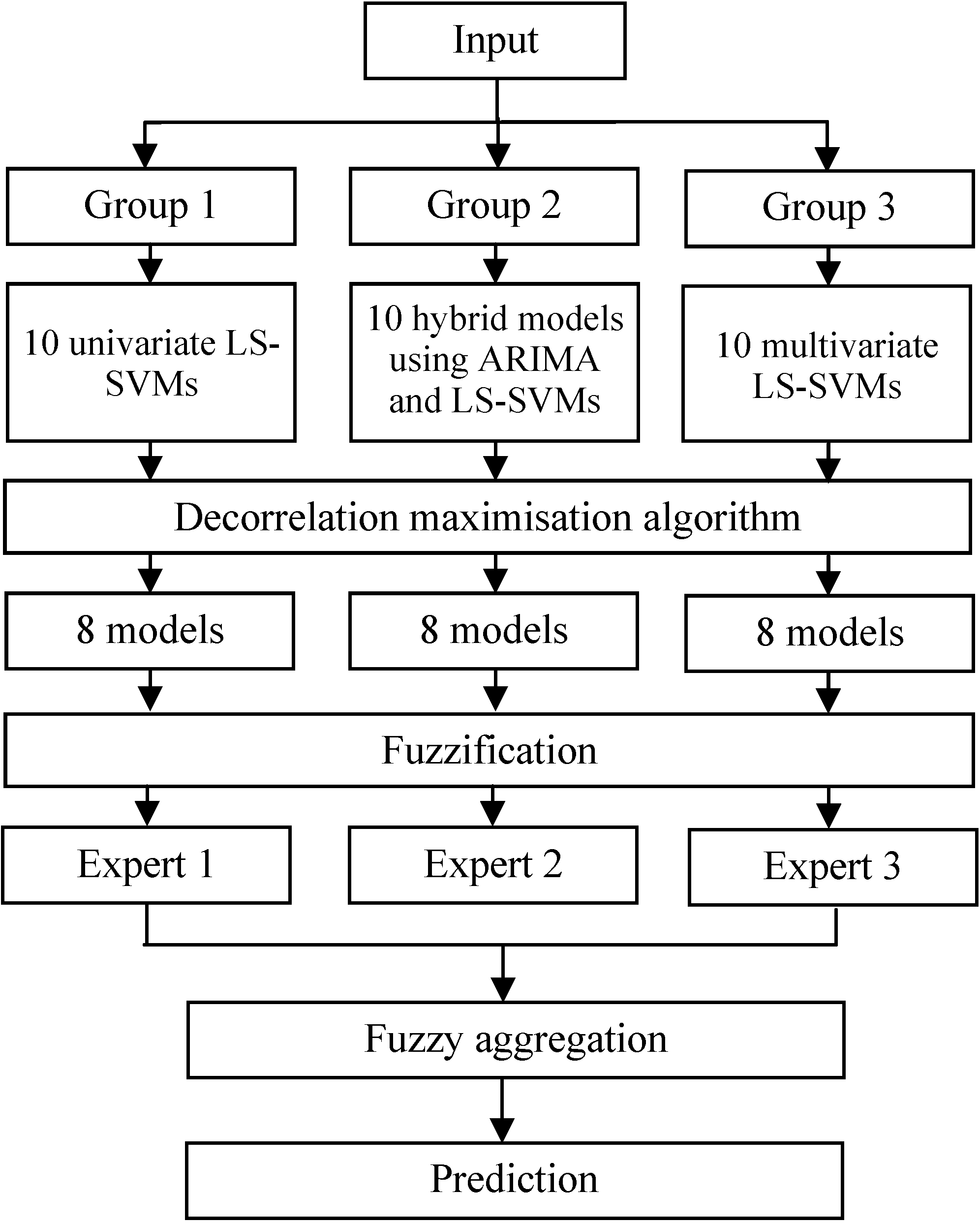
To illustrate and verify the proposed intelligent-agent-based fuzzy group forecasting model, the following section presents an illustrative numerical example of real-world data. The flow chart of the entire procedure is shown in Figure 1.

Figure 1. Procedure flow chart.

Figure 1. Procedure flow chart.

3. Empirical Analyses

3.1. Forecasting Results

In this study, we collected wind power output data from the Changshun wind park in Huade County, Inner Mongolia Autonomous Region, China. This wind park is located on the slopes of hills and mountains within an area of 260 km². Details of the park’s geographical information are provided in Table 4. This wind park was completed in May 2010 and has a capacity of 49.5 MW. Its wind power-out data from 1 January 2011, to 31 December 2011, were collected as shown in Figure 2. The short-term forecasting model for predicting hourly power output over a 24-hour horizon was tested. Other input data, such as the actual climate information, were collected from local environmental stations.

Table 4. Wind park geographical information.

Latitude (North)	Longitude (East)	Elevation (m)	Wind speed (m/s)		Temperature (°C)
			Mean	Max	Mean	Min	Max
41°10'–41°45'	113°49'–114°03'	1500	4.8	29	2.2	−35.9	35.5

Note: The very low minimum temperature is the extremely low temperature in this area, the lowest temperatures in this wind park is −27 °C in January. There is no stop in 2011 due to low temperature.

Table 4. Wind park geographical information.

Latitude (North)	Longitude (East)	Elevation (m)	Wind speed (m/s)		Temperature (°C)
			Mean	Max	Mean	Min	Max
41°10'–41°45'	113°49'–114°03'	1500	4.8	29	2.2	−35.9	35.5

Note: The very low minimum temperature is the extremely low temperature in this area, the lowest temperatures in this wind park is −27 °C in January. There is no stop in 2011 due to low temperature.

Figure 2. Time series plots of hourly wind power output.

Figure 2. Time series plots of hourly wind power output.

The data from 1 January 2011, to 31 October 2011, are used for constructing and training the models. The data from November 2011 are used to test the models and select the group modes according to Section 2.3. The results are presented in Table 5.

The data from December 2011 are used in the testing of the models and in the model analysis. There are 24 points for each day. To judge the accuracy of the model, individual models and the combined fuzzy forecasting model are compared using the following MAPE:

(28)

where ${\widehat{p}}_i$ is the forecast data, p_i is the real-time data, and N is the number of time points used in determining the forecast.

Also the relative error is adopted to evaluate the models performance. The error is calculated as the follows:

$$RE=\frac{p_i-{\widehat{p}}_i}{p_i}\times 100\%$$

(29)

The MAPEs of the individual models and the combined fuzzy forecasting model are calculated. The results are shown in Table 5.

Table 5. The MAPEs of individual models and the combined fuzzy forecasting model.

Group 1		Group 2		Group 3
model	MAPE	model	MAPE	model	MAPE
LS-SVM-1	19.71%	H-AR-LS-1	17.26%	DLS-SVM-1	18.06%
LS-SVM-2	24.03%	H-AR-LS-2	21.22%	DLS-SVM-2	21.91%
LS-SVM-3	24.75%	H-AR-LS-3	21.85%	DLS-SVM-3	20.65%
LS-SVM-4	19.52%	H-AR-LS-4	18.05%	DLS-SVM-4	17.62%
LS-SVM-6	18.94%	H-AR-LS-5	17.46%	DLS-SVM-5	20.85%
LS-SVM-7	25.36%	H-AR-LS-6	18.50%	DLS-SVM-6	16.71%
LS-SVM-9	22.45%	H-AR-LS-7	16.99%	DLS-SVM-9	18.31%
LS-SVM-10	18.08%	H-AR-LS-10	19.01%	DLS-SVM-10	22.35%
Average	21.61%	Average	18.79%	Average	19.56%
GFSVM	15.27%

Table 5. The MAPEs of individual models and the combined fuzzy forecasting model.

Group 1		Group 2		Group 3
model	MAPE	model	MAPE	model	MAPE
LS-SVM-1	19.71%	H-AR-LS-1	17.26%	DLS-SVM-1	18.06%
LS-SVM-2	24.03%	H-AR-LS-2	21.22%	DLS-SVM-2	21.91%
LS-SVM-3	24.75%	H-AR-LS-3	21.85%	DLS-SVM-3	20.65%
LS-SVM-4	19.52%	H-AR-LS-4	18.05%	DLS-SVM-4	17.62%
LS-SVM-6	18.94%	H-AR-LS-5	17.46%	DLS-SVM-5	20.85%
LS-SVM-7	25.36%	H-AR-LS-6	18.50%	DLS-SVM-6	16.71%
LS-SVM-9	22.45%	H-AR-LS-7	16.99%	DLS-SVM-9	18.31%
LS-SVM-10	18.08%	H-AR-LS-10	19.01%	DLS-SVM-10	22.35%
Average	21.61%	Average	18.79%	Average	19.56%
GFSVM	15.27%

3.2. Statistical Test

The best individual model is DLS-SVM-6, and the second best is H-AR-LS-7 in terms of MAPE, Statistical test is carried out among the GFSVM model and those two models. According to the methods mentioned in reference [27], comparison in made between the GFSVM model and the best individual model DLS-SVM-6.

${\left\{y_{it}\right\}}_{t=1}^T$ is the history data series, ${\left\{{\widehat{y}}_{it}\right\}}_{t=1}^T$ is the results from the GFSVM model, ${\left\{{\widehat{y}}_{jt}\right\}}_{t=1}^T$ is the result from the DLS-SVM-6 model. ${\left\{e_{it}\right\}}_{t=1}^T$ is the error of GFSVM model and ${\left\{e_{jt}\right\}}_{t=1}^T$ is the error of DLS-SVM-6 model. The loss function will be a direct function of the forecast error, that is $g(y_t,{\widehat{y}}_{it})=g(e_{it})$. The loss differential is $d_t=[g(e_{it})-g(e_{jt})]$. Empirically, the forecast error has many features: 1. zero mean 2, Gaussian 3. Serially correlated 4 contemporaneously correlated. The null hypothesis is a positive median loss differential: med(g(e_it) − g(e_jt)) < 0. So, we introduce two test statistics in reference [27], S₁ and S_2a as the follows:

(30)

(31)

(32)

(33)

(34)

where ${\widehat{f}}_d(0)$ is a consistent estimate of $f_d(0)$:

(35)

(36)

where I₊(d_t) = 1 if d_t > 0; I₊(d_t) = 0 otherwise:

$$S_{2a}=\frac{S_2-0.5T}{\sqrt{0.25T}}\stackrel{a}{\to }N\left(0,1\right)$$

(37)

The comparison result between the GFSVM model and DLS-SVM-6 the model is shown as Figure 3 and Table 6.

The same comparison is made between the GFSVM model and the H-AR-LS-7 model, and the result is shown as Figure 4 and Table 7.

In Table 6 and Table 7, T is sample size, ρ is the contemporaneous correlation, and θ is the serial correlation. All tests are at the 10% level. We perform 260 replications.

For comparison between the GFSVM model and the DLS-SVM-6 model, we obtain S₁ = 11.74, S_2a = 10.67 which implying a p-value= 0.089, 0.076. Thus, for sample at hand we do not reject at conventional level the hypothesis of the accuracy of the GFSVM model is better than the DLS-SVM-6 model. In the similar way, we can also statistically conclude that the GFSVM model is better than the H-AR-LS-7 model.

From above, we can draw a statistical conclusion that the GFSVM model is better than the DLS-SVM-6 model and the H-AR-LS-7 model.

Figure 3. Loss Differential (GFSVM - DLS-SVM-6).

Figure 3. Loss Differential (GFSVM - DLS-SVM-6).

Table 6. Empirical Size under Quadratic Loss, Test Statistic S₁, S_2a (GFSVM—DLS-SVM-6).

		S1			S2a
T	ρ	θ = 0	θ = 0.5	θ = 0.9	θ = 0	θ = 0.5	θ = 0.9
168	0	11.47	11.72	11.89	10.93	10.96	11.06
168	0.5	11.26	11.62	11.41	10.84	10.94	11.11
168	0.9	11.53	11.08	11.17	10.41	11.03	10.92

Table 6. Empirical Size under Quadratic Loss, Test Statistic S₁, S_2a (GFSVM—DLS-SVM-6).

		S1			S2a
T	ρ	θ = 0	θ = 0.5	θ = 0.9	θ = 0	θ = 0.5	θ = 0.9
168	0	11.47	11.72	11.89	10.93	10.96	11.06
168	0.5	11.26	11.62	11.41	10.84	10.94	11.11
168	0.9	11.53	11.08	11.17	10.41	11.03	10.92

Figure 4. Loss Differential (GFSVM - H-AR-LS-7).

Figure 4. Loss Differential (GFSVM - H-AR-LS-7).

Table 7. Empirical Size under Quadratic Loss, Test Statistic S₁, S_2a (GFSVM—H-AR-LS-7).

		S1			S2a
T	ρ	θ = 0	θ = 0.5	θ = 0.9	θ = 0	θ = 0.5	θ = 0.9
168	0	11.45	11.69	11.78	10.87	10.91	11.13
168	0.5	11.23	11.61	11.37	10.81	10.97	11.12
168	0.9	11.54	11.11	11.15	10.38	10.92.	10.97

Table 7. Empirical Size under Quadratic Loss, Test Statistic S₁, S_2a (GFSVM—H-AR-LS-7).

		S1			S2a
T	ρ	θ = 0	θ = 0.5	θ = 0.9	θ = 0	θ = 0.5	θ = 0.9
168	0	11.45	11.69	11.78	10.87	10.91	11.13
168	0.5	11.23	11.61	11.37	10.81	10.97	11.12
168	0.9	11.54	11.11	11.15	10.38	10.92.	10.97

3.3. Result Discussions

From Table 5, it can be observed that the fuzzy group forecasting model (GFSVM) performs best in terms of MAPE, with a MAPE of only 15.27%. The average MAPEs of these 8 models for groups 1, 2 and 3 are 21.61, 18.79 and 19.6%, respectively; all of these MAPEs are higher than those of the GFSVM. The best and second best individual models are DLS-SVM-6 and H-AR-LS-7, and their relative errors for total testing points are shown in Figure 5 and Figure 6 respectively. From these two figures, it can be observed that the range of the relative errors from the fuzzy group forecasting model GFSVM is smaller than that for DLS-SVM-6 and H-AR-LS-7. This means that the GFSVM is much more reliable than the other models. Table 8 represents the number of predictions between ±10%, ±20%, ±30% and ±40% for DLS-SVM-6, H-AR-LS-7 and GFSVM. For example, for the GFSVM model, 47.3% of the predictions have errors between ±10%, whereas for the DLS-SVM-6 model, 34.1% of the errors are in the same error margin, and for H-AR-LS-7 model, only 30.5% of the errors are in the same error margin. Obviously, the accuracy of GFSVM model is the best among these three models. From Figure 7, we know that the GFSVM can imitate the actual wind power output with high accuracy.

Figure 5. Wind power forecast relative errors of GFSVM model and DLS-SVM-6 model.

Figure 5. Wind power forecast relative errors of GFSVM model and DLS-SVM-6 model.

Figure 6. Wind power forecast relative errors of GFSVM model and H-AR-LS-7model.

Figure 6. Wind power forecast relative errors of GFSVM model and H-AR-LS-7model.

Table 8. Wind power forecast errors distribution for three models (% of errors in each margin).

	GFSVM	DLS-SVM-6	H-AR-LS-7
±10%	47.3%	34.1%	30.5%
±20%	81.4%	76.6%	74.3%
±30%	98.2%	92.2%	91.6%
±40%	100.0%	100.0%	100.0%

Table 8. Wind power forecast errors distribution for three models (% of errors in each margin).

	GFSVM	DLS-SVM-6	H-AR-LS-7
±10%	47.3%	34.1%	30.5%
±20%	81.4%	76.6%	74.3%
±30%	98.2%	92.2%	91.6%
±40%	100.0%	100.0%	100.0%

Figure 7. Forecasts derived from the fuzzy model (2011, 12, 01-2011, 12, 07).

Figure 7. Forecasts derived from the fuzzy model (2011, 12, 01-2011, 12, 07).

It is found that there is correlations among the current wind power output and those 1 h before and later. It is feasible to use them for predicting. From the Statistical test, it can be proved that the performance of the GFSVM model is better than that of DLS-SVM-6 model and H-AR-LS-7 model. It is the best in terms of accuracy and reliability among the models of these three groups. Also its Robustness is higher than those of the LS-SVM, ARIMA LS-SVM, DLS-SVM models. The overall prediction of the proposed method is better, but there is still individual prediction with large error, which needs further research.

4. Conclusions

In this study, we integrated groups of models into an aggregated model by using fuzzy theory to improve forecasting performance. The fuzzy group model overcame the intrinsic defects of single models, obtained information from various single models, and then created the optimum combination. Therefore, in most cases, we can achieve the purpose of improving forecasting results by combination forecasting, which obviously improves accuracy. Combination forecasting can be used to forecast wind power output over short time horizons. Through imitation computation and comparison, we proved that the forecasting accuracy is improved. Our approach thus offers a new and effective method for wind power forecasting.

References

1. Liu, Y.; Kokko, A. Wind power in China: Policy and development challenges. Energy Policy 2010, 38, 5520–5529. [Google Scholar] [CrossRef]
2. Ramirez-Rosado, I.J.; Fernandez-Jimenez, L.A.; Monteiro, C.; Sousa, J.; Bessa, R. Comparison of two new short-term wind-power forecasting systems. Renew. Energy 2009, 34, 1848–1854. [Google Scholar] [CrossRef]
3. Kavasseri, R.G.; Seetharaman, K. Day-ahead wind speed forecasting using f-ARIMA models. Renew. Energy 2009, 34, 1388–1393. [Google Scholar] [CrossRef]
4. Costa, A.; Crespo, A.; Navarro, J.; Lizcano, G.; Madsen, H.; Feitosa, E. A review on the young history of the wind power short-term prediction. Renew. Sustain. Energy Rev. 2008, 12, 1725–1744. [Google Scholar] [CrossRef] [Green Version]
5. De Giorgi, M.G.; Ficarella, A.; Tarantino, M. Assessment of the benefits of numerical weather predictions in wind power forecasting based on statistical methods. Energy 2011, 36, 3968–3978. [Google Scholar] [CrossRef]
6. Ernst, B. Wind Power Prediction. In Wind Power in Power Systems, 2nd ed.; John Wiley & Sons, Ltd.: Chichester, UK, 2012; pp. 753–766. [Google Scholar]
7. Tol, R. Autoregressive conditional heteroscedasticity in daily wind speed measurements. Theor. Appl. Climatol. 1997, 56, 113–122. [Google Scholar] [CrossRef]
8. Torres, J.; Garcia, A.; de Blas, M.; de Francisco, A. Forecast of hourly average wind speed with ARMA models in Navarre (Spain). Sol. Energy 2005, 79, 65–77. [Google Scholar] [CrossRef]
9. Riahy, G.H.; Abedi, M. Short term wind speed forecasting for wind turbine applications using linear prediction method. Renew. Energy 2008, 33, 35–41. [Google Scholar] [CrossRef]
10. Atwa, Y.M.; El-Saadany, E.F. Annual wind speed estimation utilizing constrained grey predictor. IEEE Trans. Energy Conver. 2009, 24, 548–550. [Google Scholar] [CrossRef]
11. El-Fouly, T.H.M.; El-Saadany, E.F.; Salama, M.M.A. Grey predictor for wind energy conversion systems output power prediction. IEEE Trans. Power Syst. 2006, 21, 1450–1452. [Google Scholar] [CrossRef]
12. Lei, M.; Shiyan, L.; Chuanwen, J.; Hongling, L.; Yan, Z. A review on the forecasting of wind speed and generated power. Renew. Sustain. Energy Rev. 2009, 13, 915–920. [Google Scholar] [CrossRef]
13. Mohandes, M.A.; Halawani, T.O.; Rehman, S.; Hussain, A.A. Support vector machines for wind speed prediction. Renew. Energy 2004, 29, 939–947. [Google Scholar] [CrossRef]
14. Ul Haque, A.; Meng, J.L. Short-term wind speed forecasting based on fuzzy artmap. Int. J. Green Energy 2011, 8, 65–80. [Google Scholar] [CrossRef]
15. Hong, Y.Y.; Chang, H.L.; Chiu, C.S. Hour-ahead wind power and speed forecasting using simultaneous perturbation stochastic approximation (SPSA) algorithm and neural network with fuzzy inputs. Energy 2010, 35, 3870–3876. [Google Scholar] [CrossRef]
16. Fan, G.F.; Wang, W.S.; Liu, C.; Dai, H.Z. Wind Power Prediction Based on Artificial Neural Network; Electric Power Research Institute: Beijing, China, 2008; pp. 118–123. [Google Scholar]
17. Öztopal, A. Artificial neural network approach to spatial estimation of wind velocity data. Energy Convers. Manag. 2006, 47, 395–406. [Google Scholar] [CrossRef]
18. Ackermann, T. Wind power in power systems. Wind Eng. 2006, 30, 447–449. [Google Scholar]
19. Sánchez, I. Adaptive combination of forecasts with application to wind energy. Int. J. Forecast. 2008, 24, 679–693. [Google Scholar]
20. Nielsen, H.A.; Nielsen, T.S.; Madsen, H.; Pindado, M.J.; Marti, I. Optimal combination of wind power forecasts. Wind Energy 2007, 10, 471–482. [Google Scholar] [CrossRef]
21. Saini, L.; Soni, M. Artificial Neural Network based Peak Load Forecasting Using Levenberg-Marquardt and Quasi-Newton Methods. IEE Proc. Gener. Transm. Distrib. 2002, 149, 578–584. [Google Scholar] [CrossRef]
22. Du, Y.; Lu, J.; Li, Q.; Deng, Y. Short-term wind speed forecasting of wind farm based on least square-support vector machine. Power Syst. Technol. 2008, 32, 62–66. [Google Scholar]
23. Zhao, D.; Pang, W.; Zhang, J.S.; Wang, X. Based on Bayesian theory and online learning SVM for short term load forecasting. Proc. Chin. Soc. Electr. Eng. 2005, 25, 8–13. [Google Scholar]
24. Chen, P.Y.; Pedersen, T.; Bak-Jensen, B.; Chen, Z. ARIMA-based time series model of stochastic wind power generation. IEEE Trans. Power Syst. 2010, 25, 667–676. [Google Scholar] [CrossRef]
25. Eristi, H.; Demir, Y. A new algorithm for automatic classification of power quality events based on wavelet transform and SVM. Expert Syst. Appl. 2010, 37, 4094–4102. [Google Scholar] [CrossRef]
26. Zhang, G.P. Time series forecasting using a hybrid ARIMA and neural network model. Neurocomputing 2003, 50, 159–175. [Google Scholar] [CrossRef]
27. Diebold, F.X.; Mariano, R.S. Comparing predictive accuracy. J. Bus. Econ. Stat. 2002, 20, 134–144. [Google Scholar] [CrossRef]