A Method for Identification of Driving Patterns in Hybrid Electric Vehicles Based on a LVQ Neural Network

Abstract
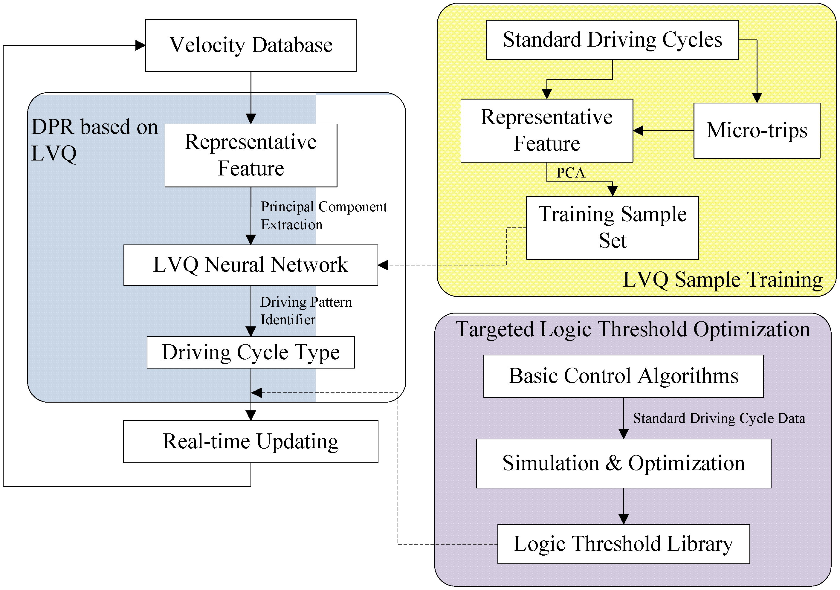
:1. Introduction

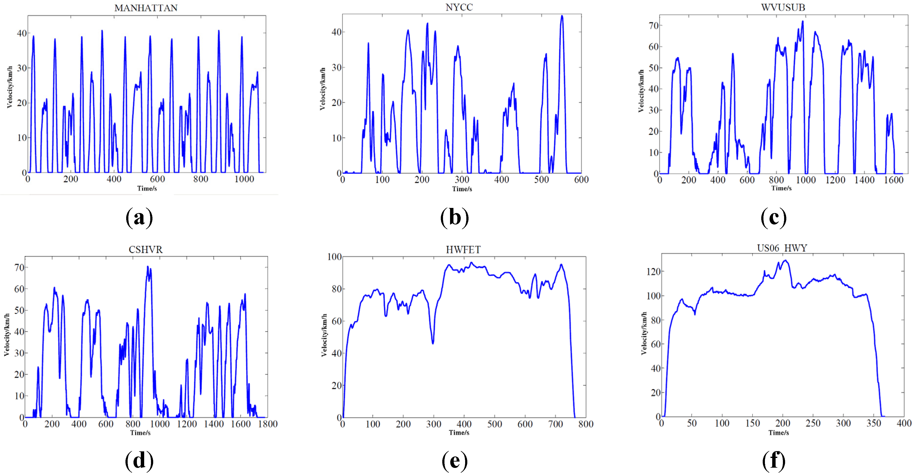
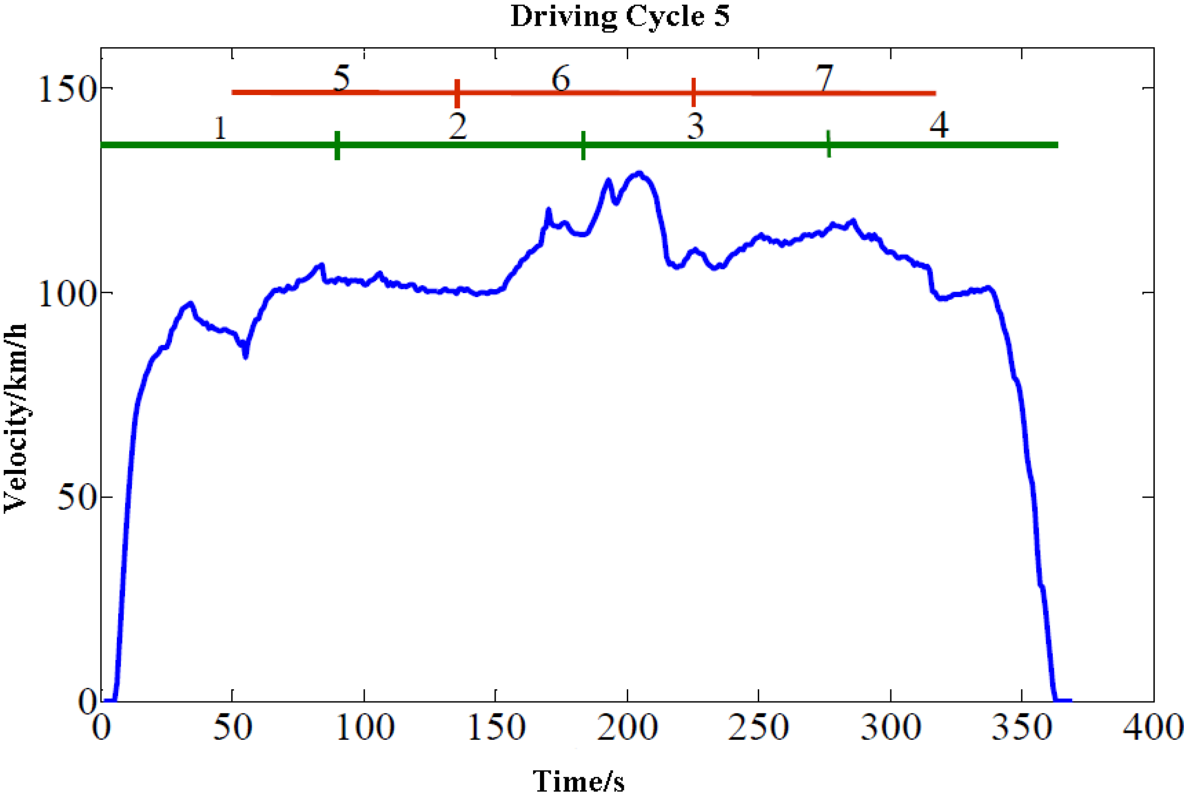
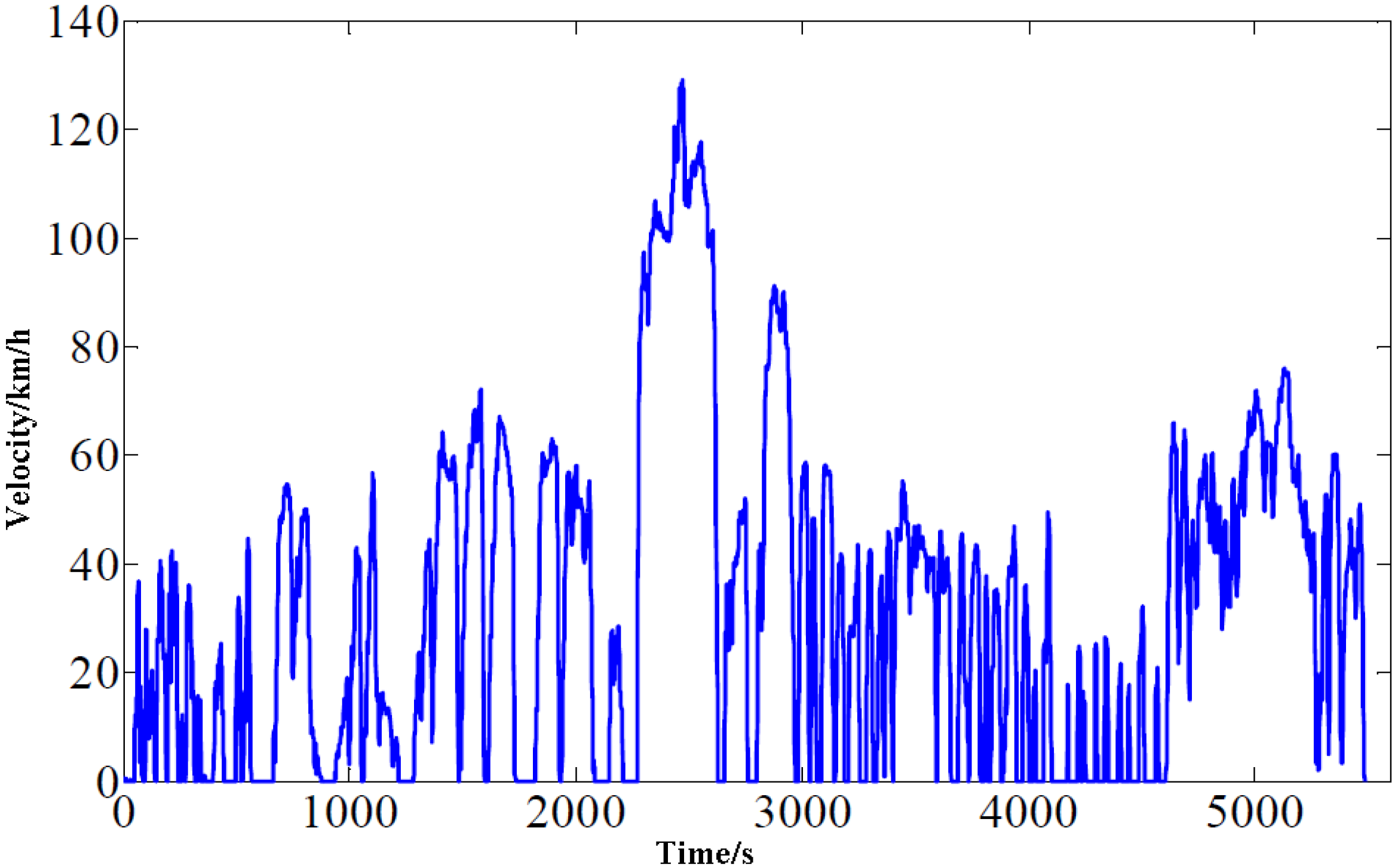
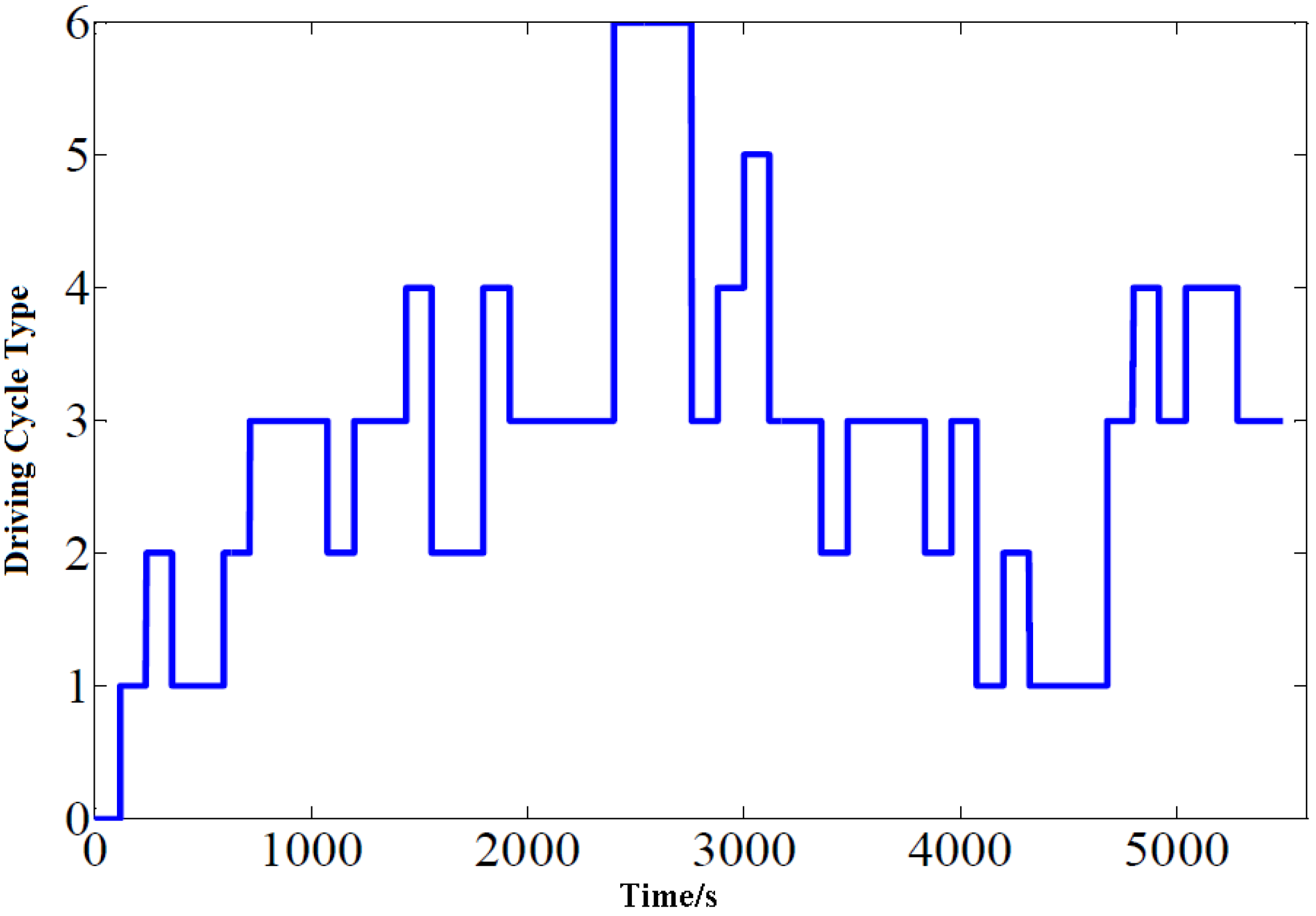
2. Driving Cycle Analysis and Training Sample Collection

| Driving Cycle Type | Name | Driving Cycle Number |
|---|---|---|
| Urban Road | MANHATTAN | Driving Cycle 1 |
| NYCC | Driving Cycle 2 | |
| Suburb Road | WVUSUB | Driving Cycle 3 |
| CSHVR | Driving Cycle 4 | |
| Highway Road | HWFET | Driving Cycle 5 |
| HS06_HWY | Driving Cycle 6 |

2.1. Representative Feature Analysis for DPR
2.1.1. Representative Features
| MANHATTAN | NYCC | WVUSUB | CSHVR | HWFET | US06_HWY | |
|---|---|---|---|---|---|---|
| 10.98 | 11.41 | 25.87 | 21.86 | 77.58 | 97.91 | |
| 40.72 | 44.58 | 72.10 | 70.49 | 96.40 | 129.23 | |
| 2.06 | 2.68 | 1.29 | 1.16 | 1.43 | 3.08 | |
| −2.5 | −2.64 | −2.16 | −1.79 | −1.48 | −3.08 | |
| 0.54 | 0.62 | 0.33 | 0.39 | 0.19 | 0.34 | |
| −0.67 | −0.61 | −0.42 | −0.46 | −0.22 | −0.41 | |
| 36.18% | 35.12% | 25.23% | 21.63% | 0.78% | 3.26% |
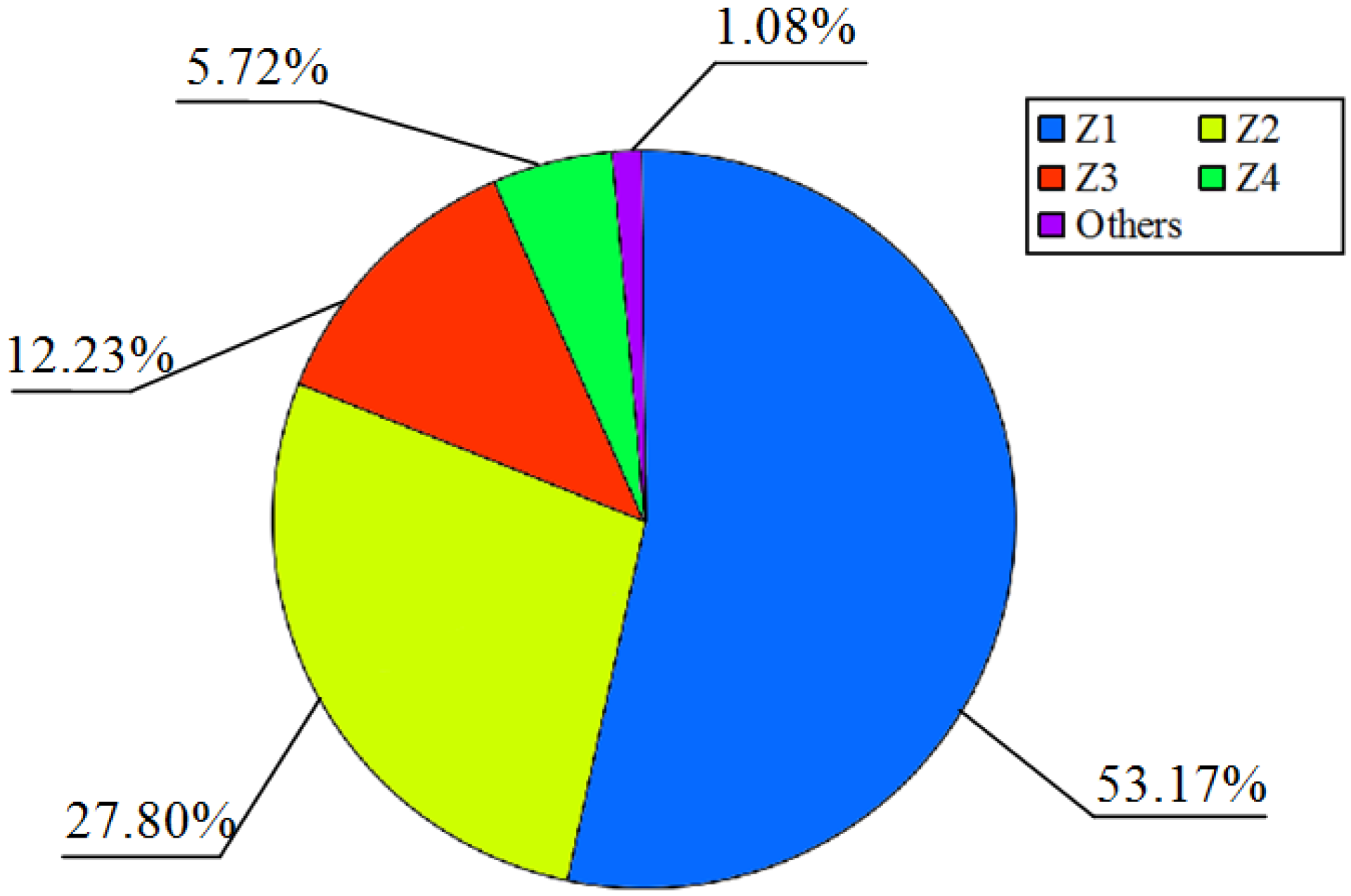
2.1.2. Principal Component Analysis

| aij | x1 | x2 | x3 | x4 | x5 | x6 |
|---|---|---|---|---|---|---|
| Z1 | −0.4161 | 0.3039 | 0.1756 | −0.2419 | −0.4373 | 0.6574 |
| Z2 | −0.4181 | 0.2808 | −0.3934 | −0.1847 | 0.6006 | 0.1368 |
| Z3 | 0.0801 | 0.6356 | 0.5199 | 0.2099 | −0.0885 | −0.2639 |
| Z4 | −0.1655 | −0.5997 | 0.5562 | −0.2915 | 0.1059 | 0.0873 |
| Z5 | 0.4481 | 0.1735 | 0.3656 | −0.1302 | 0.5942 | 0.3736 |
| Z6 | −0.4516 | −0.1502 | 0.2040 | 0.7894 | 0.2349 | 0.1333 |
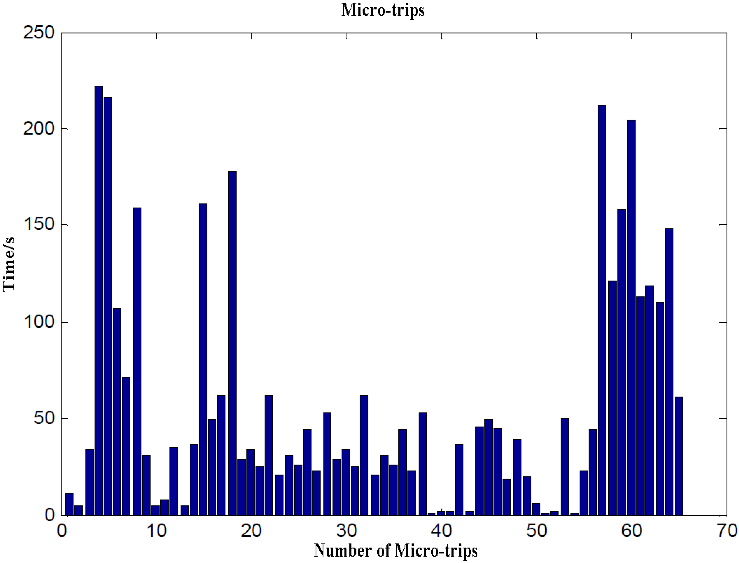
2.2. Micro-Trip Extraction and Sample Collection
3. Driving Pattern Recognition based on LVQ Neural Network
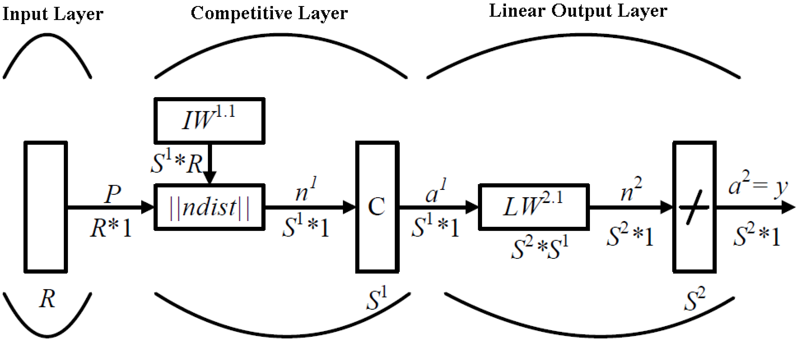
3.1. LVQ Neural Network

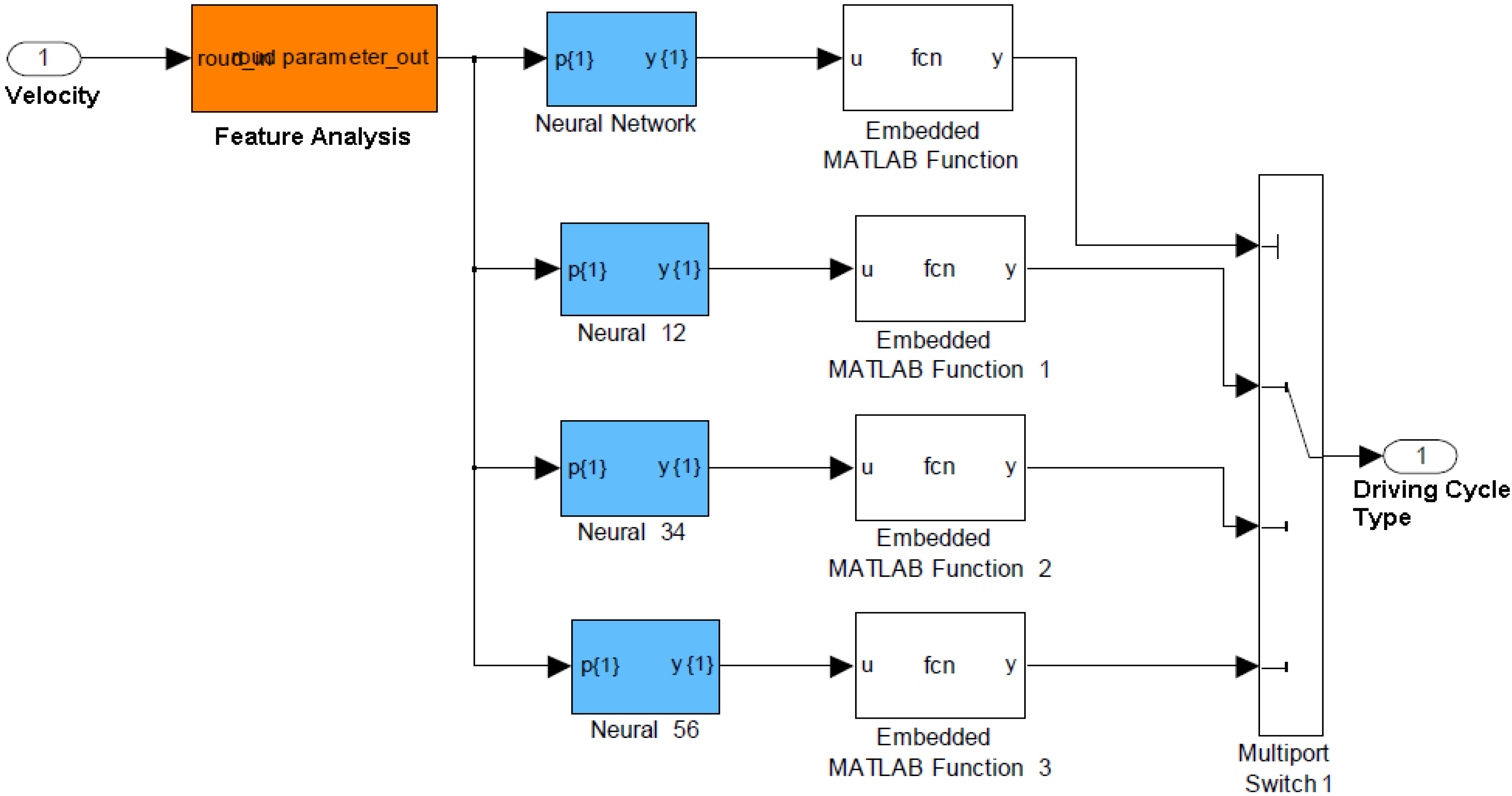
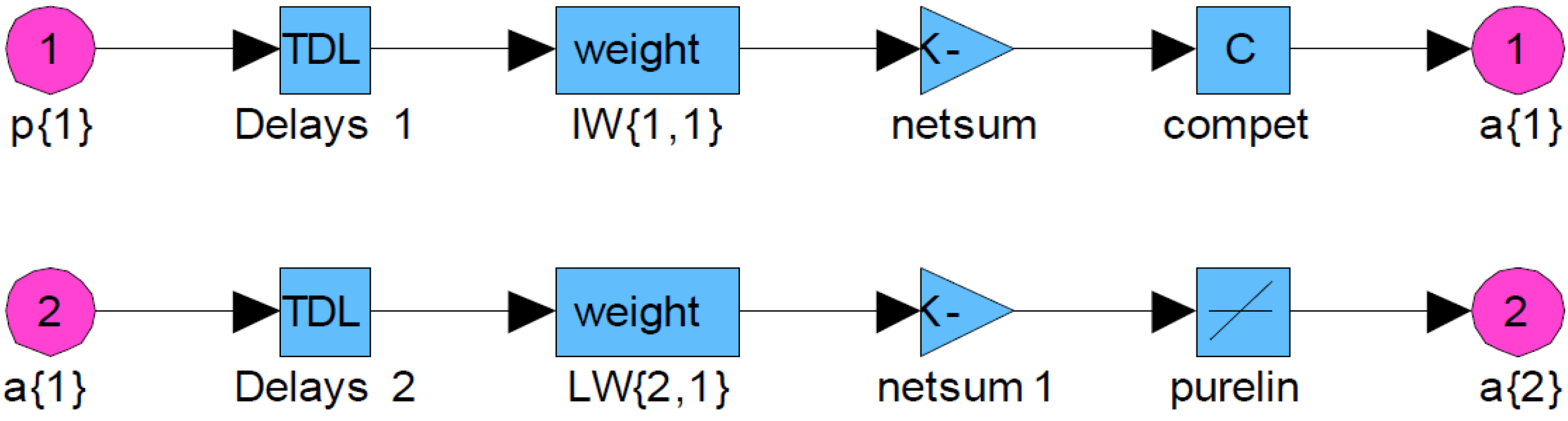
3.2. Driving Pattern Identifier Model
3.2.1. Model Structure

3.2.2. Sample Training

- (1)
- Neuron m and neuron n correspond with different patterns or categories;
- (2)
- The distances (to input vector) and meet Equation (15):where —the window width that the input vector may fall into , usually about 2/3.
3.3. Identifier Model Verification
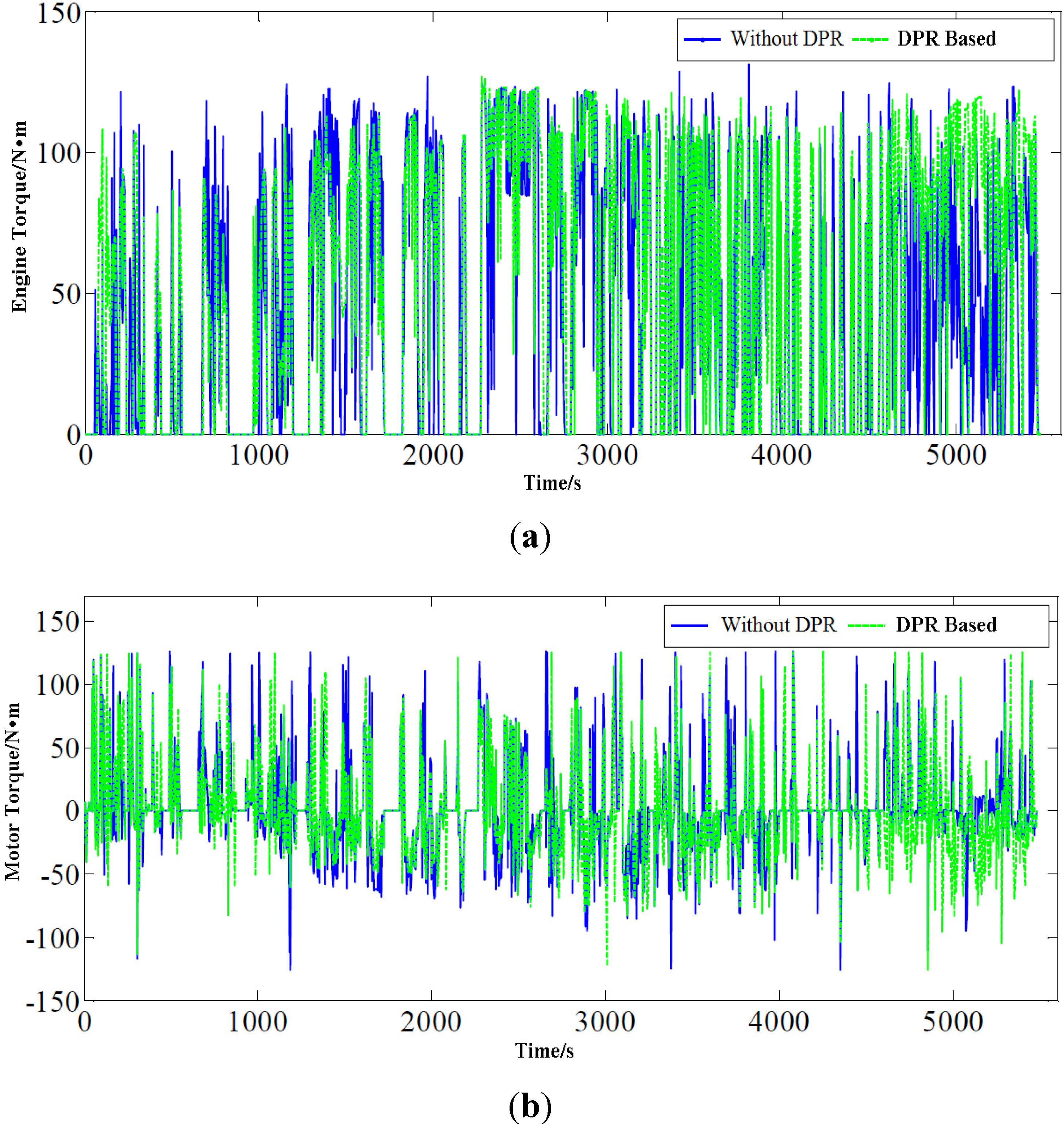
4. Simulation Experiment on the DPR Application
| System | Parameter | Value |
|---|---|---|
| Vehicle | Curb Weight | 3025 kg |
| Front Face Area | 3.042 m2 | |
| Rolling Resistance | 0.008 | |
| Air Resistance | 0.4 | |
| Transmission Efficiency | 0.90 | |
| Driving Wheel Rolling Radius | 0.325 m | |
| AMT | Gear Ratio | [4.452, 2.269, 1.517, 1, 0.854] |
| Engine | Maximum Power Rating | 76 kW/6000 |
| Torque Capacity | 131 N/5000 | |
| Motor | Motor Type | PMSM |
| Nominal Power Capacity | 10 kW | |
| Peak Power Capacity | 24 kW | |
| Battery | Battery Type | Lithium Iron Phosphate |
| Nominal Voltage | 336 V | |
| Nominal Capacity | 20 Ah |


| NYCC Optimized | DPR Optimized | |
|---|---|---|
| Fuel Consumption | 10.22 L/100km | 9.35 L/100km |
| Reduction Ratio | 0.0% | 8.51% |
5. Conclusions
- (1)
- A micro-trip extraction method is used to optimize the training of the LVQ identifier. The amount of training samples is substantially increased and the velocity sampling window length of DPR is reduced within 120 s. As a result, the sampling time is reduced during a recognition process;
- (2)
- Principal Component Analysis (PCA) method is used to optimize the calculation burden of the LVQ identifier. The four principal components extracted from the seven representative features act as the inputs of the LVQ neural network. As a result, the computing space and time of LVQ identifier is reduced and the identification accuracy can still be safeguarded;
- (3)
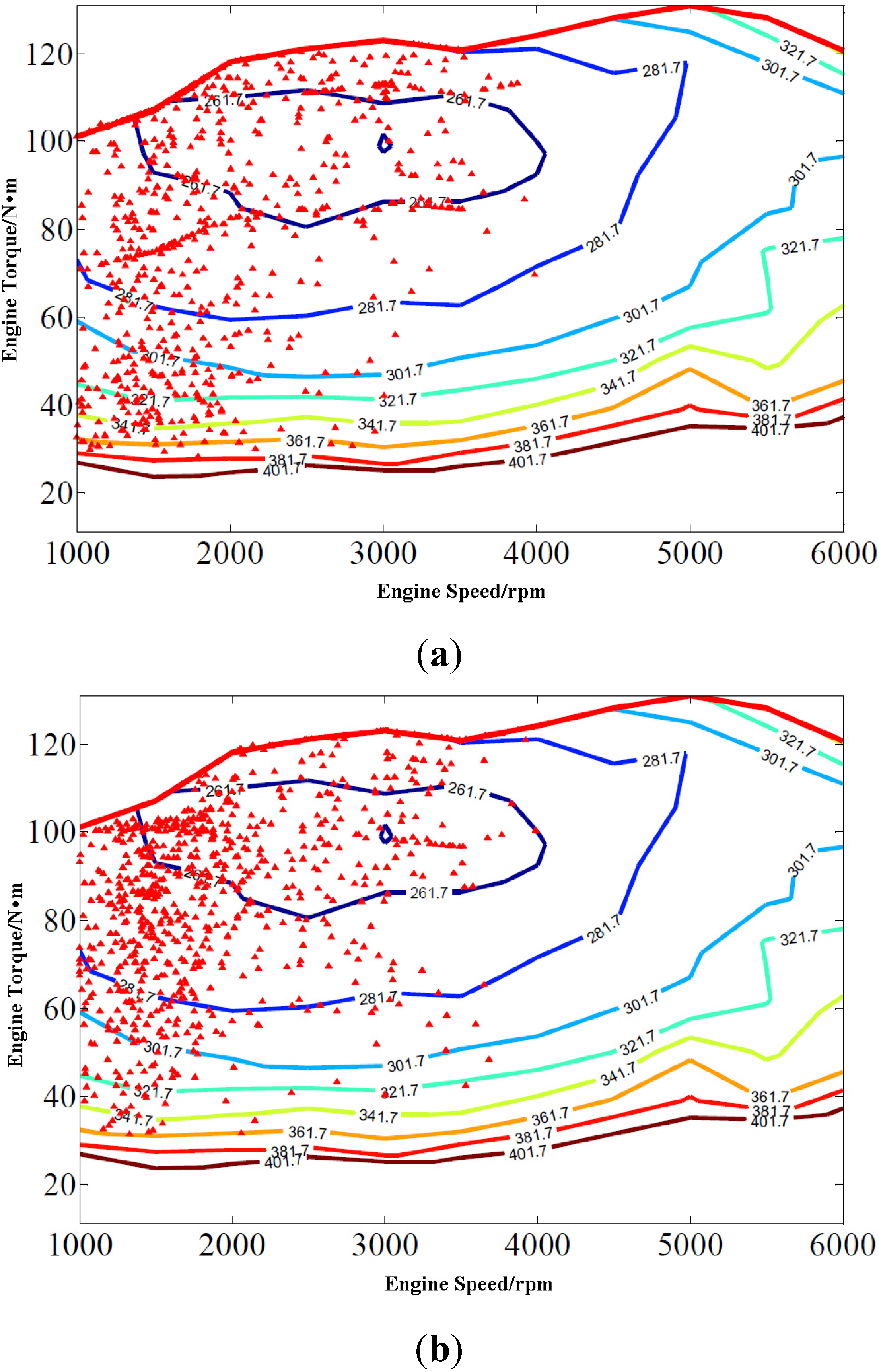
- Co-simulation of the LVQ driving pattern identifier together with a parallel HEV model is conducted. Simulation results show that the engine works in high-efficiency areas more frequently and the fuel economy can be improved by up to 8.51%.
Acknowledgements
References
- Chan, C.C. The state of the art of electric, hybrid, and fuel cell vehicles. Proc. IEEE 2007, 95, 704–718. [Google Scholar] [CrossRef]
- Abdelsalam, A.; Cui, S. A fuzzy logic global power management strategy for hybrid electric vehicles based on a permanent magnet electric variable transmission. Energies 2012, 5, 1175–1198. [Google Scholar] [CrossRef]
- Gurkaynak, Y.; Khaligh, A.; Emadi, A. State of the Art Power Management Algorithms for Hybrid Electric Vehicles. In Proceedings of the IEEE Vehicle Power and Propulsion Conference, Dearborn, MI, USA, 7–10 September 2009; pp. 388–394.
- Jeon, S.I.; Jo, S.T.; Park, Y.I.; Lee, J.M. Multimode driving control of a parallel hybrid electric vehicle using driving pattern recognition. J. Dyn. Syst. Meas. Control 2002, 124, 141–149. [Google Scholar] [CrossRef]
- Lin, C.C.; Jeon, S.; Peng, H.; Lee, J.M. Driving pattern recognition for control of hybrid electric trucks. Veh. Syst. Dyn.: Int. J. Veh. Mech. Mobil. 2004, 42, 41–58. [Google Scholar] [CrossRef]
- Musardo, C.; Rizzoni, G.; Staccia, B. A-ECMS: An Adaptive Algorithm for Hybrid Electric Vehicle Energy Management. In Proceedings of the 44th IEEE Conference on Decision and Control, Seville, Spain, 12–15 December 2005; pp. 1816–1823.
- Gong, Q.M.; Li, Y.Y.; Peng, Z.R. Power Management of Plug-in Hybrid Electric Vehicles Using Neural Network based Trip Modeling. In Proceedings of the American Control Conference, St. Louis, MI, USA, 10–12 June 2009; pp. 4601–4606.
- Zhang, C.; Vahidi, A. Role of terrain preview in energy management of hybrid electric vehicles. IEEE Trans. Veh. Technol. 2010, 59, 1139–1147. [Google Scholar] [CrossRef]
- Wang, R.; Lukic, S.M. Review of Driving Conditions Prediction and Driving Style Recognition Based Control Algorithms for Hybrid Electric Vehicles. In Proceedings of the 2011 IEEE Vehicle Power and Propulsion Conference (VPPC), Chicago, IL, USA, 6–9 September 2011; Volume 1, pp. 1–7.
- Won, J.S.; Langari, R. Intelligent energy management agent for a parallel hybrid vehicle—Part II: Torque distribution, charge sustenance strategies, and performance results. IEEE Trans. Veh. Technol. 2005, 54, 935–953. [Google Scholar] [CrossRef]
- Langari, R.; Won, J.S. Integrated Drive Cycle Analysis for Fuzzy Logic Based Energy Management in Hybrid Vehicles. In Proceedings of the 12th IEEE International Conference on Fuzzy Systems, St. Louis, MI, USA, 25–28 May 2003; pp. 290–295.
- Won, J.S.; Langari, R. Intelligent energy management agent for a parallel hybrid vehicle—Part I: System architecture and design of the driving situation identification process. IEEE Trans. Veh. Technol. 2005, 54, 925–934. [Google Scholar] [CrossRef]
- Lei, F.; Liu, W.; Chen, B. Driving pattern recognition for adaptive hybrid vehicle control. SAE Tech. Paper 2012. [Google Scholar] [CrossRef]
- Press, W.H.; Teukolsky, S.A. The Art of Scientific Computing, 3rd ed.; Cambridge University Press: New York, NY, USA, 2007; pp. 840–883. [Google Scholar]
- Ericsson, E. Independent driving pattern factors and their influence on fuel-use and exhaust emission factors. Transp. Res. Part D Transp. Environ. 2001, 6, 325–345. [Google Scholar] [CrossRef]
- Tian, Y.; Zhang, X.; Zhang, L. Intelligent Energy Management Based on Driving Cycle Identification Using Fuzzy Neural Network. In Proceedings of the 2nd International Symposium on Computational Intelligence and Design, Changsha, China, 12–14 December 2009; Volume 2, pp. 501–504.
- Montazeri-Gh, M.; Asadi, M. Intelligent approach for parallel HEV control strategy based on driving cycles. Int. J. Syst. Sci. 2011, 42, 287–302. [Google Scholar] [CrossRef]
- Montazeri, M.; Fotouhi, A.; Naderpour, A. Driving segment simulation for determination of the most effective driving features for HEV intelligent control. Veh. Syst. Dyn.: Int. J. Veh. Mech. Mobil. 2012, 50, 229–246. [Google Scholar] [CrossRef]
- Langari, R.; Won, J.S. A driving situation awareness-based energy management strategy for parallel hybrid vehicles. SAE Trans. 2003, 112, 1938–1947. [Google Scholar]
- Xing, J. Study on HEV Genetic-Fuzzy Control Strategy Based On Driving Cycle Recognition. Ph.D. Thesis, Beijing Institute of Technology, Beijing, China, 2010. [Google Scholar]
- Mehrotra, K.; Mohan, C.K.; Ranka, S. Elements of Artificial Neural Networks; MIT Press: Cambridge, MA, USA, 1997; pp. 173–180. [Google Scholar]
- Chen, H.Y.; Wu, G.Q. Compensation fuzzy neural network power management strategy for hybrid electric vehicle. J. Tongji Univ. (Nat. Sci.) 2009, 37, 525–530. [Google Scholar]
- Shi, Z.Z. Neural Networks, 1st ed.; Higher Education Press: Beijing, China, 2009; pp. 152–169. [Google Scholar]
- He, H.; Liu, Z.; Zhu, L.; Liu, X. Dynamic coordinated shifting control of automated mechanical transmissions without a clutch in a plug-in hybrid electric vehicle. Energies 2012, 5, 3094–3109. [Google Scholar] [CrossRef]
© 2012 by the authors; licensee MDPI, Basel, Switzerland. This article is an open access article distributed under the terms and conditions of the Creative Commons Attribution license (http://creativecommons.org/licenses/by/3.0/).
Share and Cite
He, H.; Sun, C.; Zhang, X. A Method for Identification of Driving Patterns in Hybrid Electric Vehicles Based on a LVQ Neural Network. Energies 2012, 5, 3363-3380. https://doi.org/10.3390/en5093363
He H, Sun C, Zhang X. A Method for Identification of Driving Patterns in Hybrid Electric Vehicles Based on a LVQ Neural Network. Energies. 2012; 5(9):3363-3380. https://doi.org/10.3390/en5093363
Chicago/Turabian StyleHe, Hongwen, Chao Sun, and Xiaowei Zhang. 2012. "A Method for Identification of Driving Patterns in Hybrid Electric Vehicles Based on a LVQ Neural Network" Energies 5, no. 9: 3363-3380. https://doi.org/10.3390/en5093363