Evaluation of a Model for Predicting the Tidal Velocity in Fjord Entrances

Abstract

Sufficiently accurate and low-cost estimation of tidal velocities is of importance when evaluating a potential site for a tidal energy farm. Here we suggest and evaluate a model to calculate the tidal velocity in fjord entrances. The model is compared with tidal velocities from Acoustic Doppler Current Profiler (ADCP) measurements in the tidal channel Skarpsundet in Norway. The calculated velocity value from the model corresponded well with the measured cross-sectional average velocity, but was shown to underestimate the velocity in the centre of the channel. The effect of this was quantified by calculating the kinetic energy of the flow for a 14-day period. A numerical simulation using TELEMAC-2D was performed and validated with ADCP measurements. Velocity data from the simulation was used as input for calculating the kinetic energy at various locations in the channel. It was concluded that the model presented here is not accurate enough for assessing the tidal energy resource. However, the simplicity of the model was considered promising in the use of finding sites where further analyses can be made.

1. Introduction

Tidal current energy conversion is an emerging field of renewable energy. In Norway, with a coastline 83,000 km long, a tidal amplitude of ±1–2 m and numerous fjords along the coastline, there are many interesting sites for tidal energy development. Yet, little research has been made that evaluates the tidal stream energy resource in Norway. Grabbe et al. [1] reviewed the available reports on the tidal stream resource in Norway. The research documents an interesting potential for tidal energy. However, the estimates are highly insecure due to the questionable method used for the calculations and the lack of velocity data. For other resource assessments throughout the world, numerical models have been applied to estimate the velocity and sometimes the resource [2,3,4,5]. These models have increased the knowledge of the complex tidal regime in narrow channels where the hydrokinetic power is strong. As was pointed out by Grabbe et al. [1], various numerical models, calibrated with tidal level data, have been conducted in Norway before [6,7,8,9], however not for the use of estimating the tidal current resource.

To estimate the suitability of a site for tidal energy conversion, current measurement surveys are essential. Current measurement instruments, such as an Acoustic Doppler Current Profiler (ADCP), have been used for validating numerical models. This has been done for a river section [10], a fjord entrance [11] and other coastal areas [3,4,5,11]. The use of ADCP-measurements in the field of tidal energy resource estimation was discussed by Gooch, Thomson et al. [12] and Stiven et al. [13], where recommendations were given on how measurements should be conducted for a correct analysis.

Studies show that state-of-the-art for assessment of a tidal energy resource lies in advanced numerical models validated with velocity measurements. However, because these surveys are both costly and time-consuming, and due to the numerous areas with potential suitability for tidal energy extraction, a simpler, more generalised method is required for preliminary estimations. In this study a model for estimating the velocity in the entrance of a tidal fjord has been developed. The model requires only publicly available data. For the evaluation of the quality of the model, a site in a fjord entrance in Norway was studied. ADCP measurements were conducted and a numerical simulation using TELEMAC-2D was performed for the selected area. The main purpose is to evaluate the accuracy of predicting the tidal velocity in a fjord entrance using the presented model.

2. Site Description

The studied site, Skarpsundet, is situated in Norway and it connects the fjords Elsfjorden and Sørfjorden with Ranfjorden, at the approximate coordinates ${66}^{\circ }$${11}^{\prime }$ N ${13}^{\circ }$${36}^{\prime }$ E (Figure 1). The combined area of Elsfjorden and Sørfjorden is $38{\mathrm{km}}^2$.

Three rivers discharge into the fjord: Røssåga, Bjerka and Sannaelva. In the southwestern end of Sørfjorden the largest of the three rivers, Røssåga, is situated. It has a yearly average discharge of $115{\mathrm{m}}^3/\mathrm{s}$ [14]. However, the discharge of the rivers into the fjord system is small in comparison with the tidal flow, and has been neglected.

Figure 1. Overview map over Skarpsundet and surrounding fjords (map over Norway encapsulated).

Figure 1. Overview map over Skarpsundet and surrounding fjords (map over Norway encapsulated).

3. Methods

3.1. Estimation of $\widehat{u}$

When considering an enclosed area, such as a fjord, continuity implies that the volume change inside the bay must be equal to the flow into the bay. The flow into the bay consists of the flow through the channel that links the bay to the open ocean and other inputs such as river discharge. If the freshwater input is ignored, the continuity equation can be written as:

$$A_f\frac{d{h}_i}{dt}=Q$$

(1)

where $A_f$ is the area of the enclosed bay; $h_i$ is the water level inside the bay; and Q is the flow through the channel.

The total drop in water level over the channel is equal to $h_0-h_i$, where $h_0$ is the water level in the ocean on the outer side of the bay. This total drop in water level can be divided into two parts: one related to the friction in the channel ($\Delta h_f$) and one related to the acceleration of the flow toward the constriction ($\Delta h_b$) [15]. The frictional resistance can be modelled as a constant term multiplied with the square of the velocity. Several recent publications have modelled the constant term with different notations: Garrett and Cummins [16] used non-dimensionalised ${\lambda }_0$, Blanchfield et al. [17] used ${\lambda }_2$ and Atwater et al. [18] used the term k. It should be noted that in these publications an additional term was used, namely the friction induced by energy extraction from Tidal Energy Converters. In this study we only analysed the velocity in a tidal channel in the undisturbed state and thus the turbine extraction term was not included.

The frictional resistance can be calculated using the Manning number, n, according to

$$\Delta h_f=\frac{n^{2}L}{R^{4/3}}{\left(\frac{Q}{A_c}\right)}^2$$

(2)

where L is the length of the channel; R is the hydraulic radius; and $A_c$ is the cross-sectional area of the channel [19]. The variable $\Delta h_b$ can be written as:

$$\Delta h_b=\frac{Q^2}{2g{A}_c^2}$$

(3)

in which case the velocities outside the main channel are assumed to be negligible.

In the simplest case, the friction and acceleration term is considered negligible and only Equation (1) is applied to model the velocity in the sound. The water level inside the bay is then equal in amplitude to the water level outside. For large bays with relatively low velocity this is a valid assumption. The choking factor, here defined as:

$$C=100-\frac{h_{i,max}-h_{i,min}}{h_{0,max}-h_{0,min}}·100$$

(4)

can be used to analyse whether the friction in the channel can be ignored or not. This requires a numerical solution of Equations (1–3). For a choking factor close to zero, the assumption of a negligible friction is valid. In Figure 2a,b, the choking factor has been plotted against length and width of the channel, using a fjord area of $38{\mathrm{km}}^2$ (corresponding the Skarpsundet site), an ocean tidal amplitude of 2 m and a Manning number of 0.050. The choking factor increases with increased length of the channel and with decreased width (Figure 2). For a width of 300 m, the effect of choking will only affect the inner tidal water level by a few percent, whereas it will be strongly affected in channels that are less than 100 m wide, regardless of the length of the channel.

Figure 2. Choking factor (C) as a function of (a) width of the channel (W); and (b) length of the channel (L). The choking factor is defined as the range of the water level in the basin divided by the range of the water level in the open ocean.

Figure 2. Choking factor (C) as a function of (a) width of the channel (W); and (b) length of the channel (L). The choking factor is defined as the range of the water level in the basin divided by the range of the water level in the open ocean.

For the Skarpsundet site, the fjord area is $38{\mathrm{km}}^2$, the width of the channel is 700 m, and the length approximately 1000 m. The choking factor for this channel is zero and the drop in water level across the channel can be ignored. To estimate the velocity in the channel, only continuity is applied. Furthermore, assuming that the cross-sectional area will not change significantly during the tidal cycle, the flow will be dependent on the velocity in the channel such that $Q=A_c·u$. By this it is possible to get a relation between the velocity and the tidal level. Denoting the estimated velocity with $\widehat{u}$ the equation becomes:

$$\widehat{u}=\frac{A_f}{A_c}\frac{d{h}_i}{dt}$$

(5)

If the tidal water level has a sinusoidal variation with an angular frequency of ω, $h\left(t\right)=H_{max}sin\left(\omega t\right)$, the velocity will vary equally but with a phase shift, ϕ, of T/4, where T is the period of the tide, and a multiplier defined by $A_f/A_c·\omega$. In Norway the M2 tidal component is dominant and the period of the M2 tide is 12.42 h. A phase shift of T/4 thus corresponds to 3.1 h. This can be written as:

$$\widehat{u}\left(t\right)=\frac{A_f}{A_c}\omega h(t-\varphi )$$

(6)

$\omega =2\pi /T$=$1.4\times {10}^{-4}{\mathrm{s}}^{-1}$. The mean value is subtracted from the tidal level so that $h\left(t\right)$ varies around 0.

Björk et al. [20] estimated the velocity in the sound Malö Strömmar by using the water level difference on either side of the sound multiplied with a constant term. However, the constant term needed to be empirically measured. The purpose of this study is to evaluate how accurate a model is in sites where current measurements are absent.

Estimation of the Maximum Velocity

Equation (5) can be further extended to estimate the maximum velocity in the channel. Writing the sinusoidal variation of the velocity with $\widehat{u}\left(t\right)={\widehat{u}}_{max}sin\left(\omega t\right)$ the integration of Equation (5) over half a tidal period gives the maximum velocity:

$${\widehat{u}}_{max}=1.4·{10}^{-4}\left(s^{-1}\right)\frac{A_f}{A_c}\frac{H}{2}$$

(7)

where $H=h(T/2)-h\left(0\right)$, i.e., the change in water level from low to high tide or the tidal range.

The velocity and the maximum velocity can be estimated only knowing three parameters: the fjord area, the cross-sectional area of the fjord entrance and the tidal range. The calculation of the velocity is based on several assumptions, including the assumption that the friction and acceleration term is negligible. One assumption is that the freshwater input is ignored. This is valid in fjords or bays where the exchange caused by the tide is much larger than the freshwater input. Another assumption is that the water level inside the bay is equal everywhere. This assumption can be met in fjords that are much shorter than the length of the tidal wave. The length scale of long waves can be estimated with $l=T\sqrt{gH}$ [15]. For Norwegian fjords that are deep (often >100 m), the length of the tidal wave will be several hundred kilometres, which validates the assumption. Henceforth, only one velocity value will be given for each cross-section. The most questionable assumption is, however, that the cross-sectional area will not change with time. To come around this problem, the value of the cross-sectional area in Equations (6,7) is the value at maximum velocity.

Note that the model is a 1D-approach and following this, Equation (7) gives the cross-sectional average velocity.

3.2. Assessment of the Hydrokinetic Energy

The energy per unit area, E, during a time interval, t, have been calculated using the following equation:

$$E={\int }_0^t\frac{1}{2}\rho u^{3}dt$$

(8)

where $dt$ is a time step of 10 min; u is the velocity; and ρ is the density of the water.

3.3. Numerical Simulation

In order to analyse the velocity variations across the entire sound, the velocity was simulated using TELEMAC-2D [21]. The model was run with one open boundary where a tidal level series was applied for the free surface and a Thompson boundary condition for the velocity [21,22]. The tidal level was received from the Norwegian Hydrographic Service. A constant Strickler bottom friction value of 30 was used [21]. The model was then compared with measured ADCP-data. The mesh was created in Blue Kenue with 200 m size element in the larger area and 30 m in the sound (Figure 3). In other numerical models the grid size for slightly larger geometries varied in between 50 [22,23] and 150 m [3].

Table 1. Values for the Skarpsundet site.

Variable	Description	Value
ρ	Density	$1,025\mathrm{kg}/{\mathrm{m}}^3$
L	Length of Skarpsundet	$1,500\mathrm{m}$
$A_c$	Cross-sectional area	$13,500{\mathrm{m}}^2$
W	Average width of channel	$700\mathrm{m}$
H	Average depth of Skarpsundet	$15\mathrm{m}$
$A_f$	Fjord area	$3.8\times {10}^7{\mathrm{m}}^2$

Table 1. Values for the Skarpsundet site.

Variable	Description	Value
ρ	Density	$1,025\mathrm{kg}/{\mathrm{m}}^3$
L	Length of Skarpsundet	$1,500\mathrm{m}$
$A_c$	Cross-sectional area	$13,500{\mathrm{m}}^2$
W	Average width of channel	$700\mathrm{m}$
H	Average depth of Skarpsundet	$15\mathrm{m}$
$A_f$	Fjord area	$3.8\times {10}^7{\mathrm{m}}^2$

3.4. Bathymetry Measurement and Collection

The bathymetry of the site was investigated with a GPS and an echo-sounder (Eagle Cuda 168) in compliment to using available data from the Norwegian Mapping Authority [24]. Several transects were measured both across the channel and along the channel. Depth measurements were performed both on 23 May 2011 and 7 July 2011. The depth data were corrected to the sea-chart zero and compared with the available sea-chart data. It was later inserted in ArcMap to create a geometry for the numerical model and used to calculate the cross-sectional area of the channel.

Figure 3. Modelled area and mesh for the TELEMAC simulation. The Skarpsundet sound is shown within the square.

Figure 3. Modelled area and mesh for the TELEMAC simulation. The Skarpsundet sound is shown within the square.

3.5. Tidal Data Collection

Tidal data was received from the Norwegian Hydrographic Service (NHS) [25]. The tidal level from the NHS can be collected as predicted values, in which the tidal level is deduced from the harmonic constants, or observational values. The predicted values can be received from any location along the Norwegian coast, but the observational values are only present at any of the 23 available stations in Norway. The two water level measuring stations closest to Skarpsundet is in Rørvik located at ${64}^{\circ }{52}^{\prime }$ N, ${11}^{\circ }{15}^{\prime }$ E, approximately $180\mathrm{km}$ from Skarpsundet, and in Bodø located at ${67}^{\circ }{16}^{\prime }$ N, ${14}^{\circ }{22}^{\prime }$ E, $126\mathrm{km}$ from Skarpsundet. Tidal level characteristics deduced from the Rørvik and Bodø water level measuring stations is shown in Table 2 where the tidal levels are the mean spring tidal range, the mean high water range and the mean neap tidal range, defined as:

$$\begin{array}{cc}& H_{spring}=MHWS-MLWS\hfill \end{array}$$

(9)

$$\begin{array}{cc}& H_{mean}=MHW-MLW\hfill \end{array}$$

(10)

$$\begin{array}{cc}& H_{neap}=MHWN-MLWN\hfill \end{array}$$

(11)

Predicted tidal level with a time-interval of 10 min was received from the NHS for the site Skarpsundet.

Table 2. Tidal level characteristics from the Rørvik and Bodø water level measuring station.

Tidal range	Rørvik	Bodø
$H_{spring}$	212 cm	236 cm
$H_{mean}$	158 cm	174 cm
$H_{neap}$	103 cm	114 cm

Table 2. Tidal level characteristics from the Rørvik and Bodø water level measuring station.

Tidal range	Rørvik	Bodø
$H_{spring}$	212 cm	236 cm
$H_{mean}$	158 cm	174 cm
$H_{neap}$	103 cm	114 cm

3.6. ADCP Measurements

Velocity and tidal level data were measured using a 600 kHz ADCP Workhorse Sentinel from RD Instruments. The water level was measured with the built-in pressure sensor of the ADCP. One bottom mounted surveys and one transect measurement with a down-looking ADCP were performed. In Figure 4 the locations of the measurements are shown. Transect measurements are shown as black lines. The long-time measurement was performed during 43 days with a low-frequency sampling rate. Both are summarised in Table 3.

Figure 4. Bathymetry over Skarpsundet with the position of the bottom-mount measurement with the ADCP (# 1) and transect measurement (black lines) marked out.

Figure 4. Bathymetry over Skarpsundet with the position of the bottom-mount measurement with the ADCP (# 1) and transect measurement (black lines) marked out.

Table 3. Summary of the measurement survey in the strait of Skarpsundet, 2011. The geographical position of measurement #1 was ${66}^{\circ }{11}^{\prime }{53}^{″}\mathrm{N}$, ${13}^{\circ }{36}^{\prime }{43}^{″}\mathrm{E}$.

No.	Start		End		Frequency	Duration	Depth	Bin sz.
	Date	Time	Date	Time			(m)	(m)
# 1	24 May	15:10	7 July	09:10	$10\min$	$43\mathrm{day}$$18\mathrm{h}$	14.1–16.7	1
# 2	7 July	15:25	7 July	16:30	$15\mathrm{s}$	$1\mathrm{h}$$5\min$	5.5–22.4	1

Table 3. Summary of the measurement survey in the strait of Skarpsundet, 2011. The geographical position of measurement #1 was ${66}^{\circ }{11}^{\prime }{53}^{″}\mathrm{N}$, ${13}^{\circ }{36}^{\prime }{43}^{″}\mathrm{E}$.

No.	Start		End		Frequency	Duration	Depth	Bin sz.
	Date	Time	Date	Time			(m)	(m)
# 1	24 May	15:10	7 July	09:10	$10\min$	$43\mathrm{day}$$18\mathrm{h}$	14.1–16.7	1
# 2	7 July	15:25	7 July	16:30	$15\mathrm{s}$	$1\mathrm{h}$$5\min$	5.5–22.4	1

During the long-time measurement survey, there were a total of 84 tidal cycles being sampled.

During the transect measurement, the measurements occurred 4–5 h following low tide. A total of two transects were sampled. The speed of the boat was approximately 0.8 m/s. The cross-sound ADCP measurement occurred together with depth measurements with the echo-sounder and GPS. The combination of these measurements allowed for the creation of a horizontal velocity profile.

4. Results

4.1. Velocity and Tidal Level Data Results

The description of the data at different depth is presented in Table 4. The sustained maximum velocity [12] is here defined as the maximum velocity sustained for 20 min during the whole time series. Since measurements were collected every 10 min, this means a maximum of the average of two data points. Due to disturbances close to the surface, the top bins were removed, keeping only the bins measuring from 3 up to 11 m above the bottom.

Table 4. Statistics of the total, the flood and the ebb velocity for a few of the depths bins. z = height above bottom, $\overline{u}$ = mean velocity, $u_{max,sus}$ is the sustained maximum velocity [12] and θ is the average direction.

Flow	z	$\overline{\text{u}}$	${\text{u}}_{\max ,\mathrm{sus}}$	θ
	(m)	(m/s)	(m/s)	(degree)
	3	0.25	1.24	191
Total	6	0.32	1.13	199
	9	0.33	1.00	192
	all	0.31	1.10	194
	3	0.22	0.48	176
Flood	6	0.27	0.59	188
(incoming tide)	9	0.29	0.58	183
	all	0.27	0.60	184
	3	0.28	1.24	25
Ebb	6	0.37	1.13	31
(outgoing tide)	9	0.35	1.00	20
	all	0.34	1.09	23

Table 4. Statistics of the total, the flood and the ebb velocity for a few of the depths bins. z = height above bottom, $\overline{u}$ = mean velocity, $u_{max,sus}$ is the sustained maximum velocity [12] and θ is the average direction.

Flow	z	$\overline{\text{u}}$	${\text{u}}_{\max ,\mathrm{sus}}$	θ
	(m)	(m/s)	(m/s)	(degree)
	3	0.25	1.24	191
Total	6	0.32	1.13	199
	9	0.33	1.00	192
	all	0.31	1.10	194
	3	0.22	0.48	176
Flood	6	0.27	0.59	188
(incoming tide)	9	0.29	0.58	183
	all	0.27	0.60	184
	3	0.28	1.24	25
Ebb	6	0.37	1.13	31
(outgoing tide)	9	0.35	1.00	20
	all	0.34	1.09	23

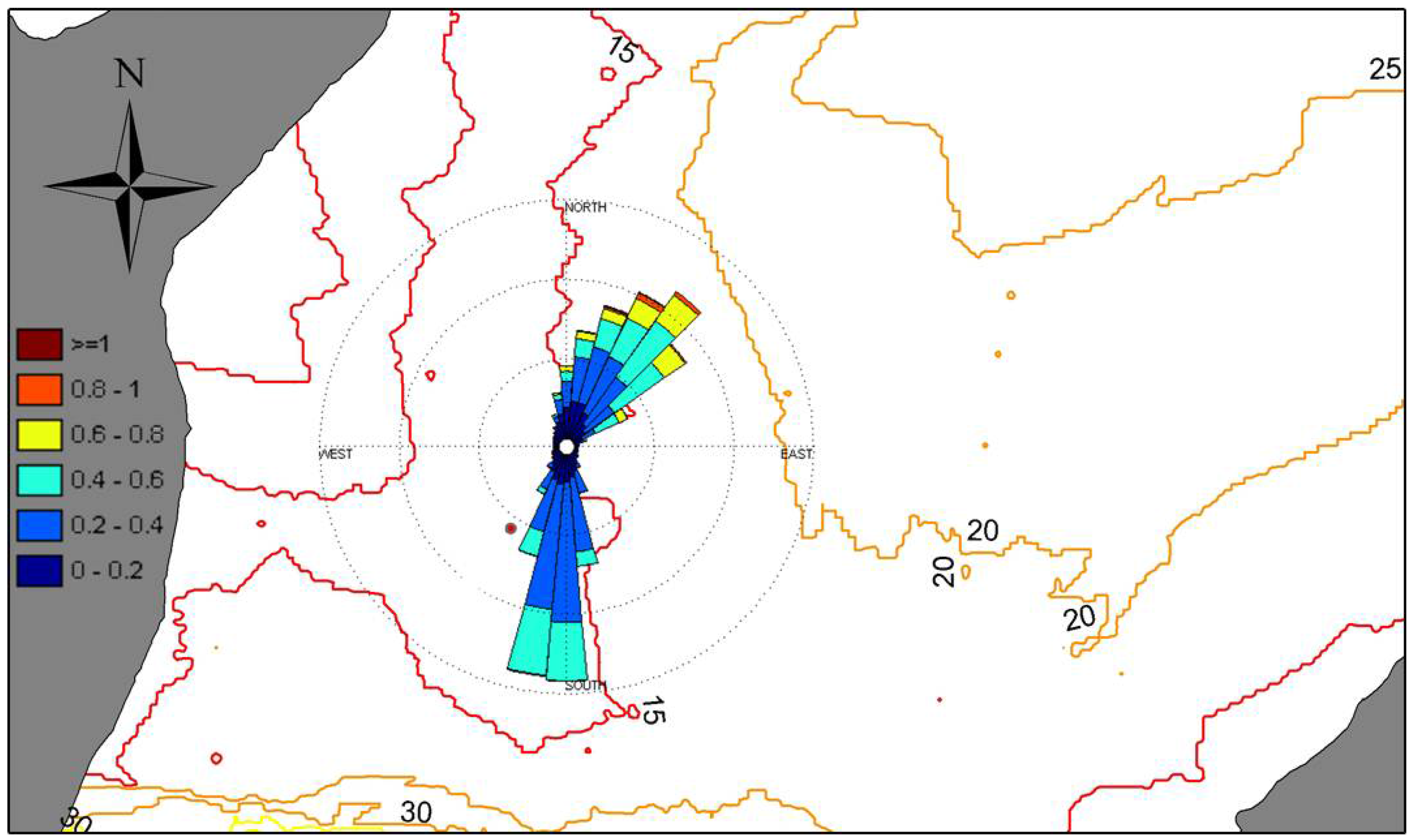
The directions can be seen in Figure 5. The main direction for the flow going out of the fjord is on average N–NE. The spreading of the direction was mostly a result of differences in the vertical layers. For the flow going into the fjord the main direction was S–SW.

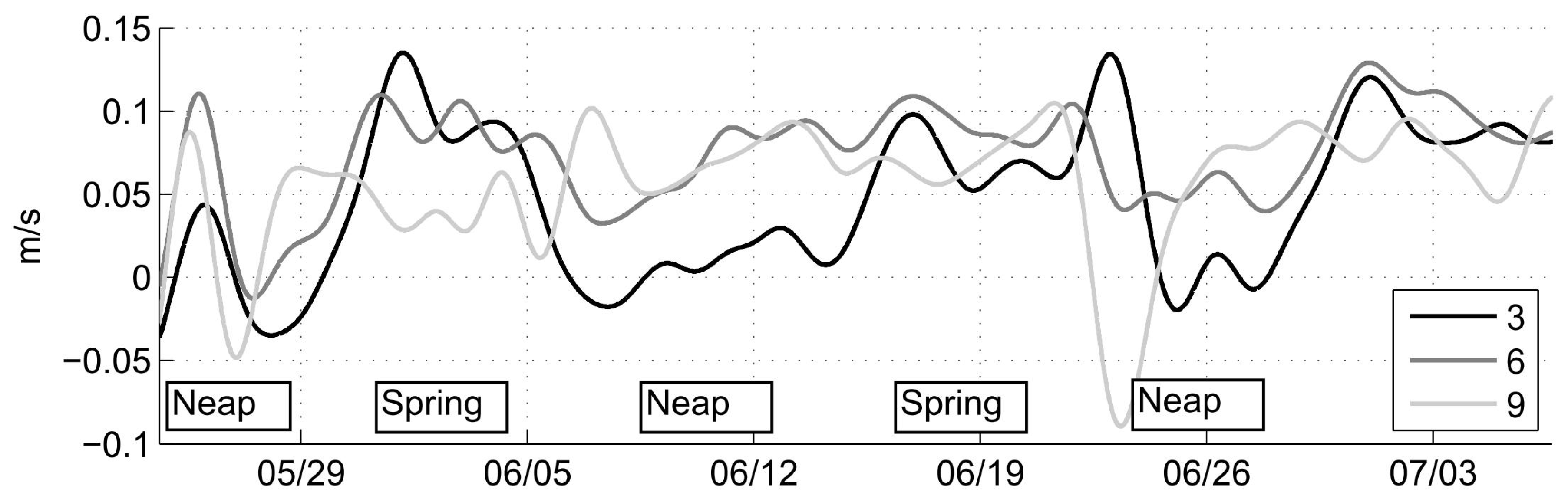
The magnitude of the sustained maximum velocity was almost double for the outgoing tide. The reason for this large difference is probably changed flow paths between in- and outgoing tide, discussed further in Section 4.2. This might not have been observed had the ADCP been placed in the middle of the channel. A Butterworth low-pass filter with a 30 h cut-off frequency was applied on the time-series to remove the influence of the tidal components. The residual current, shown in Figure 6, is caused either by freshwater outflow from the fjord or a differed flow path between ebb and flood in the channel. As seen in the figure, the velocity in the bottom layer and mid-depth layer decreases during neap tide, and increases during spring. The dominant tidal components (semi-diurnal and diurnal) have been removed from the time-series, but a neap-spring relationship is visible. The residual velocity is thus related to the tidal variations, and is not only a cause of the freshwater outflow from the fjord. The change in flow path can thus be a cause of this.

Figure 5. Direction and velocity for the ADCP measurement series. Lengths of bars show incidence of each direction segment and the color bar shows the velocity in m/s.

Figure 5. Direction and velocity for the ADCP measurement series. Lengths of bars show incidence of each direction segment and the color bar shows the velocity in m/s.

Figure 6. Butterworth low-pass filter applied on the time-series of the velocity. Shown is the residual current for the depth 3, 6 and 9 m above the bottom.

Figure 6. Butterworth low-pass filter applied on the time-series of the velocity. Shown is the residual current for the depth 3, 6 and 9 m above the bottom.

The observed higher sustained maximum velocity for the bottom layer compared with layers above is a result of a few occasions (approximately 6 of 84 peaks) where this occurred. In general, the mean velocity for the bottom layer is lower than the depth mean. The frequency of each velocity segment was not taken into account in the calculation of the sustained maximum. However, what causes this increase in velocity for the bottom layer from time to time is unknown.

The tidal level data received from the NHS (observed and predicted) was compared with tidal data measured with the ADCP using its built-in pressure sensor. The results are presented in Table 5 and Figure 7.

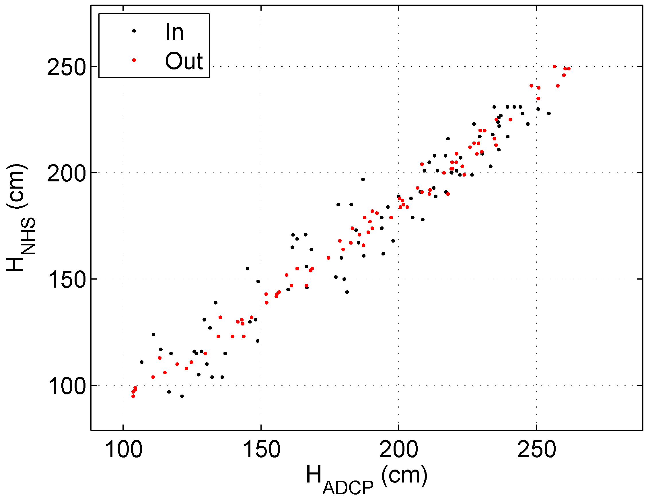
It can be seen that the tidal level data received from the NHS has some discrepancy from the level measured by the ADCP. The NHS values underestimate the measured tidal range by approximately 14 cm. These differences correspond to 7% of the total tidal range. The average of the time lag was 2–3 min, meaning that even though the maximum tidal level occurred at different times between the

Table 5. Difference in tidal range [amplitude difference (amp. diff.)] and time lag between tidal data received from the NHS (observed and predicted) to measured data from the ADCP (measurement #1) in Skarpsundet.

Difference	Predicted (NHS)		Observed (NHS)
	Amp. diff.	Time lag	Amp. diff.	Time lag
Mean	14 cm	2 min	13 cm	3 min
Max	28 cm	20 min	26 cm	40 min
Min	0 cm	−20 min	1 cm	−20 min

Table 5. Difference in tidal range [amplitude difference (amp. diff.)] and time lag between tidal data received from the NHS (observed and predicted) to measured data from the ADCP (measurement #1) in Skarpsundet.

Difference	Predicted (NHS)		Observed (NHS)
	Amp. diff.	Time lag	Amp. diff.	Time lag
Mean	14 cm	2 min	13 cm	3 min
Max	28 cm	20 min	26 cm	40 min
Min	0 cm	−20 min	1 cm	−20 min

Figure 7. Comparison of the calculated tidal range between received data from the NHS and measured ADCP tidal level data. $R^2$ = 99%. Black dots show the flood tidal range, and red dots the ebb tidal range.

Figure 7. Comparison of the calculated tidal range between received data from the NHS and measured ADCP tidal level data. $R^2$ = 99%. Black dots show the flood tidal range, and red dots the ebb tidal range.

NHS and the ADCP, the total effect was on average close to zero. It should be noted that since the data from the NHS is measured every 10 min, a time lag difference of 2–3 min is a result of averages, and not an actual observation.

The correlation is good ($R^2$-value of 99%) between the ADCP-measured and the NHS-predicted tidal value, which is a requirement for further analysis using tidal level data. As seen in Figure 7, the ebb tidal range has less variation than the flood tidal range.

4.2. Cross-Sectional Velocity

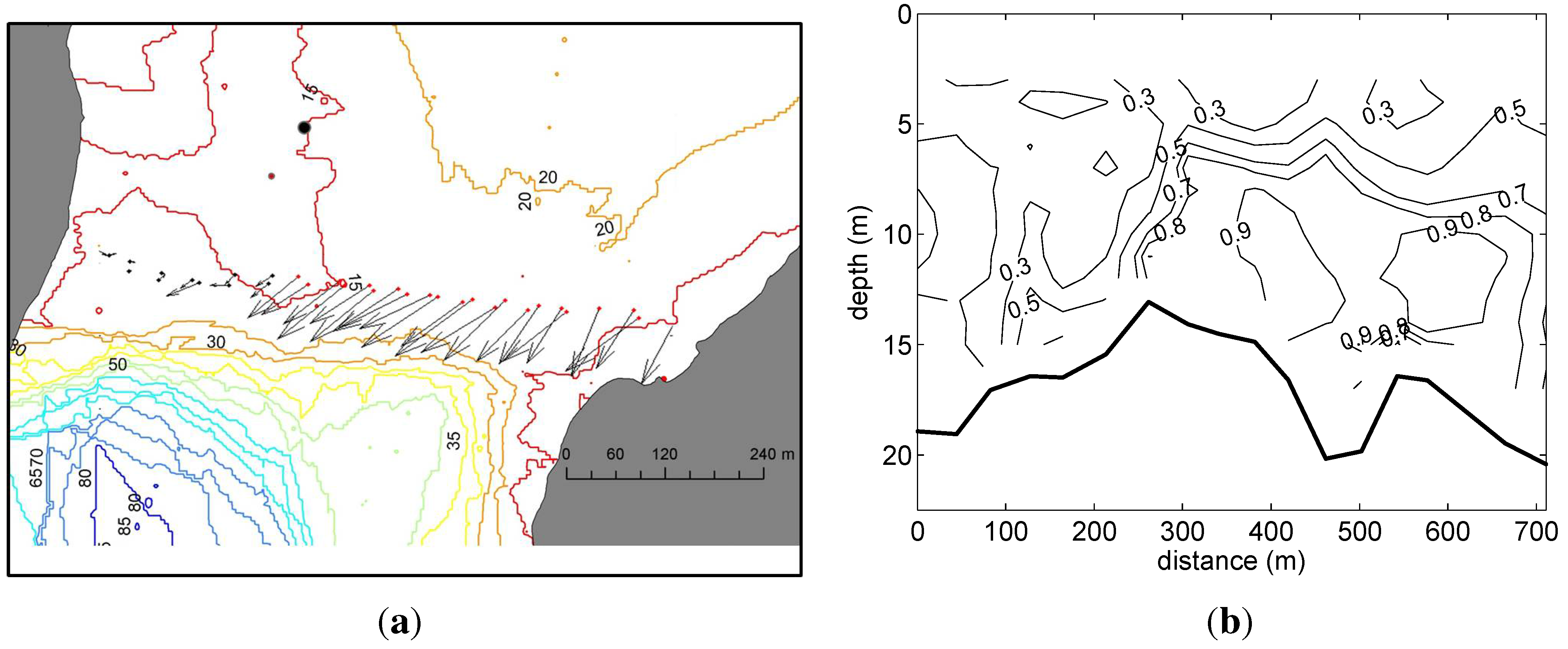
The cross-sectional measurement was only carried out during a rising tide and thus only the velocity field for the incoming tide has been analysed. The tidal level above sea-chart zero was approximately 150 cm during the measurements and the tidal range approximately 200 cm. Since the measurements were carried out 0.5–1.5 h after the estimated time for the highest velocity, the velocities have been scaled assuming a sinusoidal variation to find estimates of the maximum velocity. The cross-sectional average velocity for the two transects was calculated and fitted into a sine curve, yielding a maximum velocity and a time lag for the occurring tide. This correction, adding 1% and 9% to transect measurement 1 and 2 respectively, have been applied in the below calculations.

The result from the two cross-section measurement is shown in Figure 8. The arrows show the depth mean velocity. The average cross-sound velocity was calculated using WinRiver and then scaled, giving a cross-sectional average of 0.4 m/s. In the area of high velocity, from the east bank to the middle of the channel, the scaled depth-averaged velocity was 0.7 m/s.

Figure 8. Results from the cross-sectional measurement. The tide was rising and measurements occurred at 4–5 h after low tide. (a) shows the depth average velocities; and (b) the velocities through the cross-section. Depth is shown in (b) as a thick black line. Cross-sectional average velocity is 0.4 m/s and in 300–700 m in (b) the depth average velocity is 0.7 m/s.

Figure 8. Results from the cross-sectional measurement. The tide was rising and measurements occurred at 4–5 h after low tide. (a) shows the depth average velocities; and (b) the velocities through the cross-section. Depth is shown in (b) as a thick black line. Cross-sectional average velocity is 0.4 m/s and in 300–700 m in (b) the depth average velocity is 0.7 m/s.

From Figure 8, it can be seen that most of the flow during incoming tide is moving at the eastern part of the sound. These results are compared with the TELEMAC simulation and discussed in Section 4.3.

4.3. Simulation Results

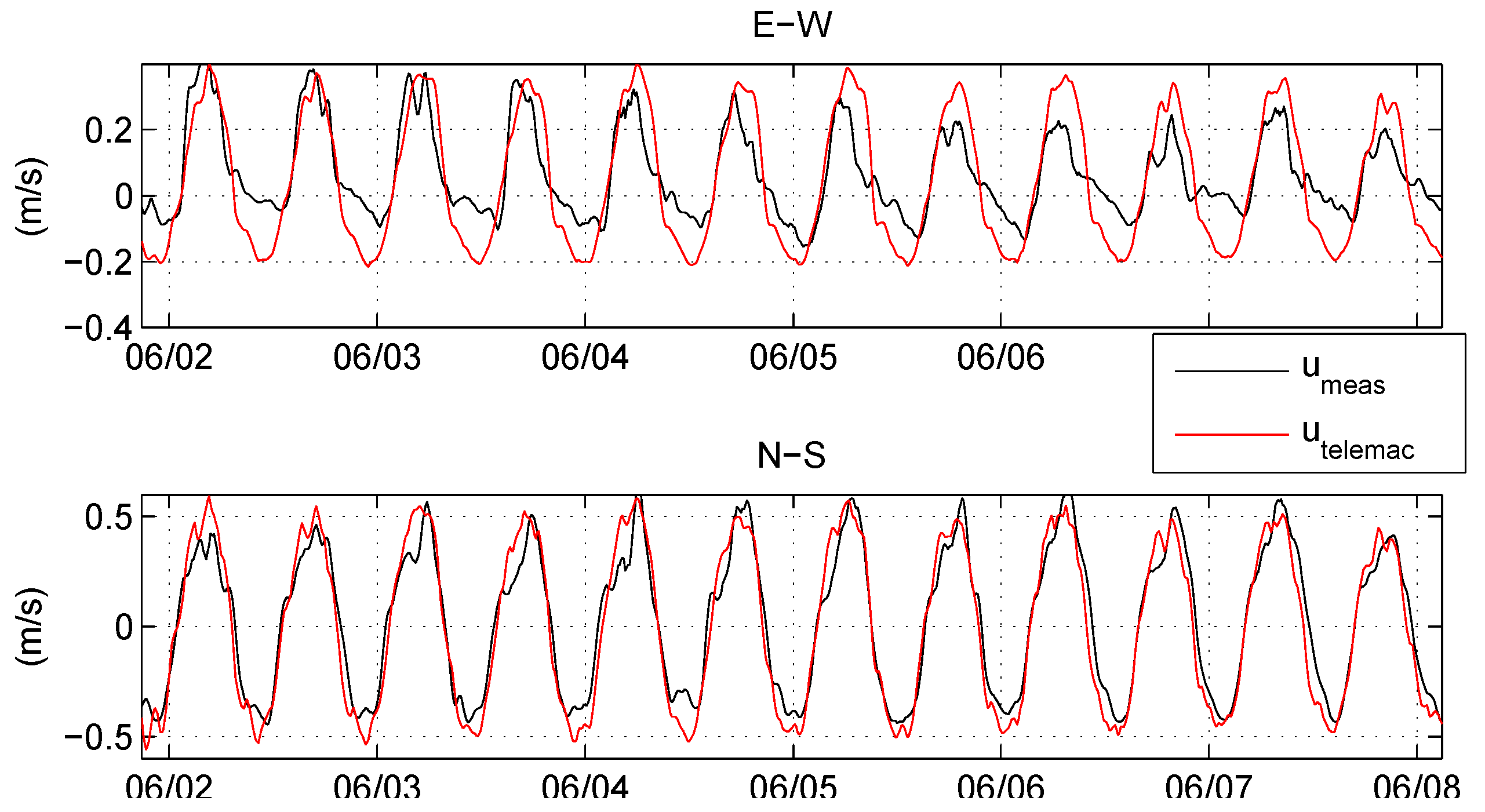
The velocity measured with the ADCP (measurement #1) was compared with the simulated velocities from the TELEMAC-2D simulation output (Figure 9). The N-S velocity component agrees well with the simulated values (Figure 9). The simulated E-W velocity component does not agree well with the measured one, especially not for the incoming tide (negative values). However, for the incoming tide the N-S velocity component is dominant and thus much larger. The measurement results showed this in Figure 5.

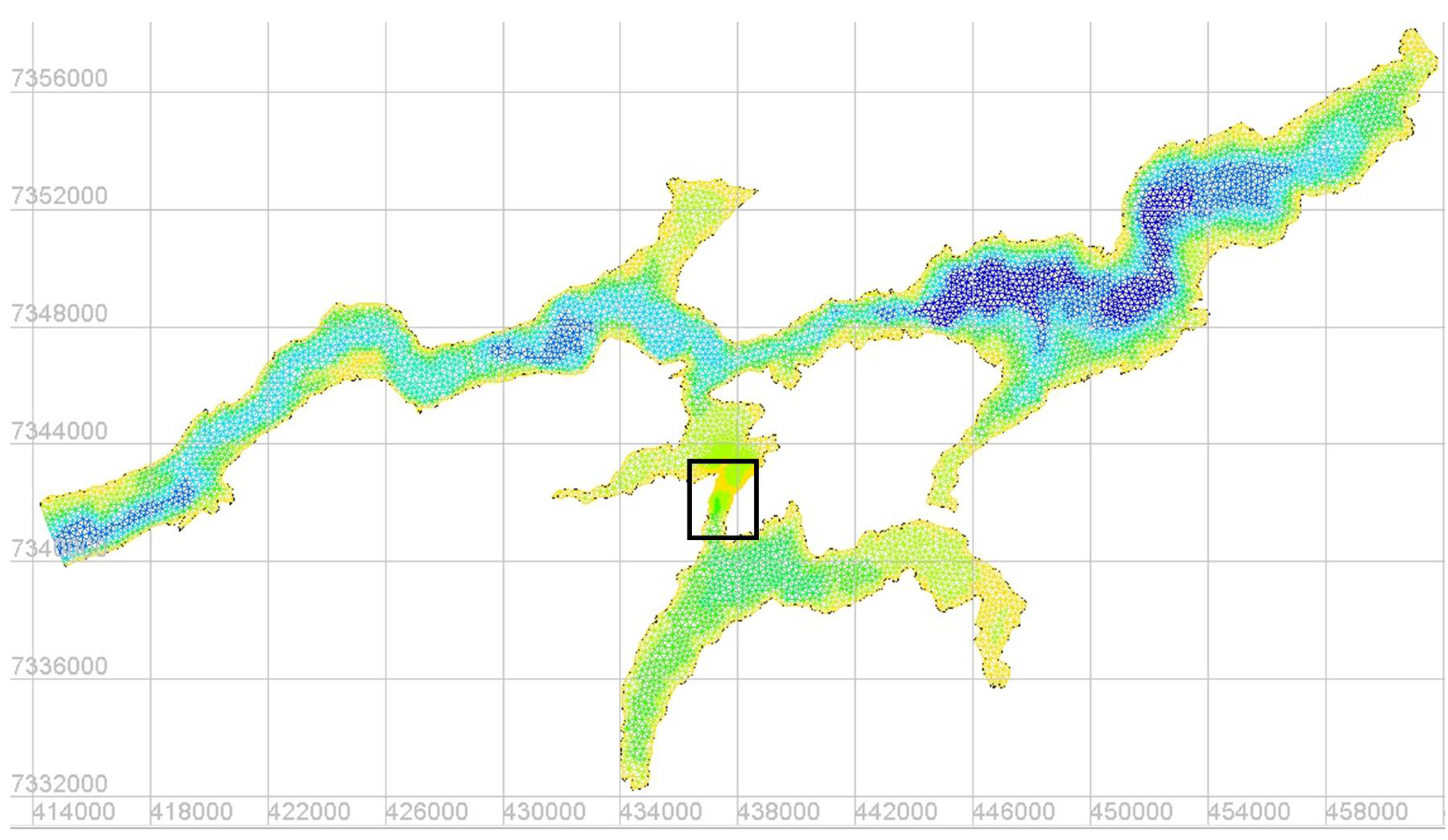
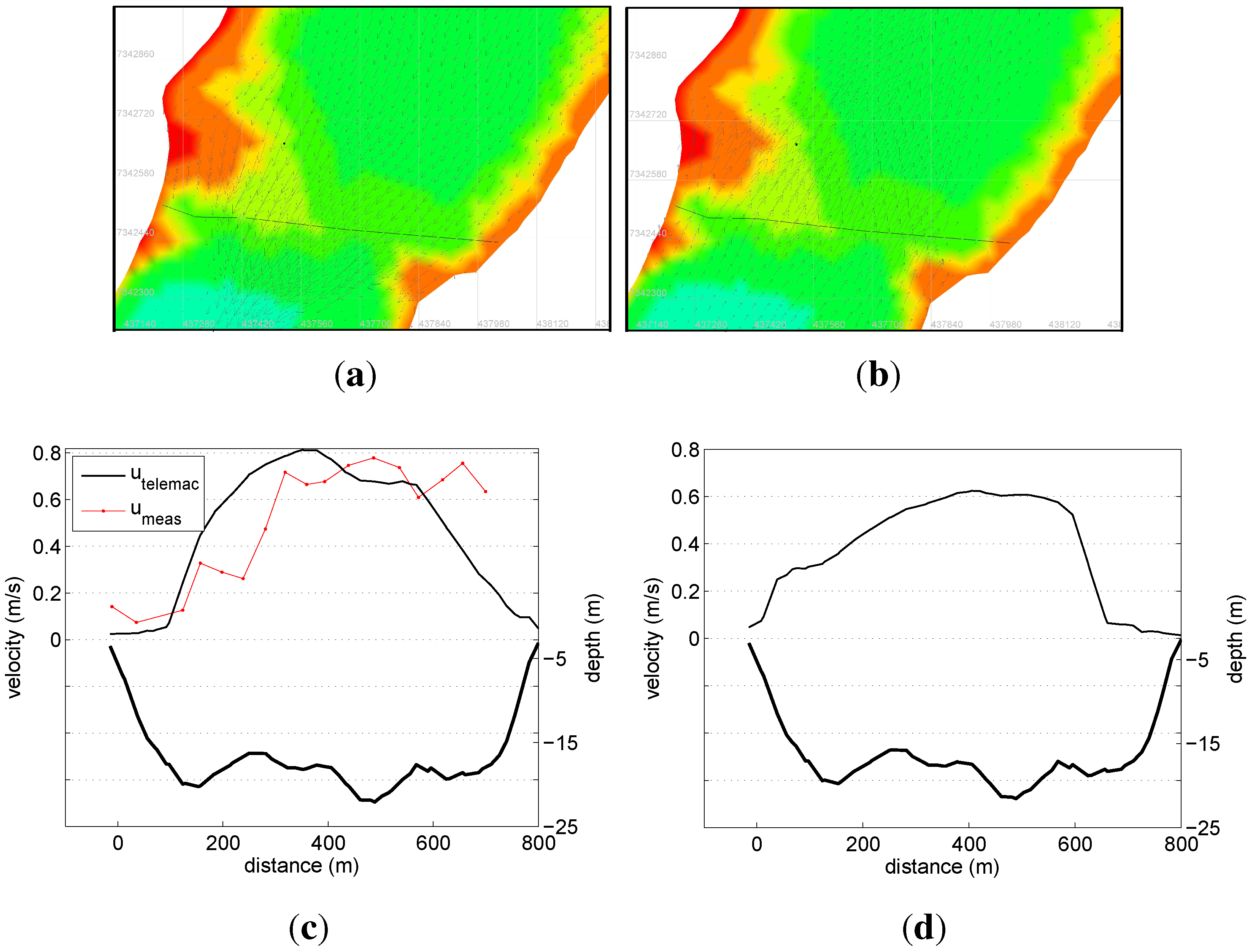
The simulated velocity across the channel is shown in Figure 10. In order for the figures to be comparable with the velocity from the cross-sectional measurement, the plots were taken from a time when the tidal range for the incoming tide was 200 cm. The figure for the outgoing tide (Figure 10b) shows the velocity for the subsequent tide, in which the tidal range was 190 cm. The location of the long-time ADCP measurement is shown with a square as a reference.

Figure 9. Comparison of the E-W and the N-S velocity components between simulated velocity and measured velocity. The simulation was performed with a surface level representing the tide from 1 June to 9 June 2011.

Figure 9. Comparison of the E-W and the N-S velocity components between simulated velocity and measured velocity. The simulation was performed with a surface level representing the tide from 1 June to 9 June 2011.

Figure 10. Velocity field in the sound Skarpsundet modelled with TELEMAC. The tidal range was at the time of the simulation 200 cm (left) and 190 cm (right). Velocity in (a) incoming tide; and (b) outgoing tide is marked with arrows, and the colours represent the bathymetry. The ADCP measurements are marked out where the dot represents the long-time measurement and the line the cross-sectional measurement; (c) Incoming tide profile; and (d) outgoing tide profile show velocity extracted at the same location as the cross-sectional measurement (thin lines) and depth (thick lines). The cross-sectional measurement is plotted in (c) for a comparison.

Figure 10. Velocity field in the sound Skarpsundet modelled with TELEMAC. The tidal range was at the time of the simulation 200 cm (left) and 190 cm (right). Velocity in (a) incoming tide; and (b) outgoing tide is marked with arrows, and the colours represent the bathymetry. The ADCP measurements are marked out where the dot represents the long-time measurement and the line the cross-sectional measurement; (c) Incoming tide profile; and (d) outgoing tide profile show velocity extracted at the same location as the cross-sectional measurement (thin lines) and depth (thick lines). The cross-sectional measurement is plotted in (c) for a comparison.

The cross-sectional average velocity, calculated by dividing the discharge by the cross-sectional area, for the incoming tide in Figure 10c was found to be 0.5 m/s and the highest velocities (at distance 200 to 600 m from the west bank) was 0.7 m/s. The overall average is thus slightly higher than the one measured with the ADCP. However, the velocities were comparable in the centre of the channel. These results confirm that TELEMAC is able to simulate the velocity so that it is comparable with the measurements.

4.4. Evaluation of $\widehat{u}$

Although the purpose was to estimate how well the tidal velocities could be predicted, the investigated site was not ideal as a tidal energy site in terms of the average velocity (see Section 4.1). However, the site was ideal when looking at its location: the only entrance to a fjord with moderate river influence. For the estimation of $\widehat{u}$, the site thus encompasses all requirements.

It is important to repeat that the model gives an estimate of the cross-sectional average velocity. Thus, it does not try to estimate the velocity at any arbitrary location.

4.4.1. Maximum Velocity and Tidal Range

The maximum velocity is according to Equation (7) varying with the tidal range, while the other parameters are constant for each fjord and cross-section. The accuracy of estimating the maximum velocity with the tidal range is analysed in this section. The measured maximum ebb and flood velocity for each tidal cycle was compared with the corresponding tidal range, in order to estimate how well they correlated. For the following section, only the long-time ADCP velocity series have been used. The velocity was depth averaged and smoothed over one hour and only depth 3 to 11 m above the bottom was used. The maximum ebb and flood velocity was then extracted from the time series.

The tidal range has been calculated using the predicted value of the tide obtained from the NHS. The maximum and minimum value was obtained for each tidal cycle. The difference between these was defined as the tidal range. The range from minimum to maximum was compared with the velocity into the fjord and the tidal range from maximum to minimum was compared with the velocity out of the fjord.

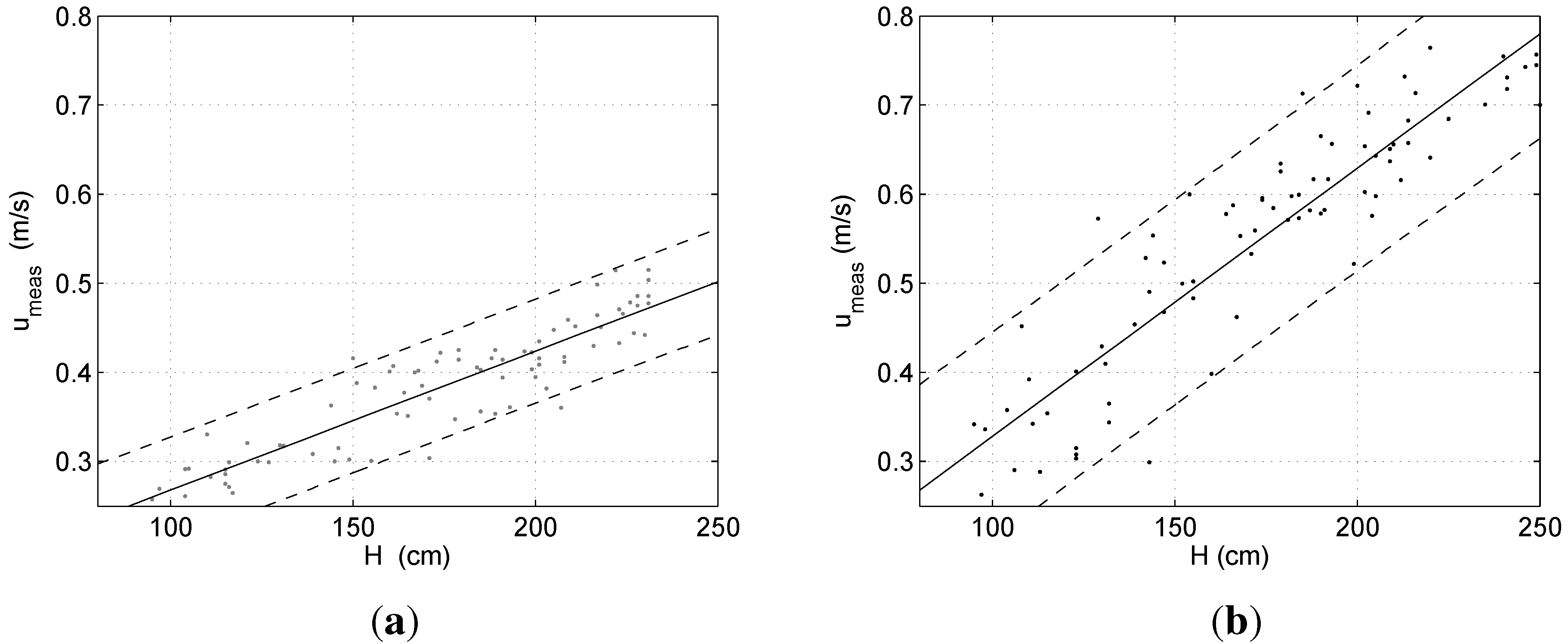
The results from this analysis can be seen in Figure 11 and Table 6. The correlation plot shows that the velocity variation is stronger for the outgoing tide compared with the incoming.

In Table 6 the equation for the straight line in Figure 11 is shown. It can be seen that the slope in the equation is different between the incoming and the outgoing tide, with a higher slope value for the outgoing tide. The maximum velocity occurs on average 3 h and 35 min after high tide and 3 h 32 min after low tide.

Table 6. Parameters for correlating the tidal height with the maximum velocity. $t_{delay}$ is the time in minutes that the maximum velocity will show after high or low tide.

Flow	Variable u	$\text{u}=\text{a}+\mathrm{bH}$	${\text{R}}^2$	${\text{t}}_{\mathrm{delay}}$
Incoming tide	$u_{meas,in}$	$u=0.11m{s}^{-1}+0.16s^{-1}H$	0.83	3h 32min
Outgoing tide	$u_{meas,out}$	$u=0.03m{s}^{-1}+0.30s^{-1}H$	0.84	3h 35min

Table 6. Parameters for correlating the tidal height with the maximum velocity. $t_{delay}$ is the time in minutes that the maximum velocity will show after high or low tide.

Flow	Variable u	$\text{u}=\text{a}+\mathrm{bH}$	${\text{R}}^2$	${\text{t}}_{\mathrm{delay}}$
Incoming tide	$u_{meas,in}$	$u=0.11m{s}^{-1}+0.16s^{-1}H$	0.83	3h 32min
Outgoing tide	$u_{meas,out}$	$u=0.03m{s}^{-1}+0.30s^{-1}H$	0.84	3h 35min

Figure 11. Velocity peaks versus tidal heights: (a) Incoming tide and (b) outgoing tide. Dashed lines show the 95% confidence interval.

Figure 11. Velocity peaks versus tidal heights: (a) Incoming tide and (b) outgoing tide. Dashed lines show the 95% confidence interval.

The velocity for three tidal ranges have been compared in Table 7. The results clearly confirm the asymmetry of the in- and outgoing velocity. For a rising tide the velocity into the fjord is generally lower for the same tidal range and it varies with ± 5 cm/s, whereas with a falling tide the velocity out of the fjord varies with approximately ± 10 cm/s. Note that the results are only valid at the position of the ADCP.

The accuracy of using the tidal range as a variable is not very high, especially not for the outgoing tide. The difference between outgoing and incoming velocity at the position of the long-time measurement is however confirmed by the TELEMAC simulation (Figure 9). Thus, measurements at another location, more centred in the channel, could have yielded different results.

Table 7. Comparing the measured velocity, $u_{meas}$, with the tidal range, H, for spring, mean and neap tide. Index $in$ is incoming velocity (flood) and $out$ is outgoing velocity (ebb). Only maximum values have been compared.

Variable	Tidal range	${\text{u}}_{\mathrm{meas},\mathrm{in}}$	${\text{u}}_{\mathrm{meas},\mathrm{out}}$
	(cm)	(m/s)	(m/s)
$H_{spring}$	224	0.46 ± 0.06	0.70 ± 0.12
$H_{mean}$	166	0.37 ± 0.05	0.53 ± 0.10
$H_{neap}$	109	0.28 ± 0.05	0.36 ± 0.08

Table 7. Comparing the measured velocity, $u_{meas}$, with the tidal range, H, for spring, mean and neap tide. Index $in$ is incoming velocity (flood) and $out$ is outgoing velocity (ebb). Only maximum values have been compared.

Variable	Tidal range	${\text{u}}_{\mathrm{meas},\mathrm{in}}$	${\text{u}}_{\mathrm{meas},\mathrm{out}}$
	(cm)	(m/s)	(m/s)
$H_{spring}$	224	0.46 ± 0.06	0.70 ± 0.12
$H_{mean}$	166	0.37 ± 0.05	0.53 ± 0.10
$H_{neap}$	109	0.28 ± 0.05	0.36 ± 0.08

4.4.2. Modelled and Measured Cross-Sectional Velocity

The estimation of ${\widehat{u}}_{max}$ was performed with values similar as during the cross-sectional measurement. The ADCP transect measurement was performed over a cross-sectional area of 13,500 ${\mathrm{m}}^2\mathrm{a}$nd the tidal range during the measurements was 200 cm. Using Equation (7) with these values, ${\widehat{u}}_{max}$ becomes 0.4 m/s.

This value agrees with the measured cross-sectional average velocity, which was also 0.4 m/s. When comparing with the TELEMAC simulation results (Section 4.3) the average velocity over the transect was 0.5 m/s. This value is also comparable to the estimated $\widehat{u}$.

The model can thus predict the cross-sectional average velocity well. Both the measurement and the simulation, however, showed that the velocity in the centre of the channel was significantly higher than the cross-sectional average. The long-time effect of the difference between the estimated $\widehat{u}$ and the velocity in the centre of the channel is discussed below (Section 4.4.3. ).

4.4.3. Quantification of the Model

The long-time effect of using $\widehat{u}$ to calculate the kinetic energy was quantified by comparing the kinetic energy in the flow at different locations in the channel. This was made possible by using four velocity series from the TELEMAC simulation. Different notations were used depending on the location of the extracted velocity data, but they are referred to as i below. The four different locations that were chosen from the TELEMAC simulation are shown in Figure 12.

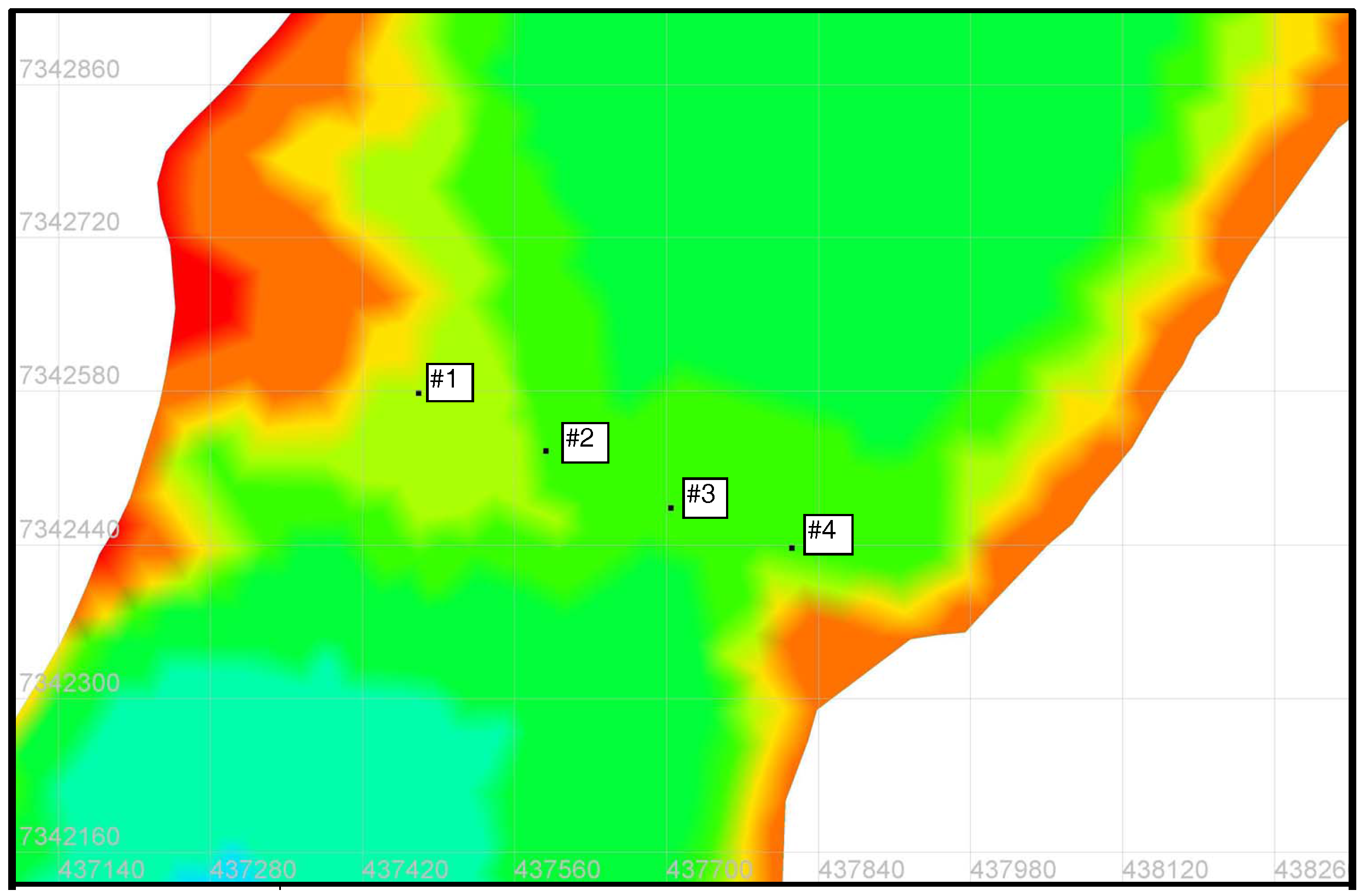
Figure 12. The four selected points that were chosen for quantifying the effect of different velocities in a channel.

Figure 12. The four selected points that were chosen for quantifying the effect of different velocities in a channel.

The kinetic energy in the flow was calculated with Equation (8). The quantification was defined as the percentage difference, $\Delta E_{\%}$, between the kinetic energy calculated using the TELEMAC simulated velocity ($E_{telemac,i}$) and the estimated velocity ($\widehat{E}$):

$$\Delta E_{\%}=\frac{E_{telemac,i}-\widehat{E}}{\overline{\widehat{E}}}·100$$

(12)

The average daily difference was estimated with Equation (12) using accumulated daily values of $E_{telemac,i}$ and $\widehat{E}$. The average daily difference of $\Delta E_{\%}$ is presented in Table 8. The total difference was also estimated with Equation (12), but then $E_{telemac,i}$ and $\widehat{E}$ were total accumulated values at the end of the 14 day series.

Table 8. Result of calculations of $\Delta E$ for 14 days. $E_{telemac,i}$ is calculated with velocity data from the TELEMAC simulation, extracted from four different positions in the channel. Positive values indicate that $E_{telemac,i}$ is higher than $\widehat{E}$.

#	Average daily $\Delta {\text{E}}_{\%}$	Total $\Delta {\text{E}}_{\%}$
# 1	143	202
# 2	200	270
# 3	167	236
# 4	75	118

Table 8. Result of calculations of $\Delta E$ for 14 days. $E_{telemac,i}$ is calculated with velocity data from the TELEMAC simulation, extracted from four different positions in the channel. Positive values indicate that $E_{telemac,i}$ is higher than $\widehat{E}$.

#	Average daily $\Delta {\text{E}}_{\%}$	Total $\Delta {\text{E}}_{\%}$
# 1	143	202
# 2	200	270
# 3	167	236
# 4	75	118

Table 8 shows the percentage difference between a tidal velocity series created entirely with publicly available data versus results from the TELEMAC simulation. The model used for creating $\widehat{u}$, and consequently $\widehat{E}$, can only be used to calculate the cross-sectional average. The total difference in kinetic energy between $\widehat{u}$ and $u_{telemac,i}$ indicate how large the error would be if $\widehat{u}$ was the sole parameter used for estimating the tidal resource in the sound. 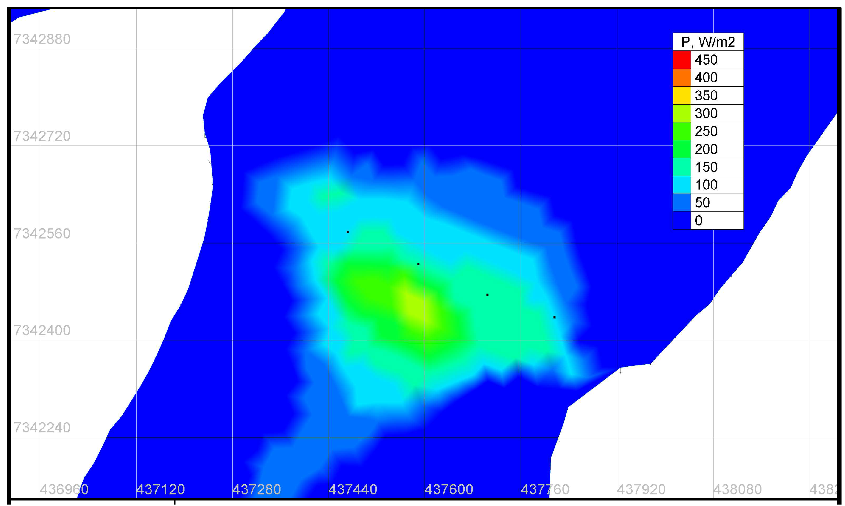In Figure 13, the distribution of the cube of the velocity is shown and it can be seen that the resource intensity is much larger in the centre of the channel.

Figure 13. Example of the resource distribution ($P_{telemac}/m^2$) for an incoming tide (same time as Figure 10a). Black dots are the four selected points chosen for quantifying the effect of different cross-sectional velocities (Figure 12). The incoming tidal resource is higher in the centre of the channel.

Figure 13. Example of the resource distribution ($P_{telemac}/m^2$) for an incoming tide (same time as Figure 10a). Black dots are the four selected points chosen for quantifying the effect of different cross-sectional velocities (Figure 12). The incoming tidal resource is higher in the centre of the channel.

The results show that the underestimation of the velocity will have the consequence of a large underestimation of the resource. The model we have analysed so far does not appear to be suitable to calculate the kinetic energy of the flow. However, the intention of calculating $\widehat{u}$ was to estimate the magnitude of the maximum velocity, in order to find sites where in-depth measurements may be of interest. Thus, as a first screening tool, the model is considered viable.

4.5. Calculation of ${\widehat{u}}_{max}$ in other fjords

The ${\widehat{u}}_{max}$ (Section 3.1) was calculated in several of the sites presented by Grabbe et al. [1]. Of the more than 100 listed sites, a total number of 31 sites were regarded as suitable for the presented model, i.e., the sites connected a bay to the open ocean. Due to poor depth data at some of the sites, only 15 of these were chosen to perform the calculations. The velocities were calculated using the maximum spring tidal range, $H_{spring}$, and the cross-sectional area was calculated by including half the tidal range. The results are presented in Table 9.

Table 9. Velocity data taken from the Norwegian Pilot book ($u_p$) and transformed by Grabbe et al. [1] compared with modelled velocity ($\widehat{u})$ using the model described in Section 3.1. $\widehat{u}$ has been calculated using the mean spring tidal range. Due to the site Skarpsundet not being mentioned in the Norwegian pilot books it has been labelled with number 0. The choking factor has been calculated using a channel length of 1000 m and the values shown in the table.

No.	Fjord name	Latitud	Longitud	${\text{A}}_{\text{c}}$bl	${\text{A}}_{\text{f}}$bl	${\text{H}}_{\mathrm{spring}}$	${\text{u}}_{\text{p}}$	${\widehat{\text{u}}}_{\max }$	Choking
				(${\text{m}}^2$)	(${\mathrm{km}}^2$)	(m)	(m/s)	(m/s)	(%)
0	Skarps., Hemnesb.	${66}^{\circ }{11}^{\prime }$	${13}^{\circ }{36}^{\prime }$	13,500	38	2.24	–	0.44	0
1	Bakkestr., Nords.	${64}^{\circ }{55}^{\prime }$	${11}^{\circ }{29}^{\prime }$	320	7	2.12	3.1	3.4	47
2	Messemstr., Nords.	${64}^{\circ }{54}^{\prime }$	${11}^{\circ }{31}^{\prime }$	950	6	2.12	0.8	0.90	0.4
3	Nordfj., Rødøy	${66}^{\circ }{36}^{\prime }$	${13}^{\circ }{33}^{\prime }$	14,220	10	2.24	2.1	0.10	0
4	Kjellings., Beiarfj.	${67}^{\circ }{05}^{\prime }$	${14}^{\circ }{19}^{\prime }$	1,300	2	2.24	2.1	0.22	0
5	Graddstraumen	${67}^{\circ }{14}^{\prime }$	${15}^{\circ }{00}^{\prime }$	1,270	22	2.24	3.1	2.8	43
6	Straumen, Rombaksb.	${68}^{\circ }{26}^{\prime }$	${17}^{\circ }{42}^{\prime }$	4,700	7	2.70	2.1	0.29	0
7	Ytterpollen, Tysfjord	${68}^{\circ }{05}^{\prime }$	${16}^{\circ }{41}^{\prime }$	610	1	2.51	2.1	0.32	0
8	Straumbotn, Ibestad	${68}^{\circ }{55}^{\prime }$	${17}^{\circ }{11}^{\prime }$	130	7	1.88	5.1	7.1	87
9	Grovfjorden	${68}^{\circ }{40}^{\prime }$	${17}^{\circ }{07}^{\prime }$	430	7	1.88	2.1	2.1	46
10	Godfj., Kvæfjord	${68}^{\circ }{45}^{\prime }$	${15}^{\circ }{50}^{\prime }$	1,460	2	1.88	2.1	0.2	0
11	Skarmunken, Tromsø	${69}^{\circ }{36}^{\prime }$	${19}^{\circ }{43}^{\prime }$	4,170	57	2.24	1.5	2.1	13
12	Storstr., Kvænang.	${69}^{\circ }{50}^{\prime }$	${21}^{\circ }{53}^{\prime }$	1,290	31	2.24	2.6	3.8	55
13	Lillestr., Kvænang.	${69}^{\circ }{46}^{\prime }$	${22}^{\circ }{02}^{\prime }$	1,970	14	2.24	1.5	1.1	5
14	Straumen, Kåfjorden	${69}^{\circ }{56}^{\prime }$	${23}^{\circ }{03}^{\prime }$	490	2	2.32	3.1	0.68	1
15	Straumen, Kongsfj.	${70}^{\circ }{42}^{\prime }$	${29}^{\circ }{23}^{\prime }$	520	10	2.70	3.1	3.5	51

Table 9. Velocity data taken from the Norwegian Pilot book ($u_p$) and transformed by Grabbe et al. [1] compared with modelled velocity ($\widehat{u})$ using the model described in Section 3.1. $\widehat{u}$ has been calculated using the mean spring tidal range. Due to the site Skarpsundet not being mentioned in the Norwegian pilot books it has been labelled with number 0. The choking factor has been calculated using a channel length of 1000 m and the values shown in the table.

No.	Fjord name	Latitud	Longitud	${\text{A}}_{\text{c}}$bl	${\text{A}}_{\text{f}}$bl	${\text{H}}_{\mathrm{spring}}$	${\text{u}}_{\text{p}}$	${\widehat{\text{u}}}_{\max }$	Choking
				(${\text{m}}^2$)	(${\mathrm{km}}^2$)	(m)	(m/s)	(m/s)	(%)
0	Skarps., Hemnesb.	${66}^{\circ }{11}^{\prime }$	${13}^{\circ }{36}^{\prime }$	13,500	38	2.24	–	0.44	0
1	Bakkestr., Nords.	${64}^{\circ }{55}^{\prime }$	${11}^{\circ }{29}^{\prime }$	320	7	2.12	3.1	3.4	47
2	Messemstr., Nords.	${64}^{\circ }{54}^{\prime }$	${11}^{\circ }{31}^{\prime }$	950	6	2.12	0.8	0.90	0.4
3	Nordfj., Rødøy	${66}^{\circ }{36}^{\prime }$	${13}^{\circ }{33}^{\prime }$	14,220	10	2.24	2.1	0.10	0
4	Kjellings., Beiarfj.	${67}^{\circ }{05}^{\prime }$	${14}^{\circ }{19}^{\prime }$	1,300	2	2.24	2.1	0.22	0
5	Graddstraumen	${67}^{\circ }{14}^{\prime }$	${15}^{\circ }{00}^{\prime }$	1,270	22	2.24	3.1	2.8	43
6	Straumen, Rombaksb.	${68}^{\circ }{26}^{\prime }$	${17}^{\circ }{42}^{\prime }$	4,700	7	2.70	2.1	0.29	0
7	Ytterpollen, Tysfjord	${68}^{\circ }{05}^{\prime }$	${16}^{\circ }{41}^{\prime }$	610	1	2.51	2.1	0.32	0
8	Straumbotn, Ibestad	${68}^{\circ }{55}^{\prime }$	${17}^{\circ }{11}^{\prime }$	130	7	1.88	5.1	7.1	87
9	Grovfjorden	${68}^{\circ }{40}^{\prime }$	${17}^{\circ }{07}^{\prime }$	430	7	1.88	2.1	2.1	46
10	Godfj., Kvæfjord	${68}^{\circ }{45}^{\prime }$	${15}^{\circ }{50}^{\prime }$	1,460	2	1.88	2.1	0.2	0
11	Skarmunken, Tromsø	${69}^{\circ }{36}^{\prime }$	${19}^{\circ }{43}^{\prime }$	4,170	57	2.24	1.5	2.1	13
12	Storstr., Kvænang.	${69}^{\circ }{50}^{\prime }$	${21}^{\circ }{53}^{\prime }$	1,290	31	2.24	2.6	3.8	55
13	Lillestr., Kvænang.	${69}^{\circ }{46}^{\prime }$	${22}^{\circ }{02}^{\prime }$	1,970	14	2.24	1.5	1.1	5
14	Straumen, Kåfjorden	${69}^{\circ }{56}^{\prime }$	${23}^{\circ }{03}^{\prime }$	490	2	2.32	3.1	0.68	1
15	Straumen, Kongsfj.	${70}^{\circ }{42}^{\prime }$	${29}^{\circ }{23}^{\prime }$	520	10	2.70	3.1	3.5	51

First of all it should be noted that the velocities described by Grabbe et al. [1] are derived from the Norwegian Pilot books (NP). There are very few velocity measurements in fjord openings in Norway and mostly the velocities in the NP are denoted as strong or difficult to pass. Grabbe et al. [1] converted the velocities from texts such as “strong” to a number using a conversion table that had been received from the authors of the NP. The velocities presented in [1], $u_p$, are thus rather uncertain. Nonetheless, the statements in the pilot book give an indication as to whether or not strong currents exist. For instance, Skarpsundet is not mentioned in the NP and indeed it is a site with moderate tidal influence.

We have not attempted to calculate the kinetic energy at each of the sites, since the results shown in Section 4.4.3. concluded that $\widehat{u}$ will give large errors in the kinetic energy calculation. Thus the results of this section are presented with the aim of finding sites where further analysis can be made.

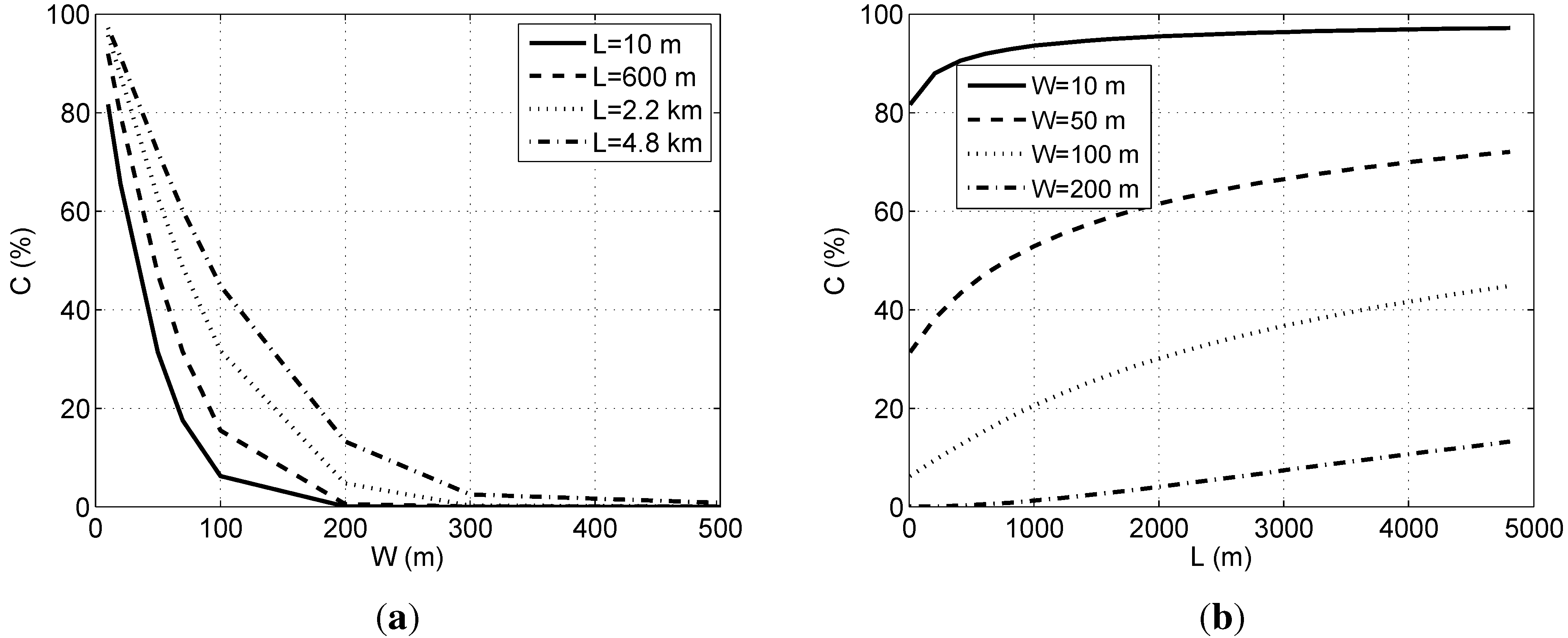
The choking factor in Table 9 has been calculated for all sites to see where ${\widehat{u}}_{max}$ can be used. As mentioned in Section 3.1, the estimation of $\widehat{u}$ can only be made in channels where the friction and acceleration term in the momentum balance can be ignored [15]. For choking factors larger than a few percent, $\widehat{u}$ will overestimate the velocity. Thus, the maximum velocity for a few of the sites will show inflated values (#1, 5, 8, 9, 11, 12, 15).

The velocity $u_p$ was close to ${\widehat{u}}_{max}$ for many of the sites (# 1, 2, 5, 9, 11, 12, 13, 15). As mentioned, the velocity in channels where choking is important will be lower than mentioned in the table. Since $u_p$ is comparable to ${\widehat{u}}_{max}$ for the sites where choking is important, it is likely that $u_p$ also is inflated.

The velocity in the remaining sites differed strongly. As can be seen in site # 8 the calculated value is far higher than the one noted in the NP, probably a result of assuming negligible friction. There are also sites where the calculated velocity is far lower than what is claimed in the NP. There can be many reasons for this, but most likely it is due to misinterpretation of the denoted velocity in the NP. Since $\widehat{u}$ is only the cross-sectional average velocity, many of these site are likely to have higher velocities in the centre of the channel. Our analysis showed that the velocity in the centre can be as much as twice as high as ${\widehat{u}}_{max}$. Thus, why $u_p$ is denoted as 10 times as high as our calculation of ${\widehat{u}}_{max}$ is hard to say without further analysis of each of the regarded sites (#3, 4, 6, 7).

A few sites seem more promising than others, such as site # 2, 5, 11, 12, 13 and 15, due to both a high velocity and a fairly large cross-sectional area. However, since # 5, 12, 15 have choking factors close to 50%, all are likely to have inflated values of ${\widehat{u}}_{max}$ and a more sophisticated model would have to be used to calculate the cross-sectional average maximum velocity.

5. Conclusions

The main purpose of the paper was to present and evaluate a model for estimating the velocity in fjord entrances. The applied model can be regarded as a simple and low-cost tool for estimating the velocity, as it only requires publicly available data to use.

It was shown that using the tidal range as a value for estimating the maximum velocity will have quite low accuracy. However, it was discussed whether this was a result of the chosen location for the long-time measurement. The variation was larger depending on whether the tide was going out or in. Further analysis with the ADCP at a more centralised location would have to be made.

The estimated value of the maximum velocity, ${\widehat{u}}_{max}$, was shown to agree well with the cross-sectional average velocity. However, in the centre of the channel the measured maximum velocity was shown to be higher with almost 100%. In the long-run, an underestimation of the velocity in the sound will have large consequences on the kinetic energy in the flow. Thus, this was quantified by calculating the kinetic energy in the channel per unit area both using the time-series $\widehat{u}$ and velocity data extracted from the TELEMAC simulation. The results showed that the method for estimating $\widehat{u}$ was not accurate enough to calculate the kinetic energy in the flow, since it is dependent on the cube of the velocity. Even at locations that were not in the centre of the channel, $\widehat{u}$ will overestimate the resource. Thus, the model should only be applied to find sites that may be of interest for further analyses.

The calculation of $\widehat{u}$ was performed for several fjord entrances reported in [1]. The results were compared with the velocity values in the Norwegian Pilot Book. For many of the sites studied the velocity agreed with the values in the pilot books, but for some sites the results differed strongly. Further analysis on these sites is required to define why such large differences exist. The model can be summarised as a good screening tool for finding interesting tidal energy resource sites, but not to be used for estimating the tidal energy resource.