The Influence of Output Variability from Renewable Electricity Generation on Net Energy Calculations

Abstract
: One key approach to analyzing the feasibility of energy extraction and generation technologies is to understand the net energy they contribute to society. These analyses most commonly focus on a simple comparison of a source's expected energy outputs to the required energy inputs, measured in the form of energy return on investment (EROI). What is not typically factored into net energy analysis is the influence of output variability. This omission ignores a key attribute of biological organisms and societies alike: the preference for stable returns with low dispersion versus equivalent returns that are intermittent or variable. This biologic predilection for stability, observed and refined in academic financial literature, has a direct relationship to many new energy technologies whose outputs are much more variable than traditional energy sources. We investigate the impact of variability on net energy metrics and develop a theoretical framework to evaluate energy systems based on existing financial and biological risk models. We then illustrate the impact of variability on nominal energy return using representative technologies in electricity generation, with a more detailed analysis on wind power, where intermittence and stochastic availability of hard-to-store electricity will be factored into theoretical returns.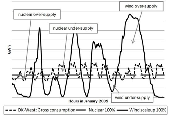
1. Introduction
Besides perhaps water, energy is the most important contributor to life on our planet. Over time, natural selection has optimized towards the most efficient methods for energy capture, transformation, and consumption [1–3]. In order to survive, each organism needs to procure at least the amount of energy it consumes. For example, cheetahs that repeatedly expend more energy chasing a gazelle than they receive from eating it will not survive. Further, in order for body maintenance and repair, reproduction, and the raising of offspring, the cheetah will need to obtain significantly more calories from its prey than it expends chasing it. This amount of energy left over after the calories used to locate, harvest (kill), refine and utilize the original energy are accounted for is termed “net energy”. In the human sphere, this same concept applies. Energy sources need to return more energy than used in their retrieval, and in order to secure an average modern human lifestyle including shelter, amenities, leisure activities and many more benefits beyond the bare necessities, such an energy surplus needs to be significant [4].
Human history has been one of transitions in energy quantity and quality. The value of any energy transformation process to society is proportional to the amount of surplus energy it can produce in excess of what it needs for self-replication [5]. Over time, our trajectory from using sources like biomass and draft animals, to wind and water power, to fossil fuels and electricity has enabled large increases in per capita output because of increases in the quantity of fuels available to produce non-energy goods. This transition to higher energy gain fuels also enabled social and economic diversification as less of our available energy was needed for the energy securing process itself, thereby diverting more energy towards non-extractive activities [6].
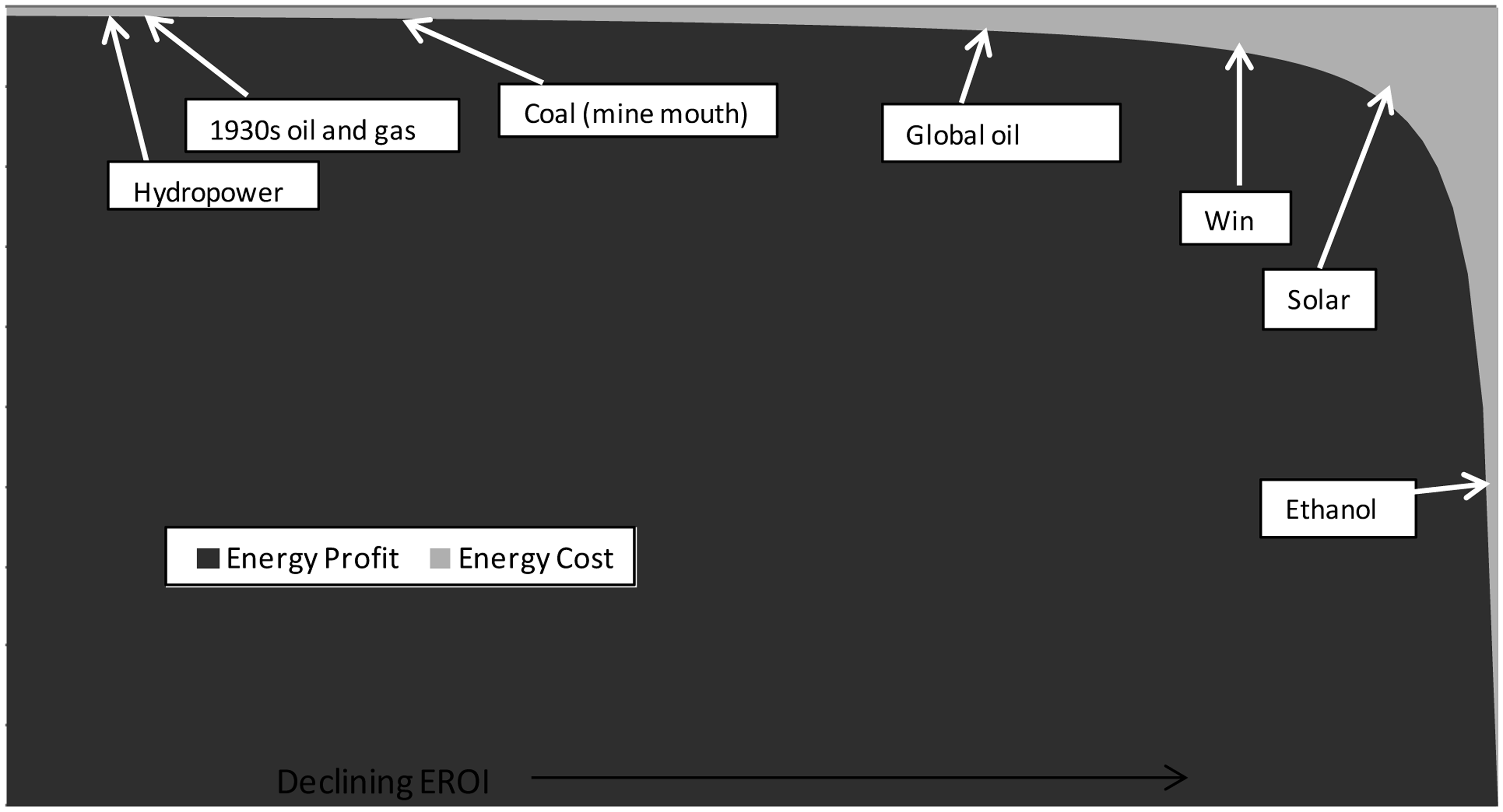
As fossil fuels become more difficult to retrieve and thus more expensive, a move from higher to lower energy gain fuels will have important implications for both how our societies are powered, and structured. As illustrated in Figure 1, declines in aggregate Energy Return on Energy Invested (EROI) mean more energy will be required by the energy sector (the light gray) leaving less energy available for other areas of an economy (the dark gray). Declines in amounts of surplus energy have been linked to collapses of animal societies and historical human civilizations [7]. Research into precisely how much net energy we might need to sustain human civilization is an interesting and important question, but one not frequently addressed [3].
In the past few decades, a number of concepts have been introduced to measure this relationship between energy input and energy gains for energy sources, for example energy profit ratio, EROI, energy payback period, net energy, and energy yield. These biophysical statistics always describe the amount of energy procured for human use relative to the amount expended. Every energy system incurs initial energy expenditures during its own construction. The facility then produces an energy output for a number of years until the end of its effective lifetime is reached. Over time, additional energy costs are incurred in the operation and maintenance of the facility. The simplest statistic to measure these energy flows is “energy gain”, which is the sum of the total energy output less the sum of the total energy input over the life of the investment. A variation of this is EROI, which divides the total energy output by the energy input to arrive at a ratio, indicative of the energy harnessing return potential of the particular technology (Table 1). EROI is sometimes also referred to as the “Energy Profit Ratio”. Another popular statistic is the “energy payback period”, which is the time it takes an energy procuring technology to “pay back” or produce an amount of energy equivalent to that invested in its construction. This method is limited in that it does not account for the total remaining energy output after the initial “payback period”, which might differ significantly for technologies with the same pay-back time. In this paper, we will use the output/input ratio EROI, though the concepts presented here will be applicable to any biophysical statistic measuring net energy.
Net energy is central to an energy theory of value which asserts that natural resources, particularly energy, as opposed to dollars, are what we have to budget and spend [10]. This mode of analysis was viewed as so fundamental that in 1974 the U.S. Congress required every government sponsored technology for procuring energy to be subject to net energy analysis. Net energy analysis, though popular during the energy crises of the 1970s had largely been subsumed in the academic literature by Life Cycle Assessment, until a recent resurgence in biophysical analysis in the last few years sparked by concerns about oil depletion [3].
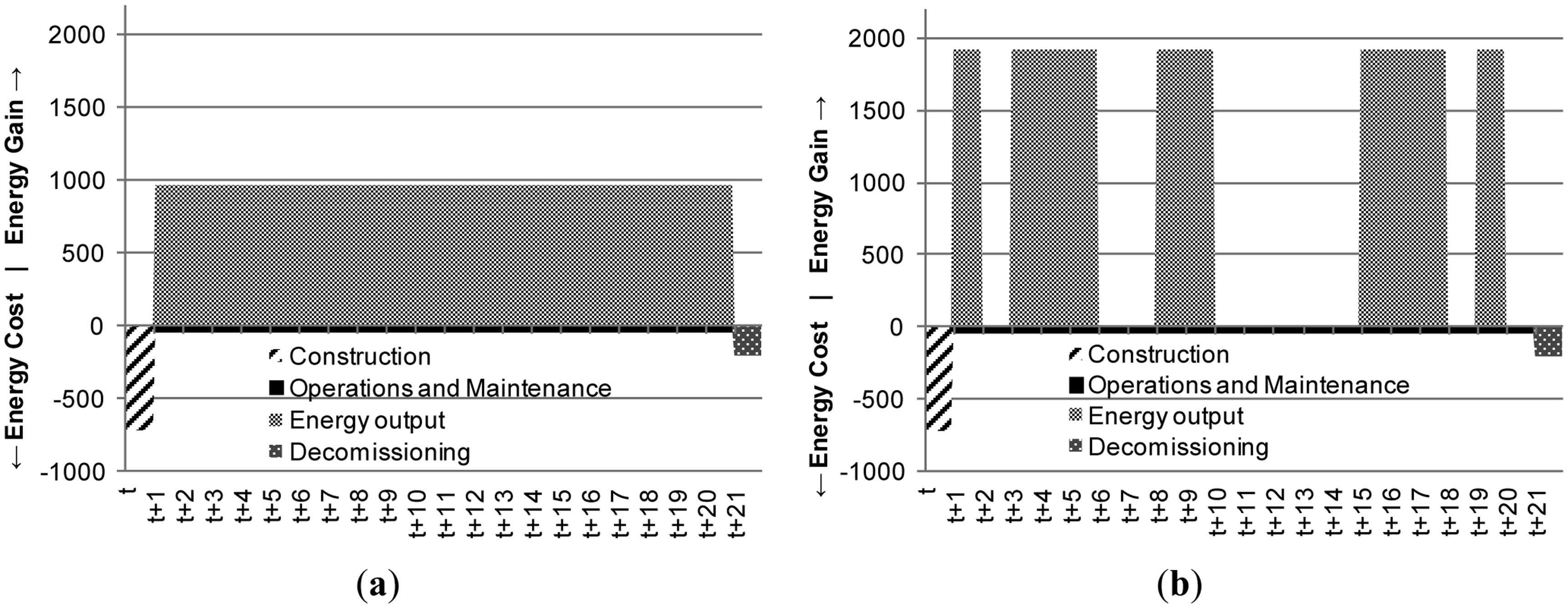
EROI in the studies above and others, is represented as a static integer representing the ratio of energy output to energy expense for the life of an energy technology. This graphically can be represented using an energy flow diagram (Figure 2a). The gray shaded region represents the energy output beginning at time t + c (where c is the period required for construction of facilities) and ending at time t + e (where e is the total number of years with energy gains). The black diagonally-striped section (bottom left) is the initial energy investment needed from the beginning of an energy gathering project. The black section represents ongoing inputs in energy terms through time t + e. Depending on the boundaries, there may also be another energy expense at time T…T + n dealing with decommissioning and waste removal (black dotted section, bottom right).
In traditional net energy analysis, an energy input or output is treated the same irrespective of the volatility stream of the underlying energy output. However, the operational requirements for electrical grids have considerable influence on our energy preferences and planning decisions. Even though 100 continuous kilowatt hours of electricity has the same energy content as 100 sporadically generated kilowatt hours, their usefulness and value is proportionate to their fit with human demand systems. As such, volatility and intermittency become important variables. Variability will refer to a measure of statistical dispersion, either referring to the variance (describing how far measured values lie from the mean) or standard deviation (the square root of the variance). In finance, variability is usually termed “volatility”. Intermittency refers to the non-continuous, stochastic nature of electricity generation by some sources. A stochastic process is one that is random, or non-deterministic.
The two hypothetical graphs for energy retrieval illustrate the relevance of variability (Figure 2). Both of the technologies offer the same EROI but the system in Figure 2a returns energy steadily over 20 periods while the system in Figure 2b returns double the energy and zero energy in random periods. The energy costs are identical at the start and during the life of the asset. Provided the quality of the energy retrieved is comparable, societies would prefer the technology that delivers the more stable returns (the graph on the left), as this more closely matches demand. However, nominal EROI analyses treat these two sources as equally preferable.
Risk, a fundamental feature of our natural environment, is typically defined as variance around a mean, although other definitions include the coefficient of variation, and unanticipated volatility [18,19]. Risk is generally considered as “the effect of uncertainty on objectives” [20]. Greater variability is associated with higher risk because it increases the chances for unknown outcomes and consequences.. Variability risk is a significant aspect of decision-making in both the animal and human world [21,22]. Using a simple example may illustrate the problem with variability from a biological perspective. A pride of lions travels a large distance to a water hole where for years they have found gazelles to feed on. At one point, however, they find the water hole dried up, with no prey (and no water) available. Despite the fact that this location has supported the growth of the pride for years, this single event might decimate the group. In contrast, another pride that regularly travels a smaller distance to a place offering less abundant but steadier hunting opportunities, though averaging a smaller return on its efforts, does not experience such a fatal setback. The genes would survive in the offspring of this second pride, who were disposed behaviorally towards the lower output, lower variability option. This phenomenon is formalized in the ecology literature as “risk sensitive foraging theory”, a body of empirical research observing risk preferences in a variety of situations in the animal world. Whether animals behave as if they were risk-averse or risk-prone depends on the energetic status of the forager (e.g., whether they are starving or sated), the type of variance associated with the feeding options and the number of feeding options among which the animal has to choose [22]. As a general rule, when the amount of reward is variable animals almost always exhibit risk-averse behavior. When the delay to reward is variable, animals behave risk-prone universally, choosing a sure thing over deferred consumption [23]. In effect, animals prefer stable rewards and immediate results.
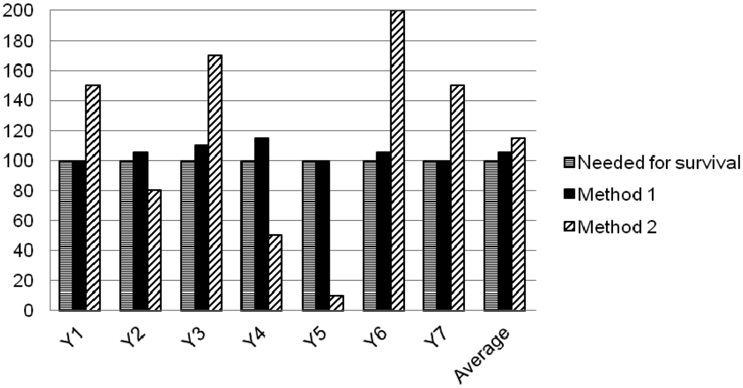
Similar preferences exist for human efforts [24]. A farming approach that secures constant average annual returns of 80% to 90% of a possible maximum will be preferred over one averaging 100% but having widely varying returns between 0% and 250%. This is because any shortfalls are a significant threat to food security and survival. In the below example (Figure 3), people requiring food to survive would prefer the food producing output Method 1 over the higher yielding but more volatile output Method 2 due to the possibility of shortfall (i.e., periods 2, 4 and 5 fall below the minimum survival requirements, assuming no storage).
1.1. Variability Risk in Finance
Over time, risk and its measurement have become core parts of both economic and financial theory. The behavioral or physical aspect that is optimized for risk varies widely by species (and among academic disciplines) and includes territory, time, caloric value, energy, mating opportunities, reputation effects, fairness, certainty, emotion and mood effects, and property. In economics, the optimized currency is typically described as “utility” (e.g., [23,24]). Bernoulli [25] noted that “expected utility” (expected return modified by risk preferences) differed from “expected value” (the strict payout multiplied by its probability). Von-Neuman and Morgenstern [26] further advanced the concept that rational individuals are risk averse and act as though they are maximizing expected utility. More recently, Prospect Theory advanced economists understanding of how people make choices involving risk by making the theory more psychologically realistic [18]. In essence, they posit that agents facing gains become more risk averse and those facing losses become more risk prone, consistent with the risk-sensitive foraging literature [27]. Finance has developed practical applications of these economic theories. In our financial system, investors can be thought of as optimal foragers; those with consistently high returns have more “energy” with which to buy goods and services as well as confer this advantage to their offspring. Interestingly, functional magnetic resonance scans of stock traders brains show the activation of the same prefrontal regions after successful trades as when primates find food likes nuts and berries [28,29]. Like any ecosystem, finance is about achieving high rewards with as little risk (and variability) as possible, and has developed multiple methods for risk assessment. Over the past several decades, researchers in academia and private industry tested and refined measurements of how investors respond to various financial problems and scenarios (see, for example, [30]).
In financial markets, risk is commonly measured by volatility, a statistical measure of the dispersion of returns for a given security or market index. Volatility is measured either by using the standard deviation or variance between returns from that same security or a market index. Essentially, the higher the volatility, relative to itself or to a benchmark, the riskier an investment becomes [31,32]. Modern portfolio theory has formalized investor's preferences for lower volatility (given returns of equal expected value) with a measure termed “risk adjusted return”, or the return per unit of standard deviation. In evaluating investment alternatives risk aversion lies at the core of risk-return models, such as mean-variance portfolio theory. Markowitz formalized the observation that investors are risk averse, and given two assets offering the same expected return, investors will prefer the less risky one [33]. Thus, an investor will take on increased risk only if compensated by higher expected returns. Although there are many ways to measure risk adjusted performance, one popular portfolio metric called “Sharpe Ratio” takes this concept one step further by measuring the amount of outsized return relative to a “risk free rate” for each unit of risk [34].
The Sharpe Ratio (real or ex ante) is thus the return of a given strategy minus the risk free rate of return (usually U.S. treasury bills) divided by the standard deviation of the return. Specifically:
Let's consider an example with four potential investments (A, B, C and, D). The assumed risk free rate is 3% (Table 2). The portfolio objective is an annual return of 5%, similar to the many pensions and endowments that have minimum return thresholds to pay out to their beneficiaries. As can be seen in Table 3, two dimensional (mean and volatility) return measures give a much more complete picture of investment success, though other nuances, such as maximum drawdown and relationship to a minimum accepted return are also important.
The advantage of risk metrics like the Sharpe Ratio is that one statistic generated from return histories (or expectations) gives the investor a meaningful way to compare investments with different means and variances. Given the above options an investor would likely choose option A as its risk adjusted expected return as far superior to the other 3 assets. Asset B, while having an overall higher return, has much more volatility, especially when compared to the minimum portfolio return of 5%. This higher volatility suggests a greater chance that future returns could fall short of the minimum required return. The return streams from assets C and D are considerably more volatile, including periods of losses. Their low risk adjusted returns drawdowns suggest they do not provide much return adjusted for risk. When an investor has a number of low risk investments that meet his minimum return target, those metrics identified above drive the decisions, e.g., he will select the investments with the highest Sharpe Ratio or similar statistic. Only in situations where the investor, in order to meet a minimum return target, has no choice but to accept investments with high risk (and thus relatively low Sharpe ratio), will he employ additional selection criteria. For example, he will try to create a portfolio mix of those lower quality investments that are least correlated in their fluctuations to eliminate part of the risk in the portfolio.
1.2. Applying Financial Risk Concepts to Net Energy Analysis
In energy systems, for example in electricity production, a similar need to reflect risk adjusted returns exists. For example, an index of electricity availability can be developed by multiplying the percent of a country's population with access to electricity by the percentage of hours in a year that there is uninterrupted electrical service. Figure 4 plots such an “availability index” compared against GDP/capita (purchasing power parity adjusted) for 99 countries. It shows that stable electricity is key to producing economic activity significantly above 10,000 US$/capita. The fact that no country with electricity availability below 98% exceeds a per capita GDP of US$ 20,000 suggests that electricity seems to be the prerequisite for high output, and not the inverse. The value of steadily available electricity at all times far exceeds the value of situations that experience regular blackouts, irrespective of the total amount of energy available. As we will show later, the electricity grid is a particularly fragile system, which is susceptible to deviations as small as 0.5% between demand and supply at any given point in time. Recently, fluctuations in the German electrical grid—where voltage weakened for only milliseconds—led to damage to at least one industrial production line, and the idling of that plant for several hours. Companies with sensitive production systems are investing in batteries and generators to prevent similar losses [35].
In general, energy supply technologies offer very different value to societies depending on how controllable they are. However, the importance of variability depends on the type of energy demand system. Storage-based energy sources such as oil, natural gas, or coal, (and to some extent hydropower), which are not subject to meaningful degradation, allow suppliers to maintain flows according to demand, with no or short ramp times required. They thus provide greater value and lower risk on the supply side. For example, oil exporting countries, in theory, can reduce oil production during periods of low demand and low prices. This approach maximizes the value extraction on the supply side, as the stores can be accessed primarily in a discretionary way.
In stock-based electricity production systems, conversion technologies (e.g., nuclear, coal, oil and gas generators) produce steady output flows. In these situations, inflexibility of supply can be managed. However, flow-based energy sources such as run-of-river hydropower, solar power, and wind energy, do not allow for supply-side control without additional investments and storage losses. To a certain extent, the same is true for energy conversion technologies that produce flows from stocks, but require long lead times to switch on or off once they are operational. For example, nuclear power plants and some coal based power plants incur significant efficiency reductions when changing their load. For these technologies, flows occur mostly independent of demand or prices.
Flow-based inputs with low and mostly only short-time horizon predictability like solar and wind power deliver output stochastically as a function of weather conditions. Once the infrastructure for these technologies has been installed (e.g., a photovoltaic panel, a wind turbine or a solar thermal concentrator) it can produce anything from 0% to 100% of nameplate capacity, relatively independent of demand. This does not necessarily translate to complete (short term) unpredictability, as weather forecasts are able to provide some limited planning guidance and PV panels produce the majority of their electricity during periods of high daytime demand; however, the overall delivery pattern is fully stochastic.
Deferral of supply of flow-based energy is possible only with storage technologies, which typically involve a significant conversion or entropy loss, and additional upfront investment. Conversely, gas, coal or oil based fuels can be stored at a high energy density for significant periods of non-use with only limited (for natural gas) or no storage losses (for oil and coal), and then used as needed. Electricity however, does not have that feature once it is produced—it is expensive to store, at a lower energy density, and always incurs losses. Electric power not used or stored at the time of its production is no longer usable even a few seconds later. In electricity systems, both over- and undersupply are equally detrimental, and if not managed, will lead to grid failures and blackouts. Currently, well over 90% of the U.S. energy supply is “stock based” [39]. A move to more “flow based” resources—run of river hydro, solar, wind, etc., will have large implications on how our energy systems are both structured, and used.
The largest human-made system that is based fully on short-term flow delivery is our electrical grid, infrastructure delivering electricity on demand using complex and intensively managed combinations of inputs. For these reasons we have chosen electricity supplying technologies to illustrate the important relationship of intermittence as it pertains to energy return for this paper. In electricity delivery systems, demand varies significantly throughout the hours of the day, days of the week and seasons of the year. Different generation technologies (driven by different energy sources), meet this intermittent demand in different ways. Below, electricity generation technologies are categorized according to their flow risks.
1.3. Stable Output Technologies
Run-of-river hydropower delivers steady outputs that are not typically easy to alter. This is largely also the case for nuclear and most coal power plants that convert stocks into flows and cannot be modulated easily. Their outputs vary little and are predictable for extended periods of time when considered in aggregate (i.e., while one power plant might fail, the aggregate supply of multiple plants using one technology typically delivers stable returns to a grid system). However, these technologies cannot transition their output either up or down in a timeframe short enough to meet typical demand fluctuations. These output changes are typically associated with energetic (and thus financial) losses. In situations where they supply electricity grids (as opposed to individual industrial facilities), these technologies are not flexible enough to follow all the peaks and lows demanded by society and therefore are of lower overall value. If they are only used against the portion of demand that is stable, their contribution becomes 100% valuable and highly predictable in aggregate.
We begin with a hypothetical example depicted in Figure 5, consistent with most demand curves for electricity for advanced economies of a day of operations of steady output sources in a network with a large proportion of stable outputs, for example—a country like France with a high share of nuclear power.
1.4. Flexible Technologies
Most stock-based technologies, like gas- or oil-fired power plants, or stored hydropower, can be modulated in a way that can directly follow demand patterns as they emerge. As such, they bear no demand shortfall risk in their application. However, in some cases, as these fuel types are the most valuable, they produce at relatively high costs (particularly true for oil-based generation, but similarly for natural gas).
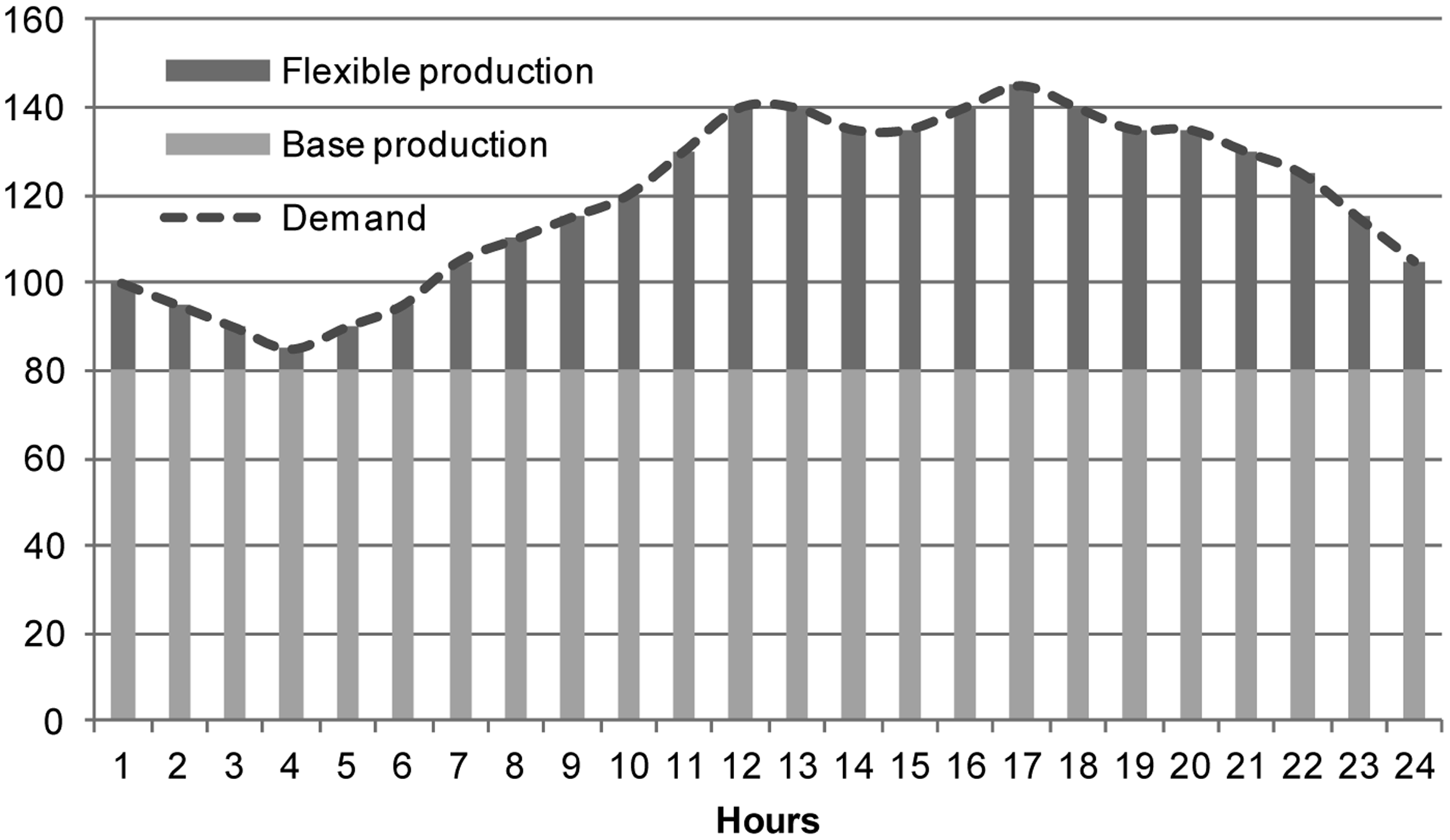
The example in Figure 6 illustrates an electricity grid composed of a stable base of steady output technologies (such as nuclear, coal or any combination thereof), supplemented with flexible generation capacity (such as stored hydropower or natural gas). Together, these technologies are able to match human demand perfectly.
1.5. Stochastic Technologies
Stochastic flow-based power generation techniques often show no or very limited correlation with demand, and deliver their energy outputs based on mostly independent variables like sunshine or wind. These may coincide partly with demand, as with solar power, which is produced during day-time high demand phases, however users have no control over this phenomenon and (depending on weather) output may appear or disappear almost completely across large areas within short periods of time. Furthermore, solar panels also produce when daytime demand is already met by other sources, for example during weekends and holidays.
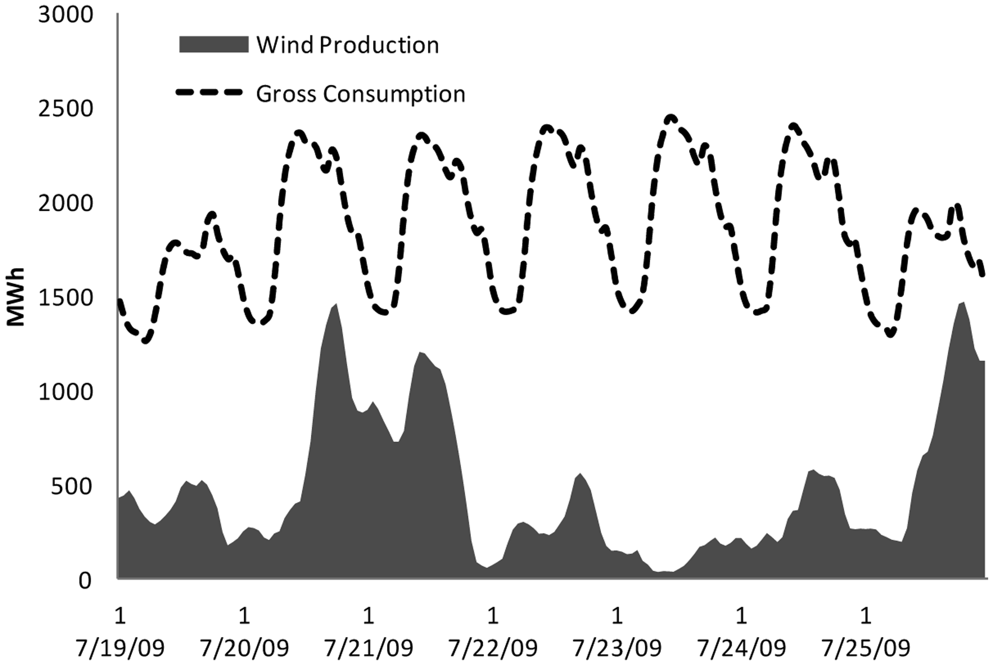
The example highlighted in Figure 7, shows a week of average wind power production and aggregate demand for Denmark from the summer of 2009. In this region, one of the best environments globally for wind power generation, wind supplies approximately 25% of total annual electricity demand. On an hourly basis, however, this coverage varies from 0% to 120% of total demand, across all hours of a typical year [40].
It is apparent from the above examples that two energy sources that may have the exact same net energy output provide different values to society, once their different delivery patterns are considered. Sources that are fully manageable or contribute steadily to ongoing demand are clearly preferable to sources supplying their outputs mostly uncorrelated to demand, when all other parameters are equal. Though this is relatively well understood among energy analysts, it has heretofore not been incorporated into energy quality calculations in biophysical economics.
2. Applications of a Risk Adjusted Energy Analysis
As discussed above, volatility in energy production causes problems, especially if the excess energy is not storable or requires costly investments to capture. To allow for a proper comparison of electricity generating technologies, negative impacts to the overall energy system (e.g., the electricity grid) need to be factored into the net energy calculations.
For inputs derived from stocks, the aggregate delivery risk of multiple plants is very low, as long as no major supply chain disruptions affect fuel availability. This paper explicitly does not deal with these large supply-side risks, although they can be considerable, such as dependence on foreign oil from volatile regions of the world. Instead we focus on a framework for measuring the short-term risks that result from mismatches between supply and demand.
Stable flows will provide less value to societies relative to sources with the ability to follow demand patterns as long as they cannot easily be adjusted to demand. The relevant volatility risk for all sources thus is not the physical variability of the supply itself, but the standard deviation of supply relative to consumption. This applies only to flow-based supply systems. Stock-based supply systems, where the final energy carrier is stored without conversion or loss, are much more tolerant to supply fluctuations (i.e., supply deviation relative to demand), as long as no system-wide undersupply threatens overall stability.
In order to simplify the analysis we assume a closed system, not factoring in transfers to and from other geographical areas. The relevant time interval for an analysis of risk adjusted net energy also largely depends on whether the final energy demand system is based on flows or stocks If the energy is used to feed a flow (such as an electricity grid), the variability at the shortest possible time interval should be measured. The interval of production (annually) is more appropriate for resources that are able to be stored (e.g., biofuels produced from various crops). Said differently, if energy quality decays almost immediately after its production, a proper analysis would have to use the smallest possible time interval to assess its utility to its flow based human use.
In order to arrive at a meaningful valuation of energy input risk, we test two methodologies to estimate the impact on variability on EROI. Given limited data availability, we focus on three energy inputs into electricity grids: nuclear power, wind power, and natural gas (which is fully flexible, assuming sufficient generation capacity is available). The aim of this paper is not to establish new EROI numbers, but instead to introduce and conceptualize the approach of variance adjustment in the review of energy in general. To accomplish this, we use both electricity demand and wind power data from West Denmark, because a complete data set is available, and Denmark is considered a very favorable location for large scale wind electricity production. For wind, we combine the two independent regions of the Danish system (West and East), as each integrates with different grid systems. We analyze real production data from Spain as well [41]. This country has lower average wind outputs (e.g., a lower capacity factor) when compared to Denmark, but better temporal output distribution due to its exposure to multiple, relatively independent weather systems.
In an attempt to quantify energy variability, we now introduce and compare two methodologies that can be applied to most available energy gathering or conversion technologies. The first method compares supply and demand, and penalizes an energy supply technology in proportion to the gaps between the two. The second methodology quantifies the energy cost of mitigation, e.g., the additional energy required either by adding flexible generation capacity (Method 2) to handle the supply/demand mismatches.
2.1. Method 1: Supply-Demand Comparison
In the first methodology, we introduce a handicap for each unit of energy that deviates from total demand, based on a long enough time period (a year) where energy supply is scaled to meet energy demand. In this approach an energy system is modeled as if one technology alone would supply a fixed demand system, and is similar to measuring whether the technology can be expected to supply a fixed percentage of total demand. Here we assume that all deviations from demand incur a cost to the overall system to compensate for variability. This cost determines the handicap for a particular technology.
We compare three production scenarios, an inflexible system producing all power from nuclear power plants, a fully flexible grid only using gas powered turbines, and wind electricity production for West Denmark, combined Denmark (East and West), and Spain all scaled up to cover 100% of electricity demand over a year. To scale up wind electricity generation, we multiply hourly wind production by a constant, which results in annual electricity demand equal to total wind production. This preserves the electricity output variation over the year, at the hourly scale. These hypothetical supply patterns are compared with electricity consumption. All calculations are on an hourly basis. Over one year, the gaps between supply and demand for each technology are cumulated, and this sum relative to the total is considered a “handicap” to the nominal energy gain of a particular technology.
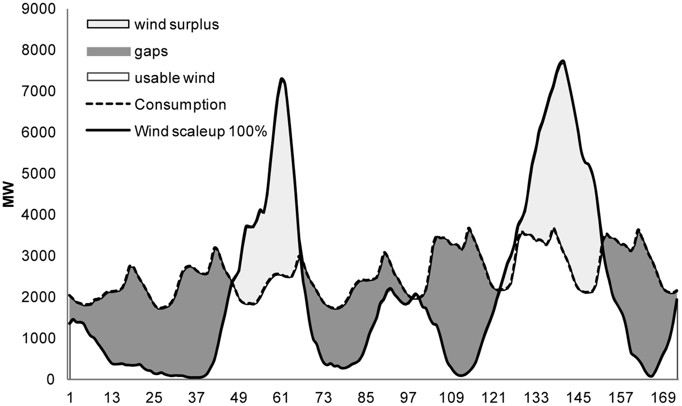
Figure 8 illustrates this approach for wind power generation. The dashed black line represents electricity demand, in hourly intervals, throughout a period of approximately one week. A flow-based source (in this case wind) produces energy in a pattern represented by the solid line, which on average produces energy matching demand for the entire year. However, this energy harvesting technology shows significant deviation from what is a regular demand pattern. Relative to the demand line, there are periods where it significantly over- and under-produces. The risk-adjusted EROI thus has to account for lost energy due to waste (the light gray areas) and periods of shortfall requiring an energy subsidy from another source (the dark gray areas). To obtain an accurate net energy statistic, the sum of all light gray areas during the technology's life cycle need to be deducted from nominal EROI. Similarly, the sum of all the dark gray areas, if another energy source was required to come online to meet human demand, would also be deducted. All these periods of variability relative to demand are then cumulated to obtain a handicap to the nominal EROI metric.
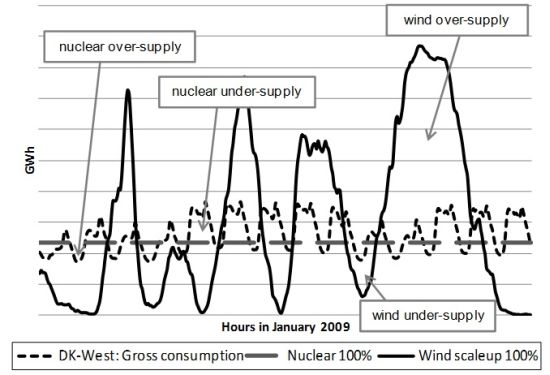
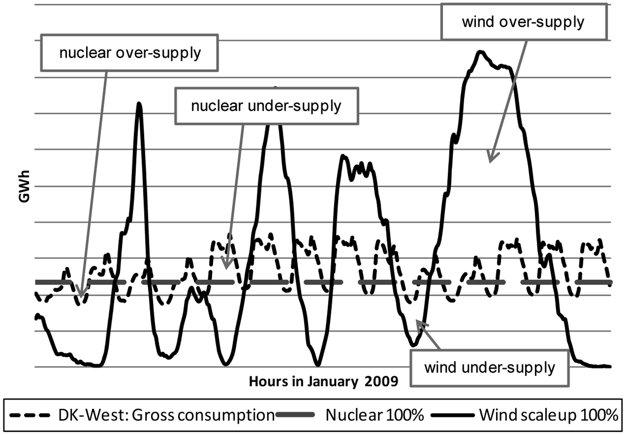
Figure 9 depicts Denmark West electricity consumption during the first 14 days (336 h) in January 2009. Overlaid are hypothetical supply curves for 100% coverage with nuclear power and 100% coverage with scaled-up wind power. Both the negative and positive supply gaps create problems for the grid system and thus need to be accounted for, which is quantified in Table 4 below using data for the entire year 2009. For comparison, we also include 2007 and 2008 data for Denmark West, which shows only small deviations from 2009.
Under Method 1, the EROI for nuclear power would be discounted by 19.8%, whereas nominal wind EROI gets discounted by a factor of 49.4% (best case) to 70.5% (worst case). In other words, if wind has an undiscounted EROI of 19.2 [15], the effective EROI after adjusting for intermittency risk would be reduced by an average of 60%, down to 7.7. Similarly, if nuclear power is rated with an EROI of 5–15 [8], a handicap of 20% would reduce its EROI to 4–12, while a flexible source like natural gas (only the generation component) would not face further handicaps based on variability.
This methodology can be represented using Equation (2), where d is demand and s is supply:
For energy systems which do not require a handicap for oversupply (e.g., producing a stock that can be stored easily and without losses), only the areas below the curve would need to be discounted. It may even be argued that discounting is unnecessary, as long as fluctuations do not exceed a certain level.
2.2. Method 2: Gap-Matching View
An alternative method for integrating variability risk with energy gain is to use existing technologies capable of filling the gaps left by the technology studied. While surpluses are still lost and need to be part of the technology handicap, supply shortfalls can be filled with a compensating technology. Such a buffer technology must be capable of filling the largest possible gap, even if this occurs only once. If this were not the case, the system (in this case the electricity grid) would fail at that moment [42].
In this analysis, the handicap needs to be applied from the energy cost of providing the technology alternative, less its fuel cost. So if, in the example below, gas turbines need to be kept permanently in non-spinning reserve service, i.e., in reserve and ready to be operated in order to match the supply gaps from nuclear power or wind, the energy (or money) needed to provide this additional infrastructure must be accounted for. Today's market mechanisms are not built around low-frequency (a few times a year) high demand events (e.g., no wind for a long time), but rather for high-frequency (a few times per week) and low-demand (e.g., a power plant failure or unexpected low output from one or more sources. For this reason in this analysis we look at the full cost of requiring this extra capacity present and idling.
For the same technologies analyzed in Method 1, we assume compensation of supply gaps with natural gas power for Method 2. As energy data for gas power are sparse, we use monetary production costs to approximate total handicaps from matching supply gaps. The cost of providing the alternative technology is equal to the total cost of keeping the capacity available to match the largest gap in supply from the original source (in this case nuclear or wind power). Fuel costs are not included, as gas delivers additional energy to the grid.
For the gap-matching analysis, these calculations are based on total ex-power plant production cost (not including any grid connection). There are multiple, sometimes conflicting, sources of estimates for the levelized cost per kWh for natural gas, nuclear and wind power [43–45]. For this simulation, we assume a cost of 8 cents per kWh for natural gas electricity generation, and 8 cents for nuclear electricity generation. For natural gas, we calculate investment and operations cost based on normal operations estimates available from [43,44] and assume a 2.2 cent per kWh fixed operations and maintenance cost for normal use (35% utilization). In order to arrive at an appropriate cost, both investment and operations costs need to be attributed to each unit of energy (kWh) produced from the source technology (e.g., wind or nuclear in this case). The underutilization of gas power plants when compared to normal operating modes needs to be factored in, resulting in a higher price, as is indicated in Table 5.
Table 6 summarizes the resulting calculations. It is evident that the handicaps evaluated using Method 2 are very similar to the ones obtained using a strictly mathematical formulation as in Method 1. Wind would—based on Denmark West data, receive a handicap of 71.2% (vs. 70.5% in Method 1), and nuclear a handicap of 23.6% (vs. 19.8 from Method 1).
The purpose of approximating a variability handicap for EROI statistics is to discover the true energy gain available to society using different individual technologies. Ultimately, when concerned with sustainability, we should be able to construct an energy system without any fossil fuel stocks, and rely completely on flows. To measure how much such a system costs in energy terms, would require (first) a standalone analysis of the relevant renewable technologies. An interesting, but completely different objective would be to create a “portfolio EROI” where X% of Technology A is combined with Y% of Technology B to come up with a blended Portfolio C. While it is true that incorporating nuclear or wind or solar energy into a grid will cause less fossil fuel to be used per month/year, it is the energy cost we are concerned with. Therefore the calculation of a standalone energy statistic, as attempted in this paper, is a necessary starting point.
3. Discussion
When accounting for risks in delivering energy technologies, Methods 1 and 2 delivered highly comparable results despite the relative uncertainty regarding the cost model used in Method 2. Thus, it seems appropriate to introduce handicaps according the deviations between supply and demand in flow-based output systems such as electricity grids. As indicated in Table 7, this handicap range, depending on the method and the location, is significant relative to nominal EROI for wind and nuclear.
As we have attempted to demonstrate here, developing a metric for risk-adjusting energy flows seems not only important but feasible. It remains an open question how to develop a similar methodology for application to stock based energy systems. Due to fungibility and transportability on global markets, the fluctuations and risk of individual coal, oil and natural gas wells, fields or mines, represents a different sort of risk, one that is less relevant to the aggregate energy gain of a specific technology, since all these energy types are storable once procured. Also, the availability of complete energy data is limited, posing another difficulty in establishing a similar metric. Ultimately however, the importance of variability matters most for the key flow-based energy system for societies: the electricity grid. Applied to this, the initial approach appears to return valid results.
Table 8 applies the most common financial risk metric, the Sharpe Ratio, to EROI analysis. The “Sharpe EROI” is related to but not actually equivalent to the monetary “Sharpe” ratio which is based on annual returns while the EROI Sharpe ratio is based upon total return over the lifetime of an energy technology. The numerators both refer to the “mean” return but the denominator in our case is the standard deviation of continuous, as opposed to annual returns. Several energy sources were measured first obtaining EROI from the median reported numbers in recent literature [3]. Then, the standard deviation of a source's energy delivery against human demand was computed on an hourly basis throughout one year using the datasets above. Given its ability to fill on demand electricity use, natural gas is viewed as “risk free” energy asset from an intermittence perspective. Though able to switch on and off similar to gas, coal has—particularly for non-anthracite qualities—a lead time between 6 and 12 h and therefore can only follow larger patterns (weekdays/weekends). The calculations assumed one daily load change. For solar, where no aggregate data is available due to the distributed nature of photovoltaic installations without central metering, a stochastic pattern was assumed comparable to wind, but with a higher correlation to human demand patterns due to the fact that sunshine is available throughout the day.
A “Net Energy Sharpe Ratio” was then computed by taking the nominal EROI numbers, subtracting out the risk free rate, and dividing by standard deviation (Equation (3), Table 8). Conceptually, this should rank fuels based on their intermittence/quality adjusted values relative to a human demand system. After natural gas, based on its high initial EROI, coal offers the highest “Sharpe EROI”, followed by nuclear. Wind and solar power experience significant handicaps due to high deviations compared to human demand patterns. Thus, from, the perspective of “excess return versus a benchmark”, coal and particularly natural gas exhibit high return for each unit of risk, while other sources come out significantly weaker:
As within financial theory, a risk adjusted EROI will help sort energy inputs into a “portfolio” of technologies to contribute towards the final supply output. Societies can then select the technologies/sources with the highest risk-adjusted energy returns first, and combine them into a portfolio. If the technologies delivering the best results are no longer available or feasible (for example due to external restrictions), alternatives will have to be evaluated based on a careful analysis of their correlations to one another. Low or even negatively correlated output methods might—in a portfolio of technologies—partly offset their risks.
In this paper we focused on variability risks. Other risks not covered here are also relevant when making decisions about future energy sources. One such risk, measuring the timing of flows in energy gathering and conversion risk, also bears further study (see [47], for an overview). In a companion paper, we adjusted the timing of energy inputs and outputs over the lifecycle of selected energy technologies, and handicapped each flow by a discount rate, thus more heavily weighting both inputs and outputs that occur closer to now (time zero). Integrating both time and variability risk gives a fuller sense of how a particular technology/source fits with human demand profile for energy services. Table 9 indicates, at various discount rates, a preliminary look at the combined handicap (Time + Variability) for Wind and Solar Photovoltaic. At a 20% discount rate, the adjusted EROI from a base case for solar of 8:1 drops to a sub-unity EROI of 0.9:1.
Ultimately, in a comprehensive framework on energy and risk, time and variability are key risks, but environmental externalities, natural disasters and weather related shortfalls, geopolitical risks, and other general systemic risks that are inherent in energy delivery systems would need to be integrated as well. The higher the impact of disruptions (in flow-based systems), the larger the problems with stochastic or unreliable inputs becomes, as it not only creates a direct gap, but also threatens systems stability.
The intermittency of wind power production (and other stochastic sources) thus creates systemic and structural risks. In this context, “systemic risk” defines risk that is tied to the hour-to-hour operation of the energy grid. Renewable electricity generation technologies which directly deliver into the grid based on stochastic input flows (like sun or wind) are thus heavily challenging the entire system and need to be handicapped accordingly when their energy returns are assessed. Ultimately, their imbalances cause problems or additional cost in the system, even if this cost is disguised.
4. Conclusions
Risk versus reward is a central theme in nature, particularly with respect to energy capture. This paper was a first attempt at conceptualizing the impact of variability to common biophysical statistics. When introducing supply risk into a review of energy technologies, both reliability and manageability become very important, as they define the benefit of a technology to society. Though the physical volatility and intermittency of energy are themselves important variables, it is their relationship to societal demand that ultimately defines how relevant risk becomes. Finance suggests that the covariance of a project's return with the return to the economy as a whole is what matters, not the covariance with itself. Similarly, a nominally high EROI statistic may not be of high value as a policy choice if its risk and intermittency are not considered. In summary, the costs associated with increased variance from renewable electricity generation technologies may be a larger drawback than nominal biophysical measures indicate. Further research incorporating risk as a factor into energy quality is warranted.
Conflicts of Interest
The authors declare no conflict of interest.
References
- Lotka, A.J. Contribution to the energetics of evolution. Proc. Natl. Acad. Sci. USA 1922, 8, 147–151. [Google Scholar]
- Odum, H.T. Environment, Power, and Society; Wiley-Interscience: New York, NY, USA, 1970. [Google Scholar]
- Hall, C.A.S.; Balogh, S.B.; Murphy, D.J.R. What is the minimum EROI that a sustainable society must have? Energies 2009, 2, 25–47. [Google Scholar]
- Lambert, J.G.; Hall, C.A.S.; Balogh, S.; Gupta, A.; Arnold, M. Energy, EROI and quality of life. Energy Policy 2014, 64, 153–167. [Google Scholar]
- Hannon, B. Energy discounting. Technol. Forecast. Soc. Chang. 1982, 21, 281–300. [Google Scholar]
- Cleveland, C.J. Energy quality and energy surplus in the extraction of fossil fuels in the U.S. Ecol. Econ. 1992, 6, 139–162. [Google Scholar]
- Tainter, J.A. The Collapse of Complex Societies; Cambridge University Press: Cambridge, UK, 1988. [Google Scholar]
- Morgan, T. Brave New World? Issues in the New Decade; Tullett Prebon Group, Ltd.: London, UK, 2010. Available online: http://www.tullettprebon.com/Documents/strategyinsights/tp1109d_TPSI_report_002_LR.pdf (accessed on 25 September 2012.
- Lambert, J.G.; Hall, C.A.S.; Balogh, S.; Poisson, A.; Gupta, A. EROI of Global Energy Resources—Preliminary Status and Trends; Report to UK Department for International Development (DFID): London, UK, 2012. [Google Scholar]
- Gilliland, M.W. Energy analysis and public policy. Science 1975, 189, 1051–1056. [Google Scholar]
- Gagnon, N.; Hall, C.A.S.; Brinker, L. A preliminary investigation of energy return on energy investment for global oil and gas production. Energies 2009, 2, 490–503. [Google Scholar]
- Cleveland, C.J. Net energy from the extraction of oil and gas in the United States. Energy 2005, 30, 769–782. [Google Scholar]
- Lenzen, M.; Munksgaard, J. Energy and CO2 life-cycle analyses of wind turbines—Review and applications. Renew. Energy 2002, 26, 339–362. [Google Scholar]
- Hall, C.A.S. The Energy Return of (Industrial) Solar—Passive Solar, PV, Wind and Hydro (#5 of 6). Available online: http://www.theoildrum.com/node/3910 (accessed on 10 May 2010).
- Kubiszewski, I.; Cleveland, C.J.; Endres, P.K. Meta-analysis of net energy return for wind power systems. Renew. Energy 2010, 35, 218–225. [Google Scholar]
- Battisti, R.; Corrado, A. Evaluation of technical improvements of photovoltaic systems through life cycle assessment methodology. Energy 2005, 30, 952–967. [Google Scholar]
- Farrell, A.E.; Plevin, R.J.; Turner, B.T.; Jones, A.D.; O'Hare, M.; Kammen, D.M. Ethanol can contribute to energy and environmental goals. Science 2006, 311, 506–508. [Google Scholar]
- Kahneman, D.; Tversky, A. Prospect theory: An analysis of decision under risk. Econometrica 1979, 47, 263–291. [Google Scholar]
- Weber, E.U.; Shafir, S.; Blais, A. Predicting risk sensitivity in humans and lower animals: Risk as variance or coefficient of variation. Psychol. Rev. 2004, 111, 430–445. [Google Scholar]
- International Organization for Standardization (ISO). Risk Management—Vocabulary; ISO 31000:2009/ISO Guide 73:2002; ISO: Geneva, Switzerland, 2009. [Google Scholar]
- Caraco, T.; Martindale, S.; Whittam, T.S. An empirical demonstration of risk-sensitive foraging preferences. Anim. Behav. 1980, 28, 820–830. [Google Scholar]
- Bateson, M. Recent advances in our understanding of risk-sensitive foraging preferences. Proc. Nutr. Soc. 2002, 61, 509–516. [Google Scholar]
- Kacelnik, A.; Bateson, M. Risky theories—The effects of variance on foraging decisions. Am. Zool. 1996, 36, 402–434. [Google Scholar]
- Chabris, C.; Laibson, D.; Schuldt, J. Intertemporal Choice. In The New Palgrave Dictionary of Economics, 2nd ed.; Palgrave Macmillan: London, UK, 2008. [Google Scholar]
- MacArthur, R.H.; Pianka, E.R. On the use of a patchy environment. Am. Nat. 1966, 100, 603–610. [Google Scholar]
- Bernoulli, D. Exposition of a new theory on the measurement of risk. Econometrica 1954, 22, 23–36. [Google Scholar]
- Von Neumann, J.; Morgenstern, O. Theory of Games and Economic Behavior, 3rd ed.; Princeton University Press: Princeton, NJ, USA, 1953. [Google Scholar]
- Kacelnik, A. The Evolution of Patience. In Time and Decision: Economic and Psychological Perspectives on Intertemporal Choice; Loewenstein, G., Read, D., Baumeister, R., Eds.; Russell Sage Foundation: New York, NY, USA, 2003; pp. 115–138. [Google Scholar]
- Wise, R.A. Role of brain dopamine in food reward and reinforcement. Philos. Trans. R. Soc. B Biol. Sci. 2006, 361, 1149–1158. [Google Scholar]
- Lehrer, J. How We Decide; Houghton Mifflin Harcourt: Boston, MA, USA, 2009. [Google Scholar]
- Lo, A.W. Risk management for hedge funds: Introduction and overview. Financ. Anal. J. 2001, 57, 16–33. [Google Scholar]
- Sharpe, W.F. Mutual fund performance. J. Bus. 1966, 39, 119–138. [Google Scholar]
- Biglova, A.; Ortobelli, S.; Rachev, S.T.; Stoyanov, S. Different approaches to risk estimation in portfolio theory. J. Portf. Manag. 2004, 31, 103–112. [Google Scholar]
- Markowitz, H. Portfolio Selection; Efficient Diversification of Investments; Yale University Press: New Haven, CT, USA, 1970. [Google Scholar]
- Sharpe, W.F. The Sharpe ratio. J. Portf. Manag. 1994, 21, 49–58. [Google Scholar]
- Schroder, C. Grid Instability has Industry Scrambling for Solutions. Der Spiegel, 13 August 2012. Available online: http://www.spiegel.de/international/germany/instability-in-power-grid-comes-at-high-cost-for-german-industry-a-850419.html (accessed on 12 September 2012). [Google Scholar]
- World Development Indicators Database. Washington, DC, USA: World Bank, 2011. Available online: http://siteresources.worldbank.org/DATASTATISTICS/Resources/GDP_PPP.pdf (accessed on 17 March 2010).
- Earth Trends. Washington, DC, USA: World Resources Institute. Available online: http://earthtrends.wri.org/searchable_db/index.php?theme=6&variable_ID=1379&action=select_countries (accessed on 19 February 2010).
- Business Environment and Enterprise Performance Survey (BEEPS). European Bank for Reconstruction and Development: London, UK. Available online: http://www.ebrd.com/pages/research/analysis/surveys/beeps.shtml (accessed on 15 March 2010).
- Energy Information Administration (EIA). Annual Energy Review. The Administration: Washington, DC, USA. Available online: http://www.eia.doe.gov/aer/ (accessed on 21 November 2010).
- Danish Electricity Market Data. Energinet: Fredericia, Denmark. Available online: http://www.energinet.dk/EN/El/Engrosmarked/Udtraek-af-markedsdata/Sider/default.aspx (accessed on 24 November 2010).
- Energy Demand in Real Time. Red Electrica De Espana: Madrid, Spain. Available online: https://demanda.ree.es/demandaGeneracionAreasEng.html (accessed on 16 August 2010).
- Operations Handbook Policy 1—Load Frequency Control European Network of Transmission System Operators for Electricity (ENTSO-E). Brussels, Belgium. Available online: http://www.entsoe.eu/fileadmin/user_upload/_library/publications/ce/oh/Policy1_final.pdf (accessed on 19 May 2010).
- International Energy Agency (IEA); Nuclear Energy Agency (NEA). Projected Costs of Generating Electricity—2010 Edition; IEA: Paris, France, 2010.
- Energy Information Administration (EIA). 2016 levelized Cost of New Generation Resources from the Annual Energy Outlook 2010. Available online: http://www.eia.doe.gov/oiaf/aeo/pdf/2016levelized_costs_aeo2010.pdf (accessed on 21 August 2010).
- Heptonstall, P. A Review of Electricity Unit Cost Estimates; Working Paper for UK Energy Research Centre: London, UK, 2007. [Google Scholar]
- Hagens, N.J.; Kunz, H. Applying Time to Energy Analysis. Available online: http://www.theoildrum.com/node/7147 (accessed on 23 December 2013).


| Energy technology | EROI | Reference |
|---|---|---|
| Global oil production | 35 | [11] |
| Coal (mine mouth) | 80 | [12] |
| Nuclear | 5–15 | [13] |
| Hydropower | >100 | [14] |
| Wind turbines | 18 | [15] |
| Solar photovoltaic | 6–8 | [16] |
| Corn based ethanol | 0.8–1.6 | [17] |
| Year 1 | Year 2 | Year 3 | Year 4 | Year 5 | Year 6 | Year 7 | Year 8 | Year 9 | Year 10 | Mean | |
|---|---|---|---|---|---|---|---|---|---|---|---|
| Minimum | 5% | 5% | 5% | 5% | 5% | 5% | 5% | 5% | 5% | 5% | 5.0% |
| Risk free rate | 3% | 3% | 3% | 3% | 3% | 3% | 3% | 3% | 3% | 3% | 3.0% |
| Investment A | 8% | 10% | 8% | 10% | 8% | 10% | 8% | 10% | 8% | 10% | 9.0% |
| Investment B | 15% | 5% | 15% | 5% | 15% | 5% | 15% | 5% | 15% | 5% | 9.9% |
| Investment C | −9% | 15% | 39% | 20% | −4% | −14% | 28% | −12% | 26% | 15% | 8.9% |
| Investment D | 3% | 2% | 8% | −4% | 10% | 8% | −6% | 4% | −8% | 14% | 3.1% |
| Asset | Mean return | Standard deviation | Risk adj. return | Sharpe ratio |
|---|---|---|---|---|
| Risk Free | 3.0% | 0% | n/a | n/a |
| A | 9.0% | 1% | 9.0 | 6.0 |
| B | 9.9% | 5% | 2.0 | 1.4 |
| C | 8.9% | 17.9% | 0.50 | 0.3 |
| D | 3.0% | 6.9% | 0.43 | 0.0 |
| Total consumption | Undersupply | Oversupply | Total Gap | Handicap to EROI | |
|---|---|---|---|---|---|
| Gas power DK West (2009) | 20,550 GWh | 0 GWh | 0 GWh | 0 GWh | 0% |
| Hypothetical linear output source (Nuclear) in DK West (2009) | 20,550 GWh | 2,038 GWh | 2,038 GWh | 4,077 GWh | 19.8% |
| Wind DK West (2009) | 20,550 GWh | 7,243 GWh | 7,243 GWh | 14,486 GWh | 70.5% |
| Wind DK West (2008) | 21,622 GWh | 7,942 GWh | 7,942 GWh | 15,884 GWh | 73.5% |
| Wind DK West (2007) | 21,596 GWh | 7,946 GWh | 7,946 GWh | 15,892 GWh | 73.6% |
| Wind DK combined (2009) | 34,591 GWh | 11,875 GWh | 11,875 GWh | 23,749 GWh | 68.7% |
| Wind Spain (2009) | 251,630 GWh | 61,102 GWh | 61,102 GWh | 124,204 GWh | 49.4% |
Note that over- and undersupply are identical because sources are scaled up to 100%.
| Natural gas compensating wind in West Denmark for 2009 [46] | Base cost per kWh of wind: | US$ 0.08/kWh |
| Investment cost gas turbine: | US$ 1,270/kWe | |
| Fixed operation and maintenance: a | US$ 0.022 $/kWe | |
| Life expectancy of plant: | 12.5 years | |
| Capacity requirement (largest gap): | 3.5 GWe | |
| Total investment into capacity b: | US$ 4,445 million | |
| Total annual consumption (2009): | 20,550 GWh | |
| Gaps to cover: | 7,243 GWh | |
| Utilization: c | 23.6% | |
| Operations cost per kWh: d | US$ 0.033 | |
| Investment cost per annum: | US$ 355.6 million | |
| Operations cost per annum: | US$ 256.1 million | |
| Total cost per annum e: | US$ 591.7 million | |
| Total cost per kWh of wind output f: | US$ 0.029 | |
| Handicap (% of 8¢ base cost/kWh): | 36.0% (2.9 ¢/8 ¢) | |
| Natural gas compensating wind in Spain (2009) | Capacity requirement (largest gap): | 38.1 GWe |
| Total investment into capacity b: | US$ 4,445 million | |
| Total annual consumption (2009): | 251,630 GWh | |
| Gaps to cover: | 62,102 GWh | |
| Utilization: c | 18.6% | |
| Operations cost per kWh: d | US$ 0.041 | |
| Investment cost per annum: | US$ 6,876 million | |
| Operations cost per annum: | US$ 2,574 million | |
| Total cost per annum e: | US$ 6,460.7 million | |
| Total cost per kWh of wind output f: | US$ 0.026 | |
| Handicap (% of 8¢ base cost/kWh): | 32.0% | |
| Natural gas compensating nuclear power | Base cost per kWh of nuclear power: | US$ 0.08 |
| Capacity requirement (largest gap): | 1.33 GWe | |
| Total investment into capacity b: | US$ 1,689 million | |
| Total annual consumption (2009): | 20,550 GWh | |
| Gaps to cover: | 2,038 GWh | |
| Utilization: c | 17.5% | |
| Operations cost per kWh: d | US$ 0.044 | |
| Investment cost per annum: | US$ 135.1 million | |
| Operations cost per annum: | US$ 89.7 million | |
| Total cost per annum e: | US$ 224.8 million | |
| Total cost per kWh of nuclear output f: | US$ 0.011 | |
| Handicap (% of 8¢ base cost/kWh): | 13.7% | |
aat 35% utilization;bTotal investment into capacity: Largest Gap * 1000 (MWe-GWe) * investment cost gas turbine;cOperations cost per KWh: Operations cost (no fuels) * 1.5 (ballpark correction for underuse;cused to correct operations cost;dOperations cost per annum: Gaps to cover * Operations cost per kWh;eTotal cost per annum: Investment cost + operations cost p.a.;fTotal cost per kWh of wind output: Total cost p.a./annual wind production.
| Type of fuel and nameplate capacity | Total consumption | Oversupply | Oversupply handicap (Total cons./Oversupply) | Largest supply gap | Cost of supply gap in % of base technology cost | Total EROI Handicap (Oversupply + supply gap handicaps) |
|---|---|---|---|---|---|---|
| Nuclear (∼2.35 GWe) | 20,550 GWh | 2,038 GWh | 9.9% | 1.33 GW | 13.7% | 23.6% |
| Wind DK West (∼10 GWe) | 20,550 GWh | 7,243 GWh | 35.2% | 3.5 GW | 36.0% | 71.2% |
| Wind Spain (∼145 GWe) | 251,630 GWh | 62,102 GWh | 24.6% | 38.1 GW | 32.0% | 56.6% |
| Technology | EROI (undiscounted) | Method 1 | Method 2 |
|---|---|---|---|
| Wind | 19.2 | 5.7–9.7 (location-dependent) | 5.5–8.3 (location-dependent) |
| Nuclear | 5–15 | 4–12 | 3.8–11.5 |
| EROI of primary energy EROI | Electricity conversion C | Power plant P | EROI of electricity EROI(net) = EROI * (C−P) | Std dev. from demand | EROI(net)−rf | Return Standard Deviation σp | “Sharpe” EROI | |
|---|---|---|---|---|---|---|---|---|
| Gas | 15 | 45% | 5% | 6 | 0.0% | 0 | n/a | n/a |
| Coal | 60 | 35% | 5% | 18 | 20.9% | 12.0 | 3.8 | 3.2 |
| Nuclear | - | - | - | 10 | 23.0% | 4.0 | 2.3 | 1.7 |
| Wind | - | - | - | 19.2 | 86.8% | 13.2 | 16.7 | 0.8 |
| Solar | - | - | - | 8 | 75.0% | 2.0 | 6.0 | 0.3 |
| Disc. Rate ≥ | 5% | 5% | 10% | 10% | 15% | 15% | 20% | 20% | |
|---|---|---|---|---|---|---|---|---|---|
| Nominal EROI | Time | Time + Var | Time | Time + Var | Time | Time + Var | Time | Time + Var | |
| Wind | 19.2 | 12.4 | 7.4 | 8.6 | 5.2 | 6.4 | 3.8 | 5.0 | 3.0 |
| Solar PV | 8.0 | 5.1 | 2.5 | 3.3 | 1.7 | 2.3 | 1.2 | 1.7 | 0.9 |
© 2014 by the authors; licensee MDPI, Basel, Switzerland. This article is an open access article distributed under the terms and conditions of the Creative Commons Attribution license ( http://creativecommons.org/licenses/by/3.0/).
Share and Cite
Kunz, H.; Hagens, N.J.; Balogh, S.B. The Influence of Output Variability from Renewable Electricity Generation on Net Energy Calculations. Energies 2014, 7, 150-172. https://doi.org/10.3390/en7010150
Kunz H, Hagens NJ, Balogh SB. The Influence of Output Variability from Renewable Electricity Generation on Net Energy Calculations. Energies. 2014; 7(1):150-172. https://doi.org/10.3390/en7010150
Chicago/Turabian StyleKunz, Hannes, Nathan John Hagens, and Stephen B. Balogh. 2014. "The Influence of Output Variability from Renewable Electricity Generation on Net Energy Calculations" Energies 7, no. 1: 150-172. https://doi.org/10.3390/en7010150