Taxing Strategies for Carbon Emissions: A Bilevel Optimization Approach

Abstract

This paper presents a quantitative and computational method to determine the optimal tax rate among generating units. To strike a balance between the reduction of carbon emission and the profit of energy sectors, the proposed bilevel optimization model can be regarded as a Stackelberg game between the government agency and the generation companies. The upper-level, which represents the government agency, aims to limit total carbon emissions within a certain level by setting optimal tax rates among generators according to their emission performances. The lower-level, which represents decision behaviors of the grid operator, tries to minimize the total production cost under the tax rates set by the government. The bilevel optimization model is finally reformulated into a mixed integer linear program (MILP) which can be solved by off-the-shelf MILP solvers. Case studies on a 10-unit system as well as a provincial power grid in China demonstrate the validity of the proposed method and its capability in practical applications.

1. Introduction

Global climate change is mostly attributed to the excessive emission of greenhouse gases, especially carbon dioxide (CO₂). According to [1], the concentration of CO₂ in the Earth's atmosphere has grown by 35% since the Industrial Revolution. The emissions of CO₂ will still increase by 1.9% annually if no effective action is taken. The strong requirement for a cleaner environment and sustainable development brings new challenges to all emission intensive sectors.

In order to combat global warming issues, many countries have launched their future plans in emission reduction and devoted substantial efforts to achieve their goals through some market-based policies. Such policies regulate customers' behavior through market forces. Briefly speaking, the emission of CO₂ would be reduced if the price of emission intensive products increases and consequently the demands shift to other alternative environmentally-friendly goods. From an economic point of view, market-based policies effectively achieve the target of emission reduction at the lowest cost to society [2]. Among various market based policies, the cap-and-trade (C&T) program [3] and carbon tax scheme [4] are the most widely implemented regulations.

In the C&T program, a government agency specifies a limit or cap on the total amount of carbon emissions. Then the cap is allocated to entities under regulation in the form of carbon credits. Generation companies (GENCOs) whose carbon credits are more than their actual emissions are allowed to trade them [3]. In the trading market, the buyer is charged for polluting the environment, while the seller is rewarded for protecting the environment. In practice, the European Union Emissions Trading System, known as the first and largest emissions trading system in the world [5], has become the key tool for reducing greenhouse gas emissions in Europe. The workings of spot, forward, future and option markets are studied in [6], the economic analysis is carried out in [7] and examined among 12 European countries. In the United States, a national market for SO₂ trading and several regional markets for nitrogen oxides trading have been established since 1990. Other countries such as New Zealand and Japan have also set up their own CO₂ trading programs.

The carbon tax is a direct charge imposed on carbon emissions. GENCOs are obligated to pay fees proportional to the quantity of their emissions. In the early 1990s, Sweden became the first country attempting to manage the carbon emission with the carbon tax scheme. In the following 20 years, a number of countries have tried to implement carbon tax or energy tax schemes that aim at reducing carbon emissions [8–10] and obtained positive effects. In 2009, the Chinese Ministry of Finance, together with the National Development and Reform Commission, promulgated a research report on the feasibility of implementing carbon tax policy in china, and announced future plans in the coming decade.

There has been a hot debate between C&T and carbon tax scheme [11–14]. Some argued that the carbon tax is easy to carry out since it does not require trading platforms. Moreover, it provides a price signal that stimulates emitters to seek long-term solutions such as investing on renewable generation sources [12]. But others insists that C&T has some distinctive advantages over a carbon tax, such as international fairness, broad participation, and most important, direct regulation on the total quantity of emissions [11]. It's worth mentioning that a comprehensive bilevel optimization model was proposed in [14] to investigate and compare the C&T and carbon tax policies in terms of effectiveness and efficiency from a generation expansion planning perspective. Relative advantages and disadvantages of both policies with respect to different criteria were revealed.

Despite the debate about C&T and carbon tax policy, a couple of strategic approaches have been studied to reduce carbon emission from energy and manufacturing industry. An inexact mix-integer two-stage program model was proposed in [15] for long term decision making problems under uncertainty, such as capacity expansion, facility improvement as well as coal inventory planning. A low-carbon dispatch model of wind-incorporated power systems is proposed in [16], in which the bi-objective short term dispatch problem is converted into a single nonlinear program using fuzzy satisfaction-maximizing approach. In [17], decision architecture for tri-level production process is proposed for implementing “environmental-benign” and low emission manufacturing industry. Optimization based approaches for low-carbon energy systems planning under uncertainty are comprehensively reviewed in [18]. In traditional single level optimization methods, emission constraints are incorporated in the economic dispatch (ED) model, so that the actual emission corresponding to the optimal solution will not violate the pre-specified value. However, due to lack of legal means to regulate the ED decisions, speculative operators might relax the emission constraints. As a result, the total emission cannot achieve the desired level. The carbon tax is a direct legal mean to supervise the operator's behaviors. A method is proposed in [19] to design the tax rate based on game theory. It was pointed out in [19] that allowing the tax rate to vary among manufacturers according to their corresponding energy efficiency is more effective than adopting a uniform tax rate.

Inspired by the work in [14,19], in this paper a bilevel optimization model to determine the optimal carbon tax rate is proposed. In order to capture the hierarchical relationship between the target of emission reduction and the profit of energy industry, the model can be viewed as a Stackelberg game whose players include the government and the GENCOs. The government sets tax rate in the upper level while considering reactions from the grid operator of the lower level. The emission constraint is explicitly considered in the upper level. Different from [14], the objective of the upper level authority is to minimize the actual total tax levied on GENCOs, which is a nonlinear function and finally linearized by using primal and dual variables of the lower level problem. Different from [19], the power system dispatch decision is explicitly modeled in our formulation. Note that in our settings, each generator has a different tax rate. This differs from the usual practice of setting a single tax rate or carbon price across all generators or even across all industrial sectors or emitters which is the first best economically efficient policy. The reason for this difference is that, as explained above, the objective of the regulator is to minimize the total tax revenue given the emissions constraint, which differs from the usual objective of minimizing economic cost given the emissions constraint.

The reminder of this paper is organized as follows: the mathematical formulation is provided in Section 2. The solution method is developed in Section 3. Test results on a 10-unit system as well as a provincial power gird in China are given in Section 4. Finally, conclusions are given in Section 5.

2. Mathematical Formulation

In this paper, the problem is established against the following background. A certain number of generators are operated by a control center, say an Independent System Operator (ISO), or a regional dispatch center in China. The carbon emission of each generator is assumed to be proportional to its output. Aiming at limiting the carbon emission within a pre-specified level in a target year, the government determines a tax rate for carbon emission on each generator. In response to the tax signal, the ISO executes an ED program by taking into account the carbon tax cost in its objective function and determines the electricity production of each generator.

Different from C&T programs directly setting the quantity of carbon emission, the carbon tax scheme indirectly controls the emission level through prices. Therefore, the most critical problem confronting the tax decision maker is to determine an appropriate tax rate that achieves the target of emission reduction in a desired period. If the carbon tax rate is too high, the GENCOs may suffer from financial burdens, and the economic growth will be hindered. On contrary, if the carbon tax rate is too low, the actual emission cannot be reduced to the desired level. Therefore, it is important for the tax decision maker to strike a proper balance between the environment protection and economy growth.

A distinguished feature of the proposed model is it captures the reactions from the ISO to the carbon tax signal from a lower level optimization problem, so the quantity of emission corresponding to the ISO's dispatch decision can be easily estimated by the tax maker. This feature overcomes the traditional difficulty of the carbon tax policy. In the following subsections, a load model is firstly introduced to simplify the ED problem of ISO, and then the bilevel optimization model of the taxing problem is established.

2.1. Load Modeling

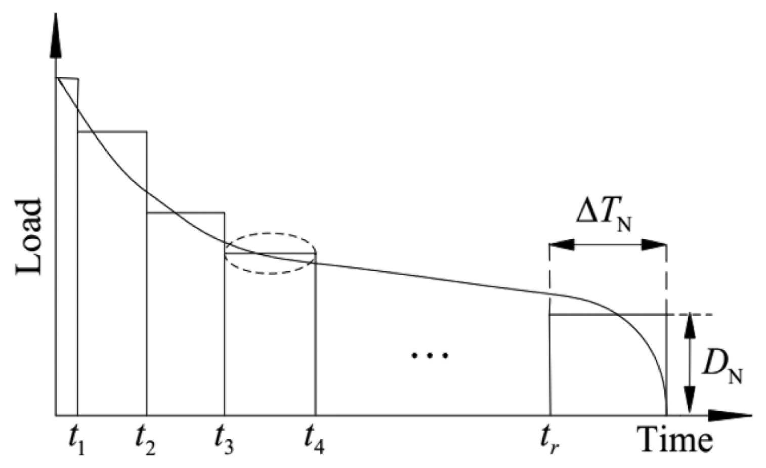
Similar to [20], the yearly load curve is approximated through a piecewise constant duration curve containing several demand blocks and shown in Figure 1.

This manifestation can be regarded as rearranging the yearly time sequence load curve into a quantity descending sequence, and merging periods with similar load levels into a single demand block. This approach is appropriate for a long term policy making problem. However, this modeling usually does not allow accurately representing time coupled operating constraints such as minimum up/down time constraints and ramping constraints of conventional units.

2.2. Bilevel Optimization Model

The parameters and variables used in the model are defined as follows:

• Parameters

  • b_i Equivalent production cost of unit i(CNY/MWh)

  • e_i Carbon emission coefficient of unit i(kg/MWh)

  • $P_i^l$ Minimal power output of unit i (MW)

  • $P_i^u$ Maximal power output of unit i (MW)

  • D_j Power consumed in demand block j(MW)

  • E_p Permitted amount of carbon emission (kg)

  • ΔT_j Time duration of demand block j(h)

• Variables

  • d_i Carbon tax rate of unit i(CNY/kg)

  • P_ij Output power of unit i in block j(MW)

The tax policy making problem can be formulated as a bilevel optimization, and regarded as a Stackelberg game, in which the government is the leader, whose strategy is the tax rate, and ISO is the follower, whose strategy is the output of generators. The upper-level (UL, the leader's problem) represents the tax rate decision process of the government agency with the target of minimizing the total levied tax subject to restricting the emission within a certain level. The lower-level (LL, the follower's problem) represents the ISO's ED problem subject to operating constraints with the tax rate fixed. The bilevel optimization model is provided as follows:

$${min}_{{\mathrm{\Delta }}^{\text{UL}}\cup {\mathrm{\Delta }}_j^{\text{LL}},\forall j}{\sum }_j{\sum }_i\mathrm{\Delta }{T}_j{d}_i{e}_i{P}_{ij}$$

(1a)

$$\text{subject to}0\le d_i\le d_i^m,\forall i$$

(1b)

$${\sum }_j{\sum }_i\mathrm{\Delta }{T}_j{e}_i{P}_{ij}\le E_p$$

(1c)

$$\text{where}{P}_{ij}\in arg\{$$

$${min}_{{\mathrm{\Delta }}_j^{\text{LL}}}{\sum }_i(b_i+d_i{e}_i)P_{ij}$$

(2a)

$$\text{subject to}{P}_i^l\le P_{ij}\le P_i^u:{\eta }_{ij}^l,{\eta }_{ij}^u,\forall i$$

(2b)

$${\sum }_i{P}_{ij}=D_j:{\mu }_j$$

(2c)

$$\}\forall j$$

where Δ^UL = {d_i,∀i}, ${\mathrm{\Delta }}_j^{\text{LL}}=\{P_{ij},{\eta }_{ij}^l,{\eta }_{ij}^u,{\mu }_j,\forall i\}$. Note that in the lower-level problems (2), dual variables are provided at the right side of their corresponding constraints following a colon, they are also decision variables following the paradigm of complementarity modeling approach [21].

The UL problem represents the total tax minimization for the government, constrained by: (i) tax rate bound (Equation (1b); (ii) carbon emission limit (Equation (1c)); (iii) a set of LL problems (Equations (2a)–(2c)). The tax rates determined in the UL problem will affect the power production of each unit in the LL problems. The ED problem minimizes the production cost of each demand block, subject to generation limits (Equation (2b)) and power balance condition (Equation (2c)). It decides the electricity generation of each unit, which in turn influences the quantity of total emission concerned by the government. The interaction between the government and the GENCOs constitutes a Stackelberg competition, in which the government is the leader, and the ISO is the follower. At the optimal solution, for the government, the target of emission reduction can be fulfilled with least additional tax. For the energy industry, the production cost is minimized subject to the given tax rate. From a game theoretical point of view, the optimal solution { $d_i^{*}$, $P_{ij}^{*}$, ∀i,j} renders a Stackelberg equilibrium, i.e.:

$${\sum }_j{\sum }_i\mathrm{\Delta }{T}_j{d}_i^{*}{e}_i{P}_{ij}^{*}\le {\sum }_j{\sum }_i\mathrm{\Delta }{T}_j{d}_i{e}_i{P}_{ij}^{*},\forall \{d_i\}\in \{d_i|0\le d_i\le d_i^m,\forall i,{\sum }_j{\sum }_i\mathrm{\Delta }{T}_j{e}_i{P}_{ij}^{*}\le E_p\}$$

where { $P_{ij}^{*}$} satisfies:

$$\left\{{\sum }_i(b_i+d_i^{*}{e}_i)P_{ij}^{*}\le {\sum }_i(b_i+d_i^{*}{e}_i)P_{ij},\forall \{P_{ij}\}\in \{P_{ij},\forall i|P_i^l\le P_{ij}\le P_i^u,\forall i,{\sum }_i{P}_{ij}=D_j\}\right\},\forall j$$

It should be pointed out that:

• In the UL problem, the tax rate may vary among different units. This setting provides more flexibility and economic superiority than using an equal tax rate on all generators. To see this, adding the constraint d₁ = d₂ = … = d_n to constraint (1b), the tax rate will be equal at the optimal solution. Consequently, because the feasible region becomes smaller, so the optimal value will be higher. In short, allowing the tax rate to vary according to different emission performance provides flexible and economical means to control emission effectively.

• The value of E_p is released by the government. Lower E_p represents more strict restriction on carbon emission. Higher E_p relaxes the emission limitations and gives priority to the economic targets.

• Because the time scale involved in the ED problem is one year, so system upgrading is not directly considered in the current formulation. To pay the tax is the only choice of generator owners. However, if long term decisions, such as the generation expansion planning decisions, are incorporated, our modeling framework is able to model long term resorts to reduce emissions under the taxation policy in the time scale of several decades rather than paying the tax, such as upgrading the generation equipment, investment on new technologies and renewable energies can be incorporated. This will lead to a different formulation of the decision problem, but the solution method directly applies. It is a very interesting topic that we are still working on.

• Direct Current (DC) power flow constraints also can be imposed in the LL ED problem to prevent transmission congestions.

• As for the objective function (2a), because the prices of the electricity is constant in China, so the income of the energy industry will also be a constant provided the total demand is fixed, namely maximizing profits is equivalent to minimizing costs. In a competitive market environment, the profit, which will be the difference of income and cost, can be used as the objective function of ED.

• It's important to restrict the cost coefficient (b_i + d_ie_i) in the objective (2a) different for each generator in order to avoid a degenerate ED problem in which the linear independent constraint qualification is not satisfied (the optimal solution is not unique). This can be implemented via several means. The simplest way is to add small disturbance on each (b_i + d_ie_i) in the ED problem, or impose the “alldifferent” constraint provided by YALMIP [22] on {b_i + d_ie_i}, ∀i. It should be pointed out that the “alldifferent” command produces additional binary variables in the final model, and may increase the computational complexity.

2.3. Equivalent Single Level Problem

As analyzed before, the UL problem (1) and the collection of LL problems (2) are interacted with each other, they should be solved simultaneously. To use off-the-shelf solvers, it's necessary to convert the bilevel model (1)–(2) into a single level optimization problem by replacing the LL problem with its first order optimality condition. Because the LL problem appears to be a linear program (LP) when the tax rate is fixed, two options are available for this task: the KKT formulation and the primal-dual formulation [23,24]. In this paper, the former is adopted because the strong duality condition will be used to linearize the nonlinear objective function (1a) following the method presented in [21,25,26].

Note that for fixed tax rates, the LL problems (2) are LPs and decoupled with respect to block j, their corresponding KKT conditions are as follows:

$$\begin{array}{c}{b}_i+d_i{e}_i+{\eta }_{ij}^u-{\eta }_{ij}^L-\mathbf{1}{\mu }_j,\forall i\\ {\sum }_i{P}_{ij}=D_j\\ 0\le P_{ij}-P_i^l\perp {\eta }_{ij}^l\ge 0,\forall i\\ 0\le P_i^u-P_{ij}\perp {\eta }_{ij}^u\ge 0,\forall i\end{array}\}\forall j$$

(3)

where the expression “ $a\perp b$ ” means at most one of a and b can take a strictly positive value, while the other being at 0. So problem (1)–(2) becomes:

$$min{\sum }_j{\sum }_i\mathrm{\Delta }{T}_j{d}_i{e}_i{P}_{ij}$$

(4a)

$$\text{subject to}0\le d_i\le d_i^m,\forall i$$

(4b)

$${\sum }_j{\sum }_i\mathrm{\Delta }{T}_j{e}_i{P}_{ij}\le E_p$$

(4c)

$$b_i+d_i{e}_i+{\eta }_{ij}^u-{\eta }_{ij}^L-\mathbf{1}{\mu }_j,\forall i,j$$

(4d)

$${\sum }_i{P}_{ij}=D_j,\forall j$$

(4e)

$$0\le P_{ij}-P_i^l\perp {\eta }_{ij}^l\ge 0,\forall i,j$$

(4f)

$$0\le P_i^u-P_{ij}\perp {\eta }_{ij}^u\ge 0,\forall i,j$$

(4g)

However, problem (4) is instinctively hard to solve because the Mangasarian-Fromovitz constraint qualification fails at every feasible point [27] due to the presence of the complementarity and slackness conditions in Equations (4f) and (4g). Moreover, the objective function in Equation (4a) is bilinear and thus non-convex, it's difficult to retrieve a global optimal solution. In the next section, problem Equation (4) will be transformed into an equivalent MILP whose global optimum can be solved efficiently by state-of-the-art MILP solvers.

3. Solution of the Bilevel Model

The single level optimization problem (4) includes two kinds of nonlinearities:

(1)

the complementarity and slackness conditions in (4f) and (4g);

(2)

the bilinearity in the objective function (4a);

They are subsequently linearized in the following two subsections.

3.1. Linearizing the Complementarity Constraints

The complementarity and slackness conditions in (4f) and (4g) can be linearized by introducing auxiliary binary variables $z_{ij}^l$ and $z_{ij}^u$, and replacing them with following disjunctive constraints [28]:

$$0\le P_{ij}-P_i^l\le M{z}_{ij}^l,\forall i,j$$

(5a)

$$0\le {\eta }_{ij}^l\le M(1-z_{ij}^l),\forall i,j$$

(5b)

$$0\le P_i^u-P_{ij}\le M{z}_{ij}^u,\forall i,j$$

(5c)

$$0\le {\eta }_{ij}^u\le M(1-z_{ij}^u),\forall i,j$$

(5d)

where M is a conceptual large enough constant. If M is properly chosen, it can be seen from Equations (5a)–(5b) that at most one of $\{P_{ij}-P_i^l,{\eta }_{ij}^l\}$ can take a strictly positive value, because $z_{ij}^l$ is binary. It should be noticed that the value of M must be selected carefully. If M is too small, constraint (5) will impose smaller bounds to the original model [29]. In contrast, if M is too large, the resulting problem will be ill-condition and difficult to converge [24]. There is no universal method to select an appropriate value of M for an arbitrary model. This paper gives a heuristic way to determine proper bounds of dual variables based on the physical interpretation of Lagrange multipliers.

Variables ${\eta }_{ij}^u$ can be regarded as the sensitivity of the objective function (2a) with respect to the right hand side term $P_i^u$. Suppose that $P_i^u$ is changed to $P_i^u+\mathrm{\Delta }{P}_i^u$, the original optimal value f of LL problem (2) is consequently changed to f + Δf. The incremental cost Δf can be interpreted as follows: the output of unit i increases $\mathrm{\Delta }{P}_i^u$, according to the power balance condition (2c), there must be some other unit decreases its output by $\mathrm{\Delta }{P}_i^u$, so the change in the objective function Δf satisfies:

$$|\mathrm{\Delta }f|\le |{max}_j(d_i-d_j)\mathrm{\Delta }{P}_i^u|$$

As a result:

$${\eta }_{ij}^u\le |{max}_j\{d_i-d_j\}|\le {max}_j\{d_j\}$$

The same procedure can be applied to drive the bound of ${\eta }_{ij}^l$. So the parameter M in Equations (5b) and (5d) can be selected as:

$$M={max}_j\{d_j\}$$

(6)

The value of M for Equations (5a) and (5c) with primal variables can be simply selected as:

$$M={max}_j\{P_i^u\}$$

(7)

To sum up, M should be selected as:

$$M=max\{{max}_j\{P_i^u\},{max}_j\{d_j\}\}$$

(8)

3.2. Linearizing the Objective Function

The bilinearity in the objective function (4a) can be linearized following the method presented in [21,25,26]. According to the strong duality theorem of LP, the objective functions of a primal LP and its corresponding dual LP takes the same value at the optimum. Thus the following equality holds for LL problem (2):

$${\sum }_i(b_i+d_i{e}_i)P_{ij}=-{\mu }_j{D}_j+{\sum }_i{P}_i^u{\eta }_{ij}^u-{\sum }_i{P}_i^l{\eta }_{ij}^l,\forall j$$

(9)

Thus:

$${\sum }_i{d}_i{e}_i{P}_{ij}={\sum }_i{P}_i^u{\eta }_{ij}^u-{\sum }_i{P}_i^l{\eta }_{ij}^l-{\mu }_j{D}_j-{\sum }_i{b}_i{P}_{ij},\forall j$$

(10)

Substituting Equation (10) into Equation (4a) yields:

$${\sum }_j{\sum }_i\mathrm{\Delta }{T}_j{d}_i{e}_i{P}_{ij}={\sum }_j\mathrm{\Delta }{T}_j({\sum }_i{P}_i^u{\eta }_{ij}^u-{\sum }_i{P}_i^l{\eta }_{ij}^l-{\mu }_j{D}_j-{\sum }_i{b}_i{P}_{ij})$$

(11)

The right hand side of Equation (11) is linear in variables ${\eta }_{ij}^l$, ${\eta }_{ij}^u$, μ_j and P_ij.

3.3. The Final MILP

In model (4), replacing the objective function (4a), constraint (4f) and (4g) with Equations (11) and (5), respectively, renders the following MILP:

$$min{\sum }_j{\sum }_i\mathrm{\Delta }{T}_j({\sum }_i{P}_i^u{\eta }_{ij}^u-{\sum }_i{P}_i^l{\eta }_{ij}^l-{\mu }_j{D}_j-{\sum }_i{b}_i{P}_{ij})$$

(12a)

subject to:

$${\sum }_j{\sum }_i\mathrm{\Delta }{T}_j{e}_i{P}_{ij}\le E_p$$

(12b)

$$d_i\ge 0,\forall i$$

(12c)

$${\sum }_i{P}_{ij}=D_j,\forall j$$

(12d)

$$b_i+d_i{e}_i+{\eta }_{ij}^u-{\eta }_{ij}^L-\mathbf{1}{\mu }_j,\forall i,j$$

(12e)

$$0\le P_{ij}-P_i^l\le M{z}_{ij}^l,\forall i,j$$

(12f)

$$0\le {\eta }_{ij}^l\le M(1-z_{ij}^l),\forall i,j$$

(12g)

$$z_{ij}^l\in \{0,1\},\forall i,j$$

(12h)

$$0\le P_i^u-P_{ij}\le M{z}_{ij}^u,\forall i,j$$

(12i)

$$0\le {\eta }_{ij}^u\le M(1-z_{ij}^u),\forall i,j$$

(12j)

$$z_{ij}^u\in \{0,1\},\forall i,j$$

(12k)

where the parameter M is selected according to Equation (8).

4. Case Study

To validate the effectiveness of the proposed model and algorithm, numeric experiments on a 10-unit system and a provincial power grid in China are carried out. YALMIP is used to formulate the model. CPLEX 12.2 is used to solve related MILP problems.

4.1. 10-Unit System

The parameters of generators and demand blocks of the 10-unit system are given in

Table 1. Parameters of generators.

Unit	$P_I^u$ (MW)	$P_i^l$ (MW)	b (CNY/MWh)	e (kg/MWh)
G1	1000	600	554	1004.7
G2	840	350	536	1034.0
G3	700	300	518	1063.3
G4	660	200	540	1096.3
G5	600	200	445	1114.7
G6	500	150	400	1129.3
G7	450	150	372	1169.7
G8	450	150	330	1140.3
G9	300	100	346	1191.7
G10	100	50	320	1257.7

and

Table 2. Parameters of load blocks.

Block	Demand (MW)	Duration (h)
1	5000	1000
2	4500	3000
3	4000	3000
4	3500	1000
5	3000	760

, respectively.

In the 10-unit system, the parameters of generators are collected from typical generators in China. Each generator has a coal consumption rate c_i measured from operating data. The carbon emission coefficient e_i = 44c_i/12, because the molecular weight of carbon and CO₂ is 12 and 44, respectively, this means burning 1kg coal produces 44/12 kg CO₂. As for the parameters of load blocks, the demand levels are assumed according to the capacity of generators, the time durations are the same as that in [20]. Note that the parameter b is the equivalent production cost of generators, which depends on multiple factors, such as the pure generation cost, CO₂/SO₂ capture cost, maintenance fee, repayment for the construction investment and so on. Usually, the larger plants have lower unit production costs, but higher other costs than the smaller ones, especially the repayment during the first decade since it is built. So in a period of a few years, b_i may be higher for larger generators. Nevertheless, this is not a universal law. In the next case of the Guangdong power grid, some large generators have lower b_i than smaller ones.

In this case, the parameter E_p is determined through two optimization problems. First, the optimal production cost problem (13) is solved. The optimal value is C_min, and the corresponding carbon emission is E_max:

$$min{\sum }_j{\sum }_i\mathrm{\Delta }{T}_j{b}_i{P}_{ij}$$

(13a)

$$s.t.P_i^l\le P_{ij}\le P_i^u,\forall i,j$$

(13b)

$${\sum }_i{P}_{ij}=D_j,\forall j$$

(13c)

Then the optimal emission problem (14) is solved. The optimal value is E_min and the corresponding production cost is C_max. The results of problem (13) and (14) with respect to the considered system are shown in

Table 3. Optimal cost and emission.

Optimal production cost problem		Optimal emission problem
Cmin (CNY)	Emax (kg)	Cmax (CNY)	Emin (kg)
1.6352 × 1010	3.9941 × 1010	1.8149 × 1010	3.8775 × 1010

:

$$min{\sum }_j{\sum }_i\mathrm{\Delta }{T}_j{e}_i{P}_{ij}$$

(14a)

$$s.t.P_i^l\le P_{ij}\le P_i^u,\forall i,j$$

(14b)

$${\sum }_i{P}_{ij}=D_j,\forall j$$

(14c)

The value of E_p is chosen between E_min and E_max as follows:

$$E_p=\alpha E_{min}+(1-\alpha )E_{max},0\le \alpha \le 1$$

(15)

The optimal tax rate under different permitted emission level α is computed from MILP (12) and shown in

Table 4. Optimal tax rate under different permitted emission level.

Unit	Optimal tax rate (CNY/kg)
	α = 0.2	α = 0.4	α = 0.6	α = 0.8	α = 1.0
G1	0	0	0	0	0
G2	0	0	0	0	0.0674
G3	0	0	0.1310	0	0.1310
G4	0.0502	0.0502	0.0502	0.0502	0.0569
G5	0	0.3651	0	0.3651	0.3717
G6	0	0	0	0.5097	0.5162
G7	0	0	0.5799	0.5831	0.5925
G8	0	0	0	0	0.7395
G9	0.6462	0.6492	0.6523	0.6554	0.6646
G10	0	0	0.6968	0	0.7085

.

From Table 4 we can see, in general, generators with larger emission rate will be levied higher tax, which coincides with our intuition, but it's not necessary that high emission generators should always be taxed with high priority because their capacity may be small thus has less impact on the quantity of emission.

With the optimal tax rates fixed, the LL ED problem is solved. The production cost (∑_j∑_iΔT_jb_iP_ij), the total tax cost (∑_j∑_iΔT_jd_ie_iP_ij), the permitted amount of carbon emission E_p (defined in Equation (15)) and the expected emission (∑_j∑_iΔT_je_iP_ij) are shown in

Table 5. Production cost and emission under different permitted emission level.

Emission level	Cost (108 CNY)		Emission (1010 kg)
	Production	Tax	Permitted	Expected
α = 0.2	166.39	2.1114	3.9706	3.9692
α = 0.4	169.31	4.1249	3.9472	3.9450
α = 0.6	171.98	6.9378	3.9241	3.9233
α = 0.8	176.64	10.242	3.9006	3.8991
α = 1.0	181.49	20.370	3.8775	3.8775

. The total electricity generated by each unit is shown in

Table 6. Electricity generated by each unit under different permitted emission level.

Unit	Quantity of electricity production (GWh)
	α = 0.2	α = 0.4	α = 0.6	α = 0.8	α = 1.0
G1	5656	6736	7486	8066	8760
G2	4906	6076	6696	6986	7252
G3	5278	5678	2978	6132	5788
G4	1812	2212	3142	3922	4972
G5	4802	1752	5028	2602	3352
G6	4190	4190	4380	1564	1964
G7	3942	3942	1314	1314	1314
G8	3942	3942	3942	3942	1564
G9	876	876	876	876	876
G10	876	876	438	876	438

.

From Table 5, it can be seen that the expected emission corresponding to the optimal dispatch decision of the ISO is always less than that it is allowed. This important feature demonstrates the bilevel model endows the carbon tax scheme an indirect but effective control ability on the quantity of emission. Meanwhile, the tax cost is 1.3%–4% of the production cost when α varies from 0.2 to 0.6, which is relative reasonable, namely the profit of GENCOs will not be dramatically influenced even the selling price does not change. From Table 6, it's easily concluded that low emission generators produce more electricity with E_p decreasing (α increasing).

4.2. Guangdong Power Grid of China

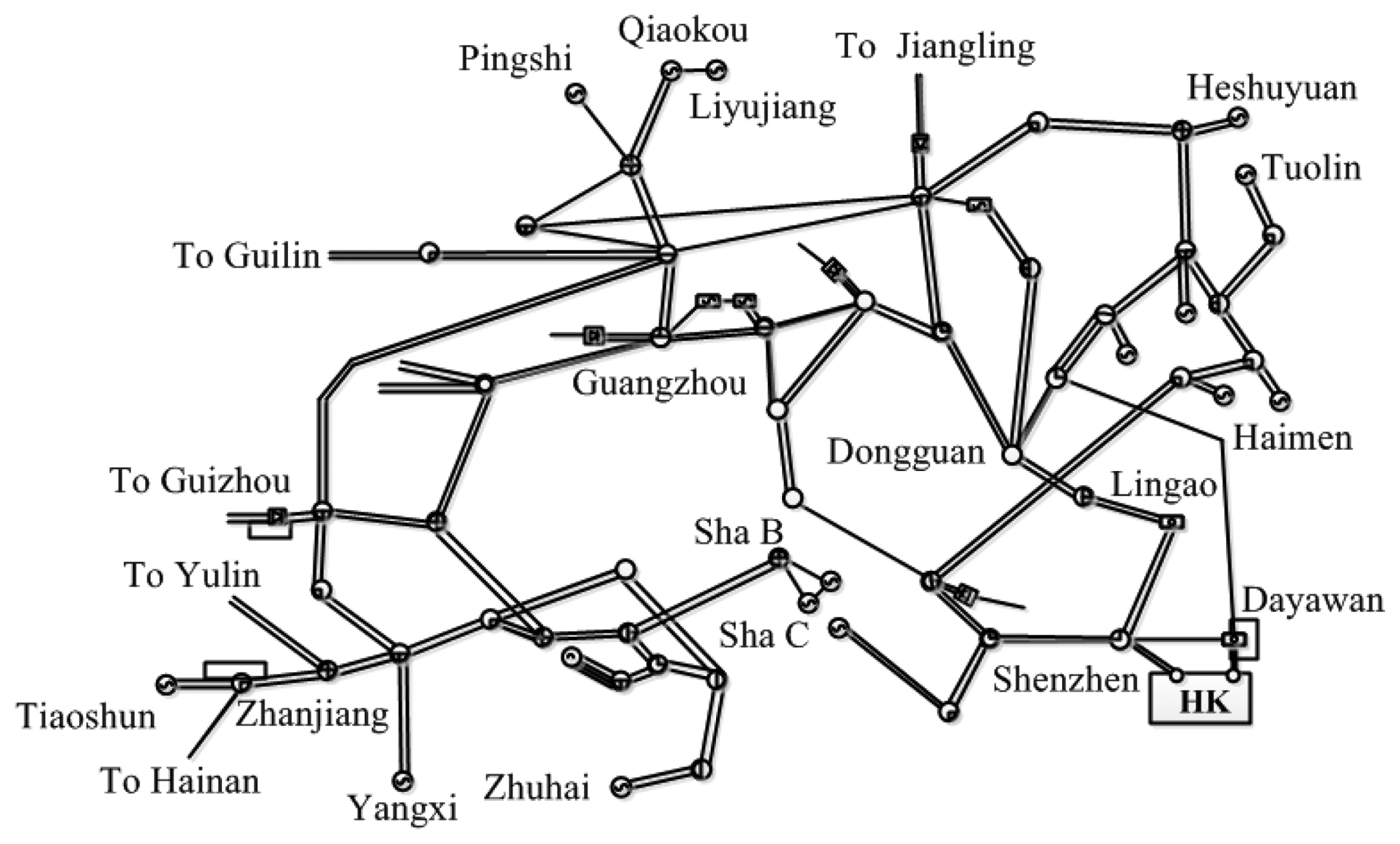
The realistic Guangdong power grid of China is studied in this case. One hundred and seventy four (174) generating units with a total 58,744 MW capacity are available in this system. The topology of the 500 kV main transmission network is shown in Figure 2. The parameters of demand blocks are given in

Table 7. Load blocks of the Guangdong power grid.

Block	Demand (MW)	Duration (h)
1	55,805	1,000
2	49,931	3,000
3	44,056	3,000
4	38,182	1,000
5	35,245	760

.

In this system, it's found that some generators in the same power plant have identical parameters. To simplify the bilevel model (1)–(2) and reduce binary variables in MILP (12), generators with the same cost coefficient b_i and carbon emission coefficient e_i are aggregated into a single equivalent one whose minimal output $P_i^l$ /maximal output $P_i^u$ is the sum of all generators to be aggregated, while b_i and e_i remain the same. For example, there are three generators whose production cost coefficients b = 500 CNY/MWh, carbon emission coefficient e = 1050 kg/MWh, the capacity parameter is $P_1^u=P_2^u=600\text{MW}$, $P_1^l=P_2^l=300\text{MW}$ and $P_3^u=800\text{MW}$, $P_3^l=400\text{MW}$, respectively, then the aggregated generator's parameters are b = 500 CNY/MWh, e = 1050 kg/MWh, P^u = 2000 MW, P^l = 1000 MW, respectively. Using this equivalence, 52 aggregated generators remain in the system.

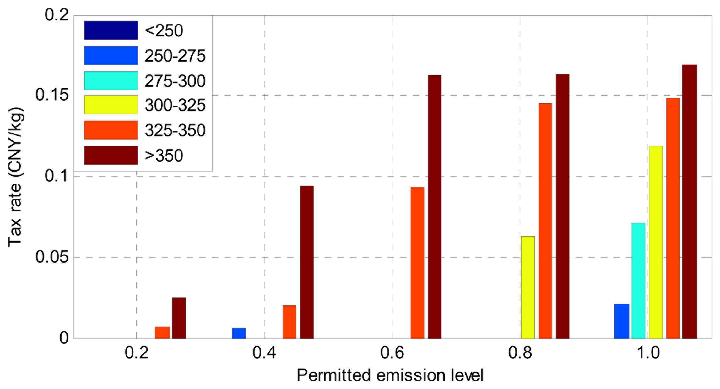
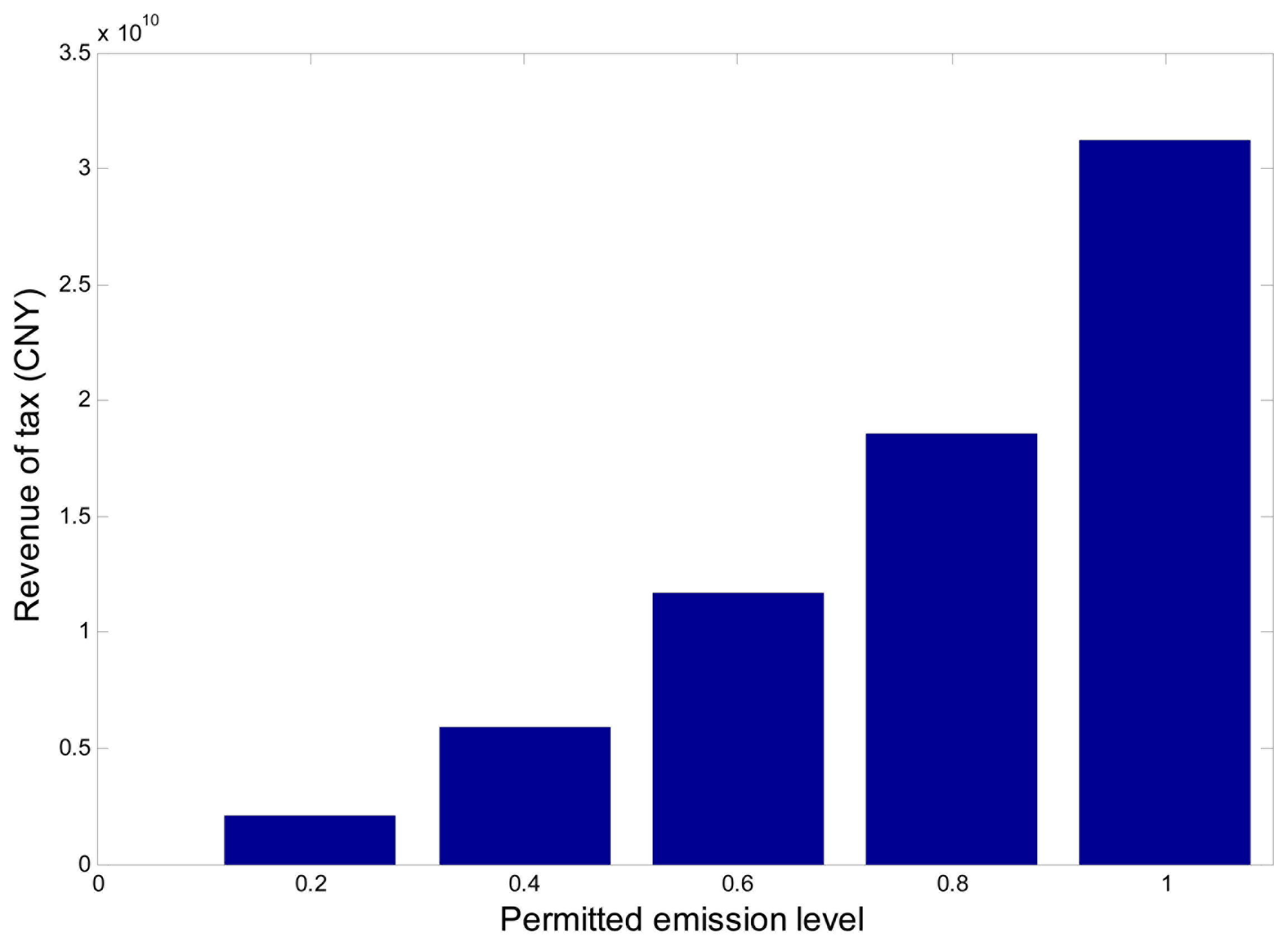
It's also found that the equivalent production costs of most new-built generators with CO₂/SO₂ capture facilities are usually higher than the old ones without advanced environmental protection equipment. Therefore, a traditional cost-minimized energy scheduling scheme will result in higher emissions. If carbon tax is imposed on Guangdong power grid, bilevel model (1)–(2) is used to study how to determine an appropriate tax rate among generating units. The results are shown through Figures 3, 4 and 5. The permitted amount of carbon emission E_p is chosen using the same method proposed in the previous subsection, and characterized by the parameter α. In practice, the National Development and Reform Commission of China, or the Southern Power Grid Company of China is responsible to release the parameter E_p for Guangdong power grid.

According to our modeling method, each aggregated unit has a corresponding optimal tax rate for a fixed permitted emission level. To illustrate them clearly, the 52 aggregated generators are divided into 6 groups. Each group contains a number of aggregated generators whose coal consumption rate is within a certain range. The coal consumption interval of each group is given in

Table 8. Coal consumption interval of each group (kg/MWh).

Type of bound	Group 1	Group 2	Group 3	Group 4	Group 5	Group 6
Lower bound	0	250	280	300	320	350
Upper bound	250	280	300	320	350	398

. The carbon emission coefficient e_i is 44/12 times the corresponding coal consumption rate.

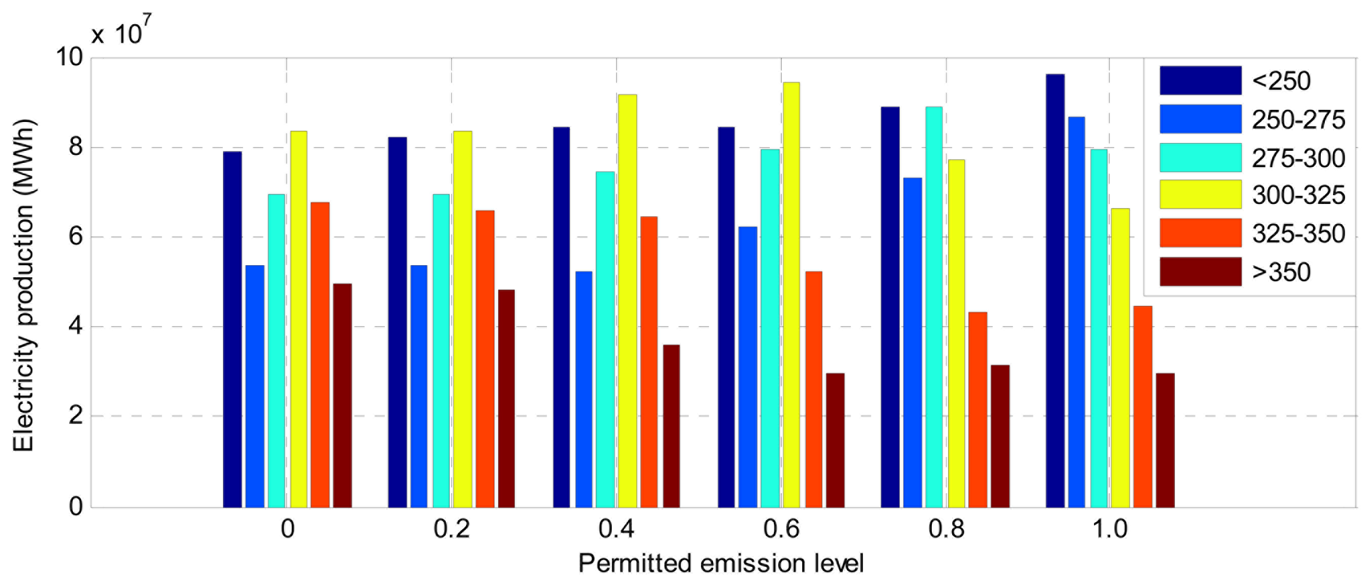
Figures 3 and 4 show the weighted average tax rate and total electricity production of each group under different permitted emission level, respectively. They are calculated as follows:

$$\begin{array}{ll}{\text{Tax}}_I^G=\frac{{\sum }_{i\in \text{Group}(I)}{P}_i^u{d}_i}{{\sum }_{i\in \text{Group}(I)}{P}_i^u},\hfill & {\text{Electricity}}_I^G={\sum }_j{\sum }_{i\in \text{Group}(I)}{P}_{ij}\mathrm{\Delta }{T}_j\hfill \end{array}$$

(16)

From Figures 3 and 4 we can see, to reduce carbon emission, a carbon tax is usually priorly levied on the generators with high coal consumption level. As a result, the electricity produced by such units is reduced. To meet the load demand, low-emission units generate more electricity, so the total emission decreases, at the cost of increasing the funds to pay.

The permitted amount of carbon emission E_p and expected emission (∑_j∑_iΔT_je_iP_ij) is compared in

Table 9. Comparison of the permitted emission and expected emission.

Emission level	Emission (1011 kg)
	Permitted	Expected
α = 0.2	3.8491	3.8491
α = 0.4	3.8074	3.8071
α = 0.6	3.7656	3.7654
α = 0.8	3.7239	3.7238
α = 1.0	3.6822	3.6822

. It is verified that the expected emission is always no more than it is allowed. In other words, the pre-specified emission gives a valid upper bound if the production cost is minimized at the lower level. Because the optimal solution of ED happens at one vertex of its feasible polyhedron, the actual emission is not continuous. Therefore, in Table 9 (as well as in Table 5) there is slight difference between the permitted emission and expected emission.

Finally, Figure 5 shows the total tax (∑_j∑_iΔT_jd_ie_iP_ij) levied from Guangdong power grid under different permitted emission levels. If a “unit cost of carbon emission” is defined as follows:

$$C_U=\frac{{\sum }_j{\sum }_i\mathrm{\Delta }{T}_j{d}_j^{*}{e}_j{P}_{ij}^{*}}{E_p-E_{min}}$$

(17)

where $d_j^{*}$ and $P_{ij}^{*}$ is the optimal tax rate and energy offer under the permitted emission level. It's found that C_U increases with the permitted emission level α increasing.

5. Conclusions

This paper presents a bilevel optimization model for the carbon emission taxing problem that can strike a proper balance between the target of emission reduction and the profit of emission sectors. The model is finally converted into a tractable MILP without any approximation and can be efficiently solved by commercial solvers. Our model possesses two distinguished features: (1) The Stackelberg competition between the tax maker and emission sectors under regulation is explicitly modeled; (2) The actual emission corresponding to the optimal ED solution is no more than the pre-specified value.

It's found in the case studies that: (1) according to the design parameters and operating data of typical generators in China, generators with higher emission coefficients will generally have higher tax rates; (2) the unit cost of carbon emission increases with the decreasing permitted emissions, but the total tax is still within a reasonable range when α varies from 0.2 to 0.6. These results provide practical references for relevant government agencies.

Further work will be focused on extending the proposed formulation to a generation expansion planning framework, thus upgrading the generation equipment, investment on new technologies and renewable energies could be modeled. If the uncertainty resulting from long term decisions and renewable generation is considered, the problem will be more challenging and worthy of studying.

References

- Le Treut, H.; Somerville, R.; Cubasch, U.; Ding, Y.; Mauritzen, C.; Mokssi, A.; Peterson, T.; Prather, M. In Historical Overview of Climate Change, Climate Change: The Physical Science Basis; Contribution of Working Group I to the Fourth Assessment Report of the Intergovernmental Panel on Climate Change. Cambridge University Press: Cambridge, UK; New York, NY, USA, 2007. [Google Scholar]
- Stavins, R.N. Market-based environmental policies. Publ. Pol. Environ. Protect. 2000, 2, 31–76. [Google Scholar]
- Stavins, R.N. Experience with market-based environmental policy instruments. Handb. Environ. Econ. 2003, 1, 355–435. [Google Scholar]
- Carbon Tax and Greenhouse Gas Control: Options and Considerations for Congress. Available online: https://www.fas.org/sgp/crs/misc/R40242.pdf (accessed on 10 November 2013).
- Denny, E.A.; Buchner, B.K. The European Union emissions trading scheme: Origins, allocation, and early results. Rev. Environ. Econ. Policy 2007, 1, 66–87. [Google Scholar]
- Mansanet-Bataller, M.; Pardo, Á. What you should know about carbon markets. Energies 2008, 1, 120–153. [Google Scholar]
- Considine, T.; Larson, D.F. Short term electric production technology switching under carbon cap and trade. Energies 2012, 5, 4165–4185. [Google Scholar]
- Metz, B. In Climate Change 2001: Mitigation; Contribution of Working Group III to the Third Assessment Report of the Intergovernmental Panel on Climate Change. Cambridge University Press: Cambridge, UK; New York, NY, USA, 2011. [Google Scholar]
- Huang, Y.H.; Wu, J.H. Energy policy in Taiwan: Historical developments, current status and potential improvements. Energies 2009, 2, 623–645. [Google Scholar]
- Szlavik, J.; Csete, M. Climate and energy policy in Hungary. Energies 2012, 5, 494–517. [Google Scholar]
- Keohane, N. Cap and trade, rehabilitated: Using tradable permits to control U.S. greenhouse gases. Rev. Environ. Econ. Policy 2009, 3, 42–62. [Google Scholar]
- Johnson, K. A decarbonization strategy for the electricity sector: New-source subsidies. Energy Policy 2010, 38, 2499–2507. [Google Scholar]
- Metcalf, G. Designing a carbon tax to reduce US greenhouse gas emissions. Rev. Environ. Econ. Policy 2009, 3, 63–83. [Google Scholar]
- He, Y.; Wang, L.; Wang, J. Cap-and-trade vs. carbon taxes: A quantitative comparison from a generation expansion planning perspective. Comput. Ind. Eng. 2012, 63, 708–716. [Google Scholar]
- Liu, Y.; Huang, G.; Cai, Y.; Dong, C. An inexact mix-integer two-stage linear programming model for supporting the management of a low-carbon energy system in China. Energies 2011, 4, 1657–1686. [Google Scholar]
- Chen, D.; Gong, Q.; Zou, B.; Zhang, X.; Zhao, J. A low-carbon dispatch model in a wind power integrated system considering wind speed forecasting and energy-environmental efficiency. Energies 2012, 5, 1245–1270. [Google Scholar]
- Tan, X.C.; Wang, Y.Y.; Gu, B.H.; Mu, Z.K.; Yang, C. Improved methods for production manufacturing processes in environmentally benign manufacturing. Energies 2011, 4, 1391–1409. [Google Scholar]
- Zeng, Y.; Cai, Y.; Huang, G.; Dai, J. A Review on optimization modeling of energy systems planning and GHG emission mitigation under uncertainty. Energies 2011, 4, 1624–1656. [Google Scholar]
- Li, Y.; Cui, J. A method of designing energy tax rate based on game theory. Proceedings of the 7th International Symposium on Operations Research and Its Applications (ISORA'08), Lijiang, China, 31 October–3 November 2008.
- Baringo, L.; Conejo, A.J. Transmission and wind power investment. IEEE Trans. Power Syst. 2012, 27, 885–893. [Google Scholar]
- Gabriel, S.A.; Conejo, A.J.; Hobbs, B.F.; Fuller, D.; Ruiz, C. Complementarity Modeling in Energy Markets; Springer: New York, NY, USA, 2012. [Google Scholar]
- YALMIP Online Manual. Available online: http://users.isy.liu.se/johanl/yalmip/ (accessed on 16 October 2013).
- Fernandez-Blanco, R.; Arroyo, J.M.; Alguacil, N. Network-constrained day-ahead auction for consumer payment minimization. IEEE Trans. Power Syst. 2014, 29, 526–536. [Google Scholar]
- Ruiz, C.; Conejo, A.J.; Smeers, Y. Equilibria in an oligopolistic electricity pool with stepwise offer curves. IEEE Trans. Power Syst. 2012, 27, 752–761. [Google Scholar]
- Baringo, L.; Conejo, A.J. Strategic offering for a wind power producer. IEEE Trans. Power Syst. 2013, 28, 4645–4654. [Google Scholar]
- Kazempour, S.J.; Conejo, A.J.; Ruiz, C. Strategic generation investment using a complementarity approach. IEEE Trans. Power Syst. 2011, 26, 940–948. [Google Scholar]
- Scheel, H.; Scholtes, S. Mathematical programs with complementarity constraints: Stationarity, optimality, and sensitivity. Math. Oper. Res. 2000, 25, 1–22. [Google Scholar]
- Fortuny-Amat, J.; McCarl, B. A representation and economic interpretation of a two-level programming problem. J. Oper. Res. Soc. 1981, 32, 783–792. [Google Scholar]
- Ruiz, C.; Conejo, A.J. Pool strategy of a producer with endogenous formation of locational marginal prices. IEEE Trans. Power Syst. 2009, 24, 1855–1866. [Google Scholar]