Failure Test and Finite Element Simulation of a Large Wind Turbine Composite Blade under Static Loading

Abstract
: This study presented a failure analysis of a 52.3 m composite wind turbine blade under static loading. Complex failure characteristics exhibited at the transition region of the blade were thoroughly examined and typical failure modes were indentified. In order to predict multiple failure modes observed in the tests and gain more insights into the failure mechanisms of the blade, a Finite Element (FE) simulation was performed using a global-local modeling approach and Progressive Failure Analysis (PFA) techniques which took into account material failure and property degradation. Failure process and failure characteristics of the transition region were satisfactorily reproduced in the simulation, and it was found that accumulated delamination in spar cap and shear web failure at the transition region were the main reasons for the blade to collapse. Local buckling played an important role in the failure process by increasing local out-of-plane deformation, while the Brazier effect was found not to be responsible for the blade failure.
1. Introduction
With the expansion of wind energy in recent years, the sizes of wind turbine blades have become increasingly large in order to capture more power from wind and further reduce the cost of energy [1,2]. When blades are small tip deflection is a major driver in structural design and blade failure is of less concern. However, as blade sizes grow, the types of failure change and three-dimensional stresses become important [3]. In order to investigate the failure behavior of large blades installed on multi-megawatt (MW) wind turbines, some researchers have carried out failure tests on full-scale blades. Among them, Jorgensen, et al. [4] performed a failure test on a 25 m blade under flap-wise bending emphasizing the geometrical nonlinearity at large deflections. Jensen et al. [5–7] tested a 34 m blade and its load-carrying box girder under flap-wise bending and found that the Brazier effect induced a large deformation in the spar cap and the further delamination buckling were the cause leading to structural collapse. Overgarrd et al. [8,9] tested a 25 m blade to failure under flap-wise bending and concluded that the ultimate strength of the blade was governed by instability phenomena in the form of delamination and buckling instead of the Brazier effect. Yang et al. [10] studied the structural collapse of a 40 m blade under flap-wise bending and found that debonding of aerodynamic shells from adhesive joints was a main reason for the blade to collapse. Chou et al. [11] investigated a typhoon-damaged composite blade with a blade length close to 39.5 m and showed that the blade failed by delamination and laminate cracking. It can be seen that failure causes varied among blades and little consensus has been reached.
Although several failure incidents of 50+ m blades have been reported in recent years [12], no experimental study focused on the failure of blades with lengths longer than 40 m has been publically reported so far according to the authors' knowledge. It is considered that larger blades may exhibit more complex failure behavior which has neither been observed from the existing studies nor been paid enough attention to in current blade design. Therefore, there is an urgent need of experimental studies on large blades to gain more understanding on their failure behavior. Furthermore, numerical models capable of predicting blade failure in a large structural scale are also essential to complement experimental studies due to the expensive cost associated with full-scale blade tests. Although some researchers [13–15] have successfully investigated failure behavior of composite blades using the Finite Element (FE) method, they primarily focused on in-plane failure mode, i.e., laminate fracture (LF), for which failure criteria based on a two-dimensional stress field are readily available in most commercial FE programs. As observed from the existing failure tests on large composite blades, through-thickness failure mode in the form of delamination appears to be more crucial than the in-plane one. Only a few works, i.e., [8,9], have investigated delamination of blades numerically in a structural scale and the FE program they used was developed in-house. It is therefore of significance to develop a modeling method based on commonly used FE programs with which blade designers are familiar for predicting the failure behavior of large blades.
In order to partially meet the need of experimental and numerical studies on the failure of large blades, this study presents a full-scale failure test of a 52.3 m blade with particular focus on its complex failure characteristics which were associated with both in-plane and through-thickness failure modes and have not been investigated by other studies focusing on smaller blades. In order to predict the complex failure characteristics of the blade, this study proposes a FE modeling method based on a commercial FE program and further investigated the mechanisms leading to the blade failure. It was expected that more understanding on the failure of large wind turbine blades could be obtained from this study.
The contents of this paper are organized as follows: general information and experimental procedures of the blade were described and then failure characteristics were investigated in Section 2; in Section 3 a FE modeling method which was capable of predicting complex failure characteristics of the blade was proposed taking advantage of Progressive Failure Analysis (PFA) techniques and a global-local modeling approach; after assessing numerical models by comparing predicted structural response with available experimental measurements, failure process and failure characteristics of the blade were reproduced in Section 4; based on failure test and numerical simulation the root cause of failure and the Brazier effect were examined to understand the failure mechanisms of the blade in Section 5; finally, the findings obtained from this study are summarized in Section 6.
2. Full-Scale Failure Test
Commercial wind turbine blades have to pass full-scale tests required by blade certification bodies [16,17] in order to start a series production of those blade types. Static bending loads are applied in the test to simulate extreme wind loads the blades are expected to sustain in their design lives. This section presents general information and the experimental procedure of the blade under concern and investigated its complex failure characteristics through post-mortem observations.
2.1. General Information of the Blade
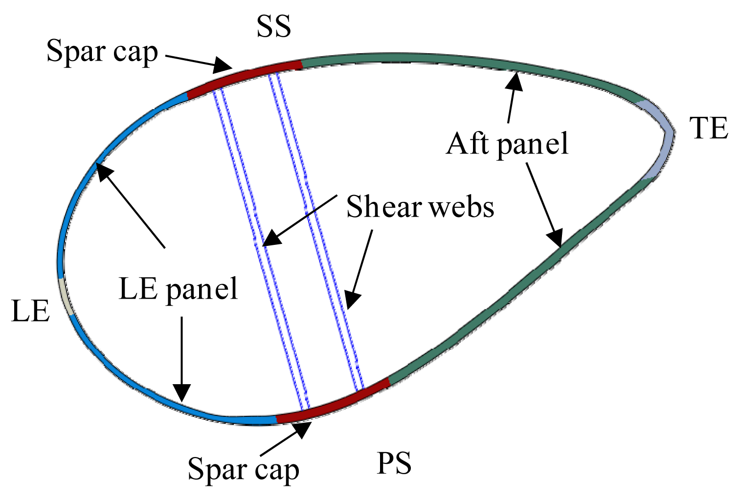
The blade was designed for 2.5 MW wind turbines and had a total length of 52.3 m. It was made of glass fabrics and vacuum infused with epoxy resin. Typical construction of the blade cross-sections is shown in Figure 1. Spar caps were made of composite laminates and designed to carry bending moments, while leading edge (LE) panel and aft panel were made of sandwich constructions with PVC foam cores and designed to provide an aerodynamic airfoil shape. Shear webs were also sandwich constructions and designed to support two spar caps and transfer shear forces.
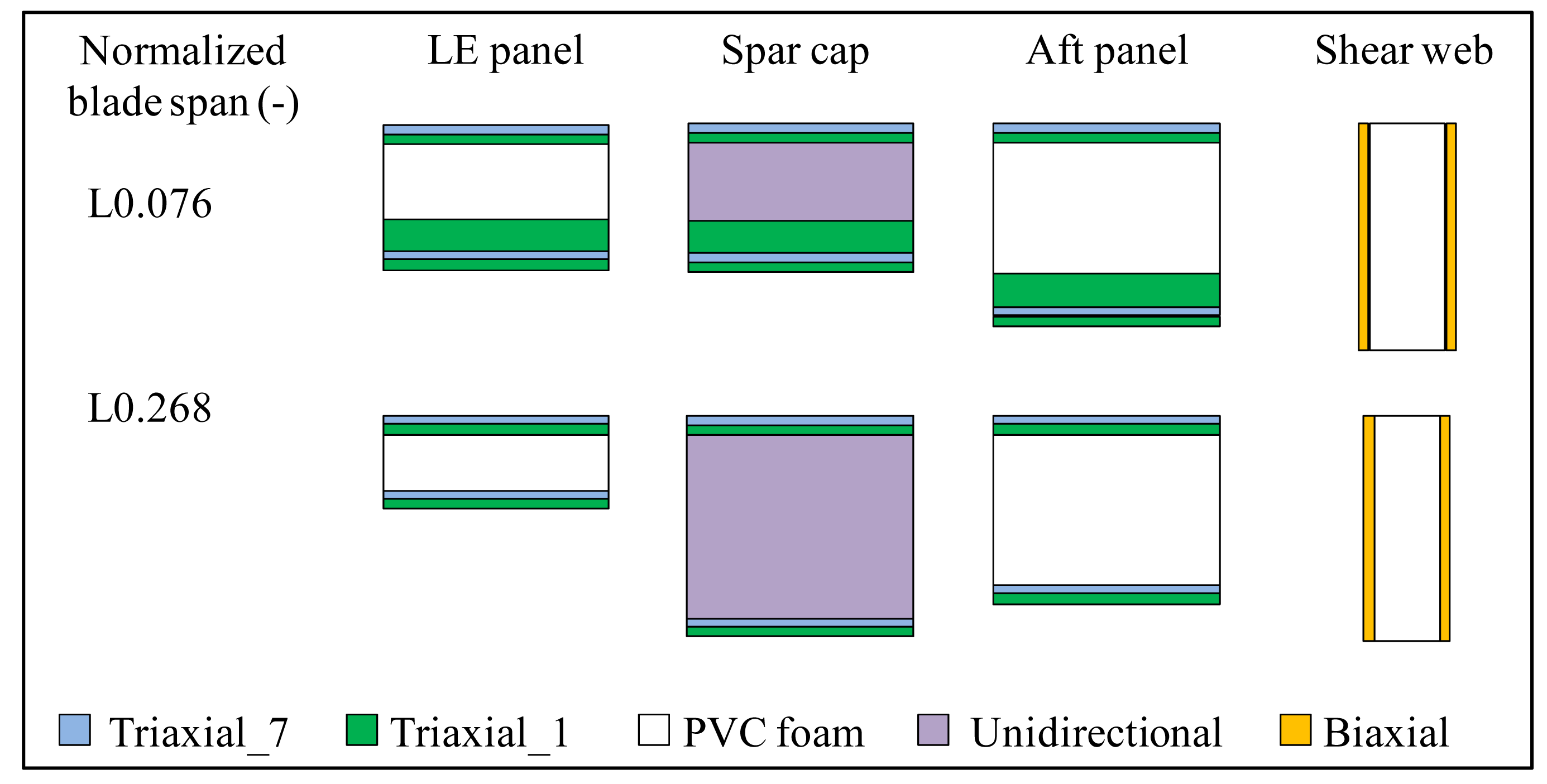
Throughout this paper span-wise locations of the blade were normalized by the total length of the blade and denoted as “Lxxxx”. For example, a span-wise location of 4 m was denoted as “L0.076” in Figure 2, which shows composite layups at representative blade locations. The blade surfaces contained two types of triaxial laminates denoted as “Triaxial_7” and “Triaxial_1”; spar caps contained a large amount of unidirectional laminates and shear webs contained biaxial laminates as sandwich skins.
2.2. Experimental Procedure
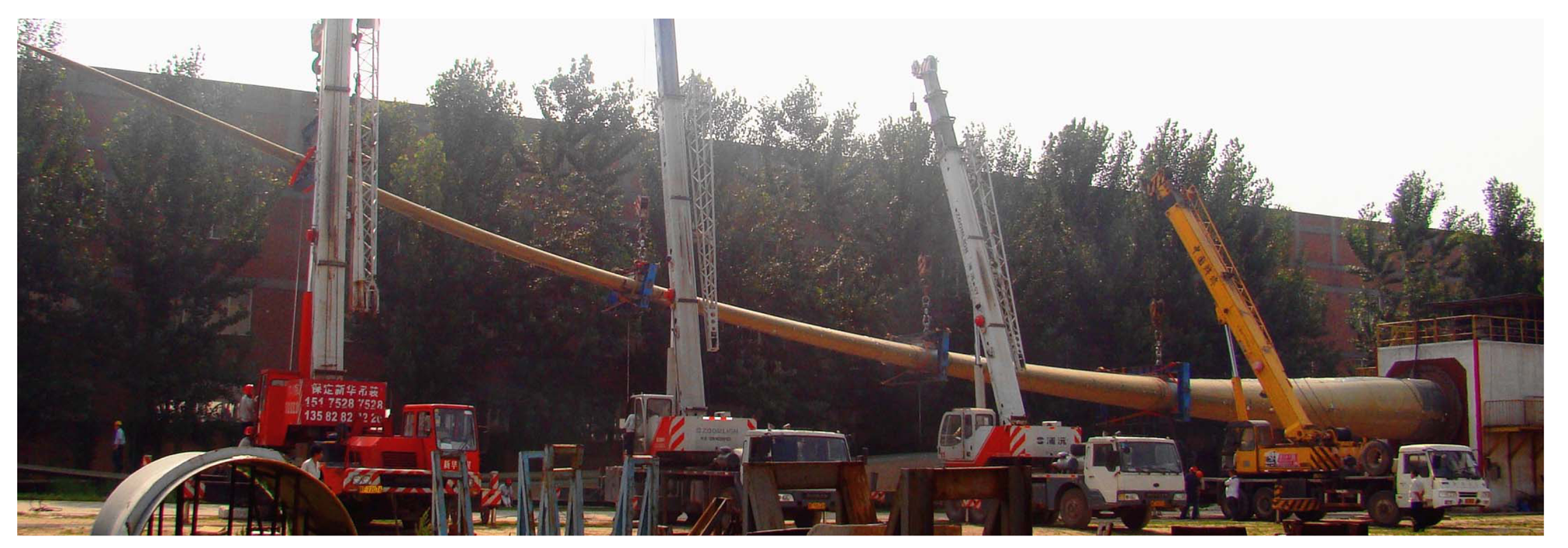
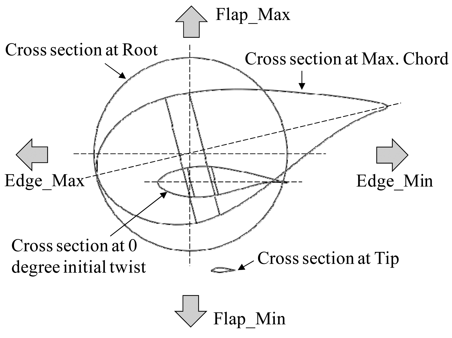
In general, two sets of static bending tests were performed on this blade, the first set was based on design loads for 2.5 MW wind turbines, and it followed the test requirements for full-scale wind turbine blades according to certification bodies. The second set was based on design loads for 3.0 MW wind turbines and it was performed with the intention to overload the blade and examine possible failure. All test cases and their sequence are shown in Table 1. Loading directions are schematically shown in Figure 3 with typical cross-sectional profiles of the blade superposed. It is noted that the test sequence of the blade was determined to comply with an order of counterclockwise rotation of the blade axis. The blade was root-fixed on a test stand as a cantilever beam and cranes applied upward pulling forces as shown in Figure 4 for the test case “F_Max_3.0”, after one test case was finished, the blade was rotated along its longitudinal axis to a prescribed position for a subsequent test case.
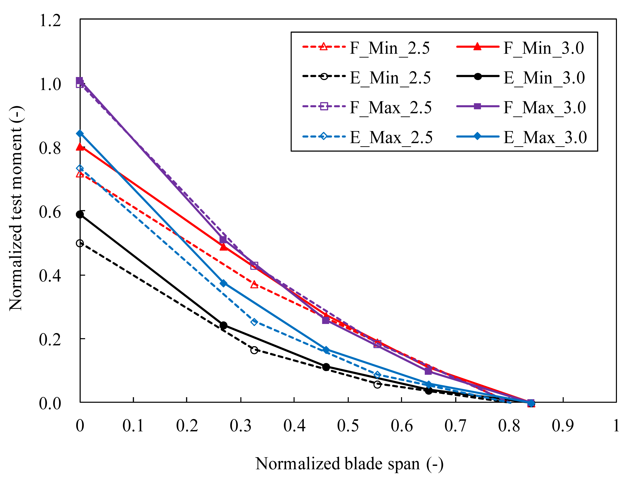
Three cranes and four cranes were used for 2.5 MW loading and 3.0 MW loading, respectively. Rubber pads with approximately 200 mm width and 15 mm thickness were installed between blade surfaces and loading saddles to reduce stress concentration at loading locations. The target test bending moments applied to the blade were normalized by the maximum root moment in the test case “F_Max_2.5” and they are shown in Figure 5. It can be seen that the target test loads of “F_Max_2.5” were basically same as those of “F_Max_3.0”. Test loads were applied in a stepwise form following a loading procedure of 0%, 40%, 60%, 80%, 100% and then an unloading procedure of 80%, 60%, 40%, 0% of the target loads in each test case. There was no communication among cranes which applied pulling force simultaneously to obtain each prescribed load level and then held for ten seconds as required by [16,17]. During the test, applied loads were recorded by load cells mounted on the cranes, deflections of the blade were measured at loading saddle locations and at blade tip using draw-wire displacement transducers, longitudinal strains were recorded by strain gauges located along the middle axis of spar caps. Average values of measurements during ten seconds were used to represent the structural response of the blade at the prescribed load levels.
2.3. Post-Mortem Observations and Discussion
After the successful completion of the 2.5 MW loading set for blade certification, the 3.0 MW loading set was followed. At 100% of the target test loads in the test case “E_Min_3.0”, trailing edge (TE) and the adjacent aft panels failed at a transition region where the cross-sectional geometry of the blade transited from a circular shape at the blade root to an airfoil shape at the maximum chord. After unloading the test case “F_Max_3.0” was followed and the blade collapsed due to a final failure at the transition region at around 90% of the target test loads. Because the target test loads of “F_Max_2.5” and “F_Max_3.0” were basically the same, the final failure load of the blade was actually 10% smaller than the load once carried by the blade.
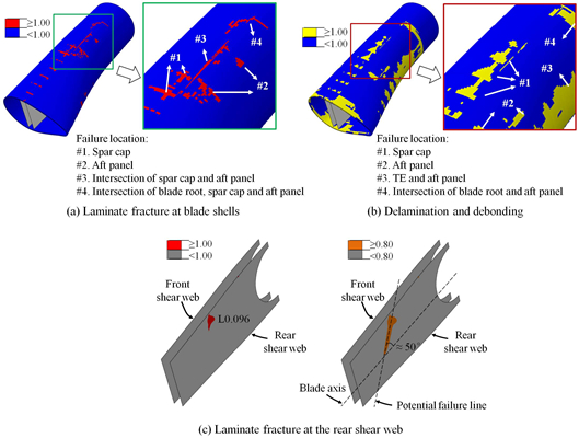
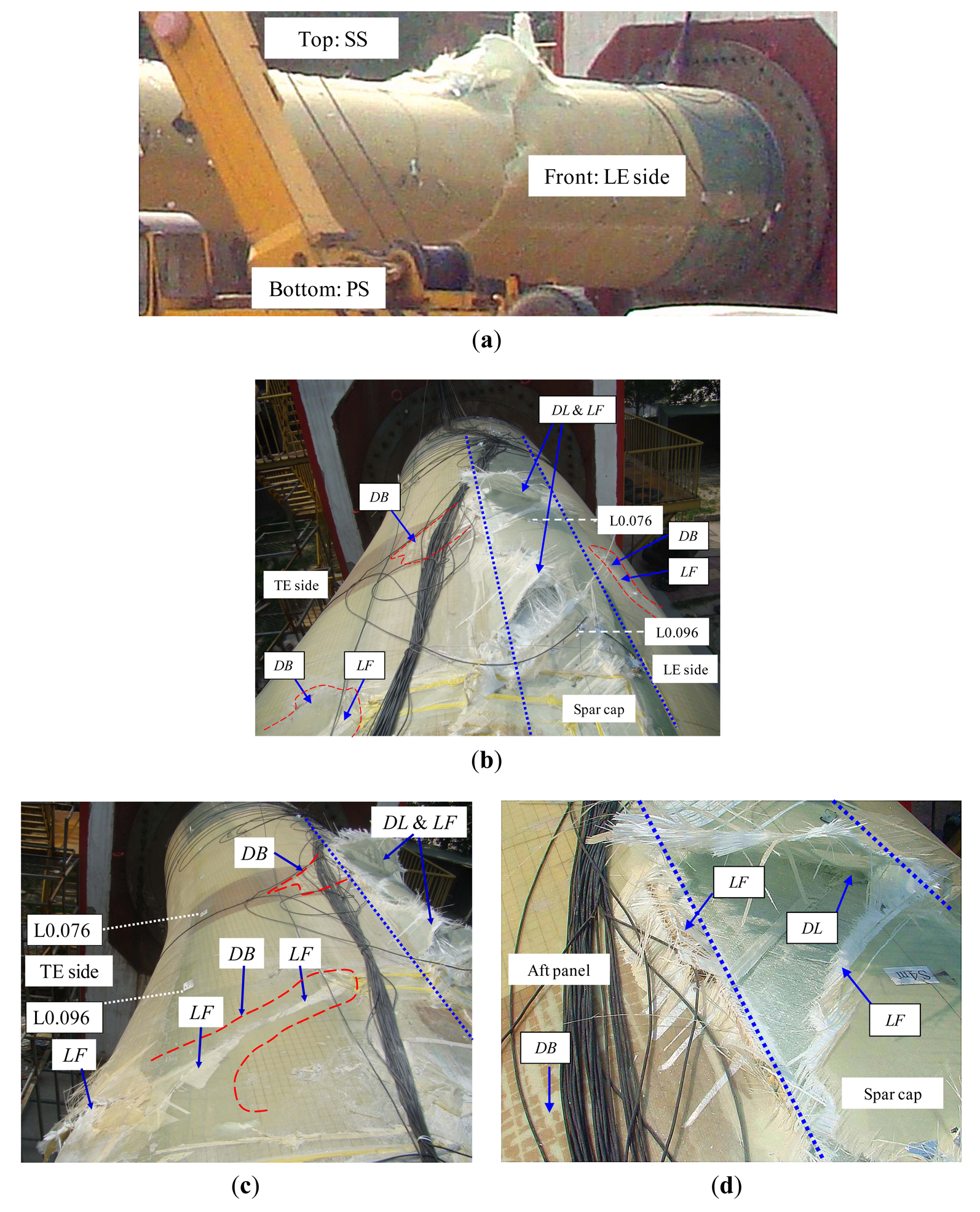
Thorough investigation was then performed on the entire blade. It was found that major failure regions were located from L0.067 to L0.105 as shown in Figure 6a. Although failed regions exhibited a complex form of failure, some typical failure modes, i.e., laminate fracture (LF), composite delamination (DL), and sandwich skin-core debonding (DB) could be identified as shown in Figure 6b,c where visually apparent debonding fronts were depicted with dashed curves, and intersections between spar cap and sandwich panels were depicted with dashed lines. A close-up of the suction side (SS) of the blade at L0.076 shows local failure characteristics in Figure 6d, and it can be seen that LF occurred at the intersection between the spar cap and aft panel, and skin laminates of spar cap were subjected to LF as well as DL.
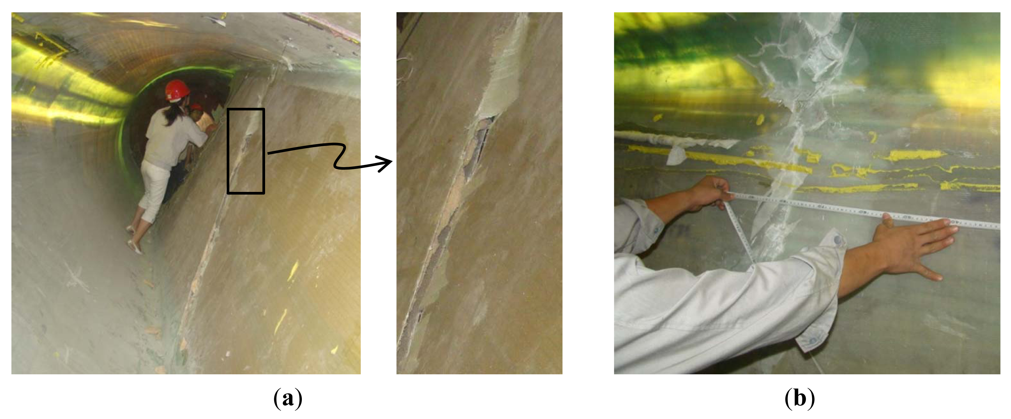
Inspection on the blade interior was also made, and it was found that the rear shear web at the location from L0.076 to L0.096 was completely failed with an approximate fracture angle of 45° to the blade axis, see Figure 7a. TE at L0.092 exhibited considerable failure with combined failure modes of LF, and DB as shown in Figure 7b.
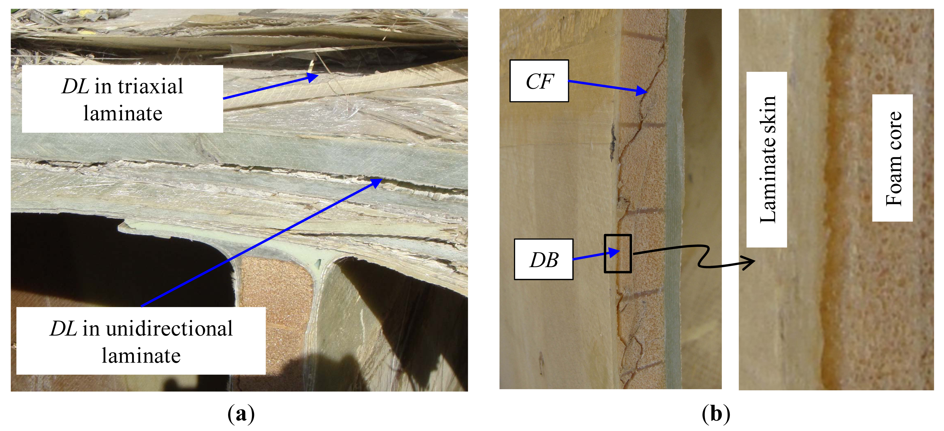
Furthermore, the blade was sectioned at L0.076 to facilitate examination on its cross-section. It was found that DL of spar cap occurred not only at triaxial laminates constituting blade skins but also at unidirectional laminates as shown in Figure 8a. Investigation on aft and LE panels revealed DB and associated core shear failure (CF) at sandwich constructions and the failure surface of DB propagated at a region roughly 1 to 2 mm underneath the interface between skin laminates and core materials as shown in Figure 8b.
From post-mortem observations, it was obvious that the transition region was pervaded by multiple failure modes. Among them DL and DB were essentially related to mechanical properties and stress states of interfaces between constituent layers and they could be categorized as interfacial (or through-thickness) failure. Another failure mode LF although commonly considered to be a form of in-plane failure was found at the intersection where geometric and material discontinuities induced interlaminar stresses inevitably affected the characteristics of LF. Because both interfacial and interlaminar stresses are closely associated with through-thickness stresses, it can be concluded that through-thickness stresses played an important role in the complex failure characteristics with multiple failure modes of the blade.
Furthermore, it is noted that spar caps with a large amount of unidirectional laminates governed the bending stiffness and the overall strength of the blade, and shear webs supported two halves of aerodynamic shells and transferred shear forces in the blade. From post-mortem observations, it can be seen that among various failure modes exhibited at the transition region delamination of unidirectional laminates in the SS spar cap and the failure of shear web were most responsible for the complete loss of the load-carrying capacity of the blade.
3. FE Modeling Method
Although post-mortem observations provided some understanding of the failure characteristics of the blade, the failure process and failure mechanisms have not been clarified yet. In order to gain more insights into the failure of the blade, a numerical model is necessary to complement the experimental study. This section, aimed at developing a FE modeling method for numerical study, first presents the considerations that have to be taken into account in the simulation and then describes material models used in the PFA techniques and a global-local approach for blade modeling. Furthermore, numerical implementation of the simulation in a commercial FE program is also presented.
3.1. Considerations in FE Modeling
Based on the failure observations from the test, it was evident that two features have to be incorporated in FE modeling in order to accurately simulate the failure process and failure characteristics of the blade. The one feature is that the FE model to be constructed should consider the effect of loading history on structural performance as the final failure load was found to be smaller than the load once carried by the blade, implying the adverse effect of loading history on its ultimate load-carrying capacity. This feature can be achieved by using well-established PFA techniques [18] which consist of two parts, i.e., failure criteria indicating occurrence of material failure and material property degradation rules representing residual properties of material once failure criteria are satisfied. Although the PFA techniques have been used in many works [19,20] to investigate failure processes of composite materials and structural components, they were rarely applied to analyze large composite blades on a structural scale. In the current study the PFA techniques were used to simulate the loading history of the blade with material failure and property degradation.
The other feature that needs to be included in the FE model are the three-dimensional stresses which enable analysis of complex failure characteristics associated with both in-plane and through-thickness stresses, and this requires solid elements to be used in the model. However, modeling and analyzing an entire blade structure using solid elements is extremely difficult due to the large differences in size scales of the component details and the entire blade. Considering that the blade failure occurred primarily at the transition region, only a local part of the blade had to be modeled and analyzed using solid elements. Although the local solid element model appeared to be a promising solution to reduce modeling difficulty, the actual loads applied to the entire blade instead of the transition region were explicitly known. In order to obtain loads sustained by the transition region, it was decided to first construct a global shell element model of the entire blade representing its load status in the test and back-calculate loads sustained by the transition region, and then these loads were applied to the local solid element model and detailed failure analysis was subsequently performed.
3.2. Material Models
3.2.1. Material Properties
Experimental results of in-plane properties from material tests are shown in Table 2. Due to commercial concerns from blade designer, all modulus and strength parameters of materials were normalized by the corresponding longitudinal properties of each material. For the local solid element model, through-thickness properties were needed to perform the analysis. However, material properties in the through-thickness (or “3”) direction were not tested in this study, so some assumptions were used to estimate these values as shown in Table 3 where the properties of unidirectional composites were regarded to be proportional to their in-plane ones, and the proportional factors were determined according to [21], in which a similar glass/epoxy unidirectional thick laminate has been systematically tested. The strength properties of two types of triaxial composites in the “3” direction were assumed to be the same as those of unidirectional composites considering that there was no fiber reinforcement aligned in this direction and strength properties were largely controlled by the matrix in composites.
In order to predict interfacial failure, i.e., DL and DB, in the solid element model, material properties of interfaces need to be known. In this study, all elastic constants and strength parameters of interfaces between two composite lamina layers were assumed to be equal to the average values of material properties of two lamina layers. As for interfaces between composite lamina and PVC foam core, material properties were assumed to be the same as PVC foam considering that the failure surface of skin-core debonding occurred in PVC foam as observed in the test.
3.2.2. Failure Criteria
Three typical failure modes, i.e., LF, DL, and DB, observed in the failed blade were considered in FE modeling. For LF, the Tsai-Wu failure criterion [22] in a three-dimensional stress field, as expressed in Equation (1), was employed in this study. The criterion is widely used to predict LF and has several advantages. It allows for interaction among stress components (analogous to the von Mises criterion for isotropic materials), it takes into account differences between tensile and compressive strength, and it is operationally simple and readily amenable to computational procedures [23]:
This failure criterion is mode-independent as it does not directly identify the nature of material damage. In order to apply appropriate material degradation rules, the nature of LF needs to be differentiated. According to Christensen [24], the term F1σ11 + F11σ112 indicates a fiber-controlled failure and it was employed to identify the fiber (or matrix)-controlled failure mode if it is larger (or smaller) than the summation of other terms in Equation (1) when failure indices exceed 1.
DL and DB were regarded as two different failure modes emphasizing their locations of occurrence, whereas they shared a similar failure feature that two constituent layers separated and the properties of their interface dominated failure behavior. Therefore, a same quadratic failure criterion based on Ye [25] as expressed in Equation (2) was employed to predict the occurrence of DL and DB:
3.2.3. Material Degradation Rules
Once failure criteria were satisfied, material properties were degraded according to certain rules representing the effect of material damage.
Some material degradation rules in the form of multiplying factors [26–28] as shown in Table 4 have been used in the failure analysis of composites, and these multiplying factors were applied to the intact material properties to obtain the degraded ones once material failure criteria were met. In the present study, the degradation rule adopted by Apalak et al. [27] was used with changing G13 value for the matrix-controlled LF from 0 to 1 regarding insignificant effect of matrix failure on transverse normal shear modulus. The value of zero was replaced by a very small value in order to avoid numerical errors in the FE analysis. The multiplying operation was only performed once at the first occurrence of the corresponding failure mode and the properties of materials hereafter remained constant, representing the irreversible nature of material damage.
3.3. FE Models
3.3.1. The Global Shell Element Model
The global shell element model was constructed in order to obtain loads sustained by the transition region by simulating a full-scale blade in the test. In this study, the general FE program Abaqus [29] which is commercially available was used. In total, about 47,300 “S4R” shell elements with a typical mesh size of 100 mm × 100 mm were used in the model. “S4R” is a 4-node, quadrilateral, stress/displacement shell element with reduced integration and a large-strain formulation. Before the final mesh size was determined, a mesh convergence study has been conducted. It was found that when the blade was modeled with typical mesh sizes of 150 mm × 150 mm, 100 mm × 100 mm, and 50 mm × 50 mm, the results of the first natural frequency between 100 mm × 100 mm mesh and 50 mm × 50 mm mesh were below 1%, and the results of the first bucking eigenvalue between two meshes were below 2%, therefore, a mesh size of 100 mm × 100 mm was deemed sufficient.
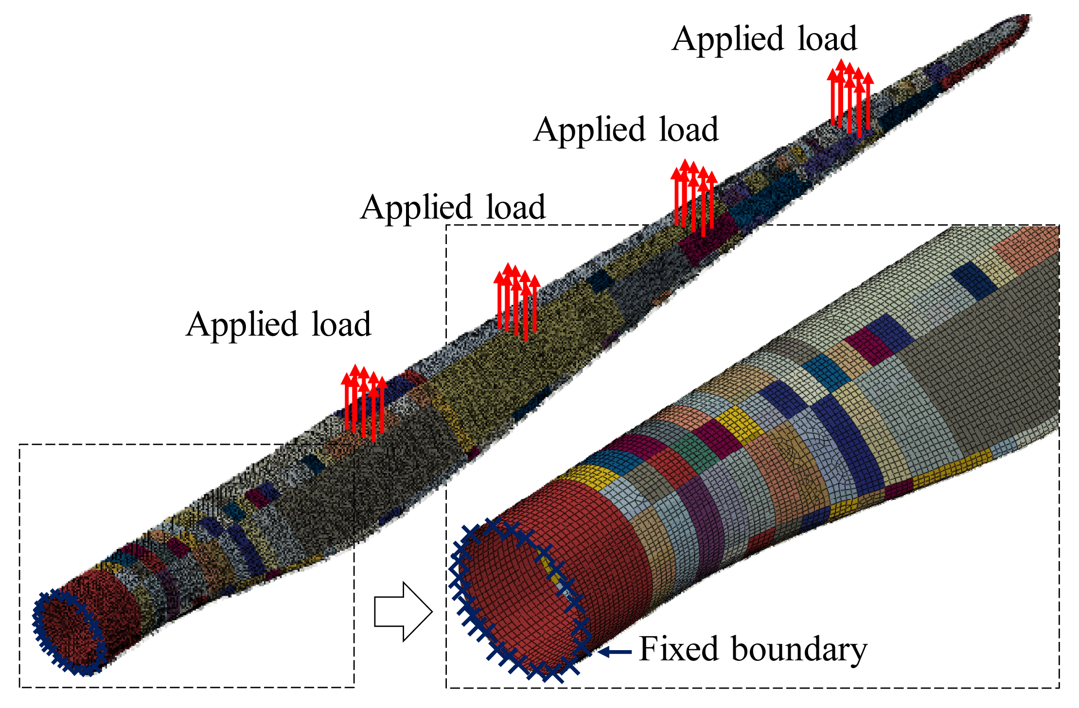
Layered orthotropic materials were applied to the blade model according to the layup scheme for blade manufacturing. A fixed boundary was applied at the blade root and point loads with resultants equal to the forces recorded from load cells were equally distributed on the surfaces where spar caps of the blade and rubber pads in the loading saddles are contacted representing actual loading setup used in the test, as shown in Figure 9. Loads were applied incrementally up to the target test loads and geometric nonlinearity was taken into account in the model to capture large deformation. Three reaction forces and three reaction moments at the blade root were extracted in every load step of each test case.
3.3.2. The Local Solid Element Model
In the present work, major blade failure of primary interest was located at the transition region approximately from L0.067 to L0.105 of the blade. Therefore, only the inboard part of the blade up to L0.134 was constructed in a local FE model. Both shell elements for shear webs and solid elements for the rest were used in the model. Nevertheless, this FE model was regarded as the local solid element model considering its different capacity to predict blade failure from the global shell element model.
There were about 25,900 solid “C3D8RC3” elements out of the total 33,000 elements used to mesh the local part. “C3D8RC3” is a 8-node, three-dimensional, linear, continuum stress/displacement element with reduced-integration. A typical mesh size was 45 mm × 45 mm for shell elements and 45 mm × 45 mm × ti for solid elements, and ti varied according to the local thickness of blade external shells. Only one solid element was used in the through-thickness direction of the blade shells. The root of the local part was fixed and multiple-point constraints (MPC) [29] were applied to a loading section at L0.134 to introduce appropriate loads through a reference point, which was positioned to have same cross-sectional coordinates as the center of the circular root section as shown in Figure 10.
Three point loads and three point moments were applied to the reference point in such a way that each reaction force and reaction moment yielded at the blade root was equal to the corresponding ones obtained from the global shell element model which was loaded according to the actual experimental setup. Layered orthotropic materials were assigned to the model. In one solid element, composite laminates were subdivided into several lamina layers with actual ply thicknesses and two types of interface layers with a negligible thickness of 0.001 mm were embedded between lamina layers, i.e., Type 1 interface layer, as well as between composite material and PVC foam core, i.e., Type 2 interface layer, as shown in Figure 11. Interface layers were employed in the solid element model in order to capture interfacial failure modes, i.e., DL and DB, in the FE analysis.
3.4. Numerical Implementation of Simulation
The PFA techniques were implemented in the solid element model to capture the complex failure characteristics observed at the transition region by incorporating user subroutines into Abaqus according to the proposed FE modeling method. The occurrences of material failure were predicted using prescribed failure criteria and material properties upon failure were degraded according to degradation rules in a three-dimensional stress field. All seven test cases were analyzed in a single numerical run following the loading history of the blade. The Riks method was adopted in order to help static equilibrium in the analysis with considerable geometric and material nonlinearities. Material failure indices larger than 1 were updated and recorded in each load increment resembling the progress of material failure in the blade.
4. Simulation Results and Discussion
This section presents results obtained from FE simulation. Two FE models used in the global-local modeling approach were assessed by comparing predicted results with experimental measurements available in the 2.5 MW loading set, and then failure process and the final failure characteristics of the transition region were predicted. Furthermore, taking advantage of the local solid element model, failure mechanisms was investigated and the Brazier effect was clarified in this section.
4.1. Model Assessment
4.1.1. Shell Model Assessment
In order to ensure that the global shell element model was able to represent the loading status of the blade in the test, numerical predictions of blade deflections and strains were compared with experimental measurements in the 2.5 MW loading set. Representatively, deflection measurements of the test case “F_Max_2.5” are shown in Figure 12a, where numerical predictions from the global shell FE model are also plotted. Longitudinal strains along spar caps at both pressure side (PS) and suction side (SS) of the blade are shown in Figure 12b.
For four test cases in the 2.5 MW loading set, longitudinal strains at SS of the blade at L0.126 are shown in Figure 12c, where arrow signs on dashed lines indicate loading and unloading paths. From these comparisons, it was found that the predicted global deflections and longitudinal strains were in satisfactory agreement with experimental measurements despite relative large difference in strains at one location as indicated with a dashed circle in Figure 12b. Therefore, the global shell element model was considered to be well constructed and can be used to calculate loads sustained by the transition region.
4.1.2. Solid Model Assessment
After applying three point loads and three point moments which back-calculated from the global shell element model to the reference point in the local solid model, the PFA was carried out to reproduce the loading history.
In order to assess the capability of the solid element model to represent the transition region of the blade in the test, the model should have been validated against experimental results, however, due to test data availability at this region, the solid element model was alternatively compared to the shell element model which has been proved to be able to predict deflections and longitudinal strains of the blade with reasonable accuracy. The test case “F_Max_2.5” was considered for the comparison representatively as shown in Figure 13 where available experimental measurements were plotted. It was found that both blade deflections and longitudinal strains obtained from the global shell element model and the local solid element model showed general agreement, despite relative large differences in strain at a few locations. Based on the comparison, it was regarded that the solid element model was loaded appropriately and was able to represent the transition region in the actual test.
4.2. Failure Prediction
4.2.1. Predicted Failure Process
Using the proposed modeling method, progressive failure process of the transition region was predicted. Due to massive results generated in the simulation, only results at the peak load of each test case were presented in this study. The locations with failure indices larger than 1 indicating material failure are shown in Figure 14.
It was found that LF was negligible until the test case “E_Min_3.0”, whereas interfacial failure in the form of DL and DB has been developed at a preceding test case “F_Max_2.5” when SS of the transition region was primarily subjected to compressive force due to applied flap-wise bending. These interfacial failure continued to progress around TE and spar cap at a subsequent test case “E_Max_2.5”. When edge-wise bending was applied in the test case “E_Min_3.0”, LF can be distinctly observed at TE and aft panels and interfacial failure spread over the transition region at various locations. Subsequently, when SS of the transition region was once again subjected to compressive force in the test case “F_Max_3.0”, LF progressed rapidly and interfacial failure was also further developed.
4.2.2. Predicted Final Failure Characteristics
The predicted final failure of the transition region was presented in a perspective view in Figure 15 for more discussion. It can be seen from Figure 15a that major regions with LF were located at SS of the blade from L0.061 to L0.086, which agreed satisfactorily with the experimental observations. Moreover, some complex failure characteristics found in the test were also well captured by the simulation, such as LF at the intersection between spar cap and aft panel. LF was also predicted to occur at intersecting regions of blade root, spar cap and aft panel although this was not visually detected in the test.
For interfacial failure as shown in Figure 15b, significant DL was found at spar cap, TE and the adjacent aft panel where similar failure characteristics were observed in the test although the scale of failure locations appeared to be overestimated. LF of the rear shear web was predicted to initiate at the top of the rear shear web at L0.096 as shown in Figure 15c. The failure region with failure indices larger than 1 was relatively small, but a contour with failure indices larger than 0.8 showed that a potential failure line originated from the initial failure location and inclined approximately 50 degree to the blade axis, which basically agreed with failure characteristics found from the post-mortem observations.
In order to examine the effect of different material degradation rules on the final failure prediction, the present material degradation rule was replaced with that used by Nagesh [26] and one new simulation was performed. The contours of the final failure obtained from two analyses were compared in Figure 16. It can be seen that failure locations predicted from the analysis with the Nagesh rule were relatively larger than those with the present one. For LF the locations with larger failure were spar cap and aft panels, and for interfacial failure, they were TE and the adjacent aft panel. Although there was a difference in the scale of the failure locations, the two analyses predicted similar results in terms of major failure locations and failure characteristics found at the transition region of the blade.
5. Failure Mechanisms
This section presented investigation on the root cause of blade failure according to experimental observations and numerical simulation. The Brazier effect, which has been argued for its role in the blade failure among several studies [6,8,10] was also examined using the numerical model.
5.1. Root Cause of the Blade Failure
Taking advantage of experimental observations and numerical simulation, the mechanisms leading to the final failure were investigated. In the 2.5 MW loading set, the transition region accumulated material damage in the form of interfacial failure, i.e., DL of unidirectional laminates in spar cap and DB in sandwich constructions. When the 3.0 MW loading set with large load amplitudes in the first two test cases, i.e., “F_Min_3.0” and “E_Min_3.0”, were applied to the blade, interfacial failure was further developed in spar cap and TE, and LF also occurred at aft panel and TE. At the test case “F_Max_3.0”, in which SS of the blade was once again subjected to compressive force in flap-wise bending, the previously developed LF continued to progress around the spar cap region with significant interfacial failure resulting in a drastic decrease of the bending stiffness and the overall strength. Meanwhile, the rear shear web started to fail further reducing its capacity to transfer shear forces. As a consequence, the blade lost its load-carrying capacity at the transition region and the final failure was witnessed. Therefore, accumulated DL of unidirectional laminates in spar cap and the following failure of shear web were considered to be the root cause of the blade failure.
5.2. The Brazier Effect
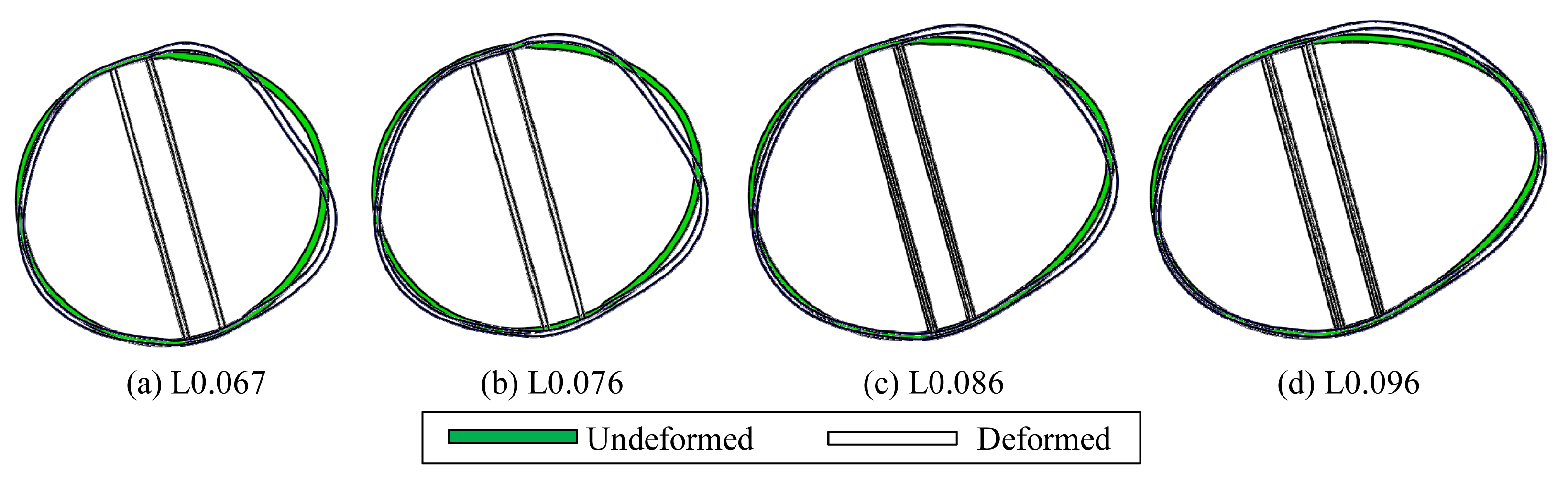
The Brazier effect was examined using the numerical model. The deformation of blade cross sections at the final failure are shown in Figure 17. The global flattening of these cross sections, which illustrates the Brazier effect, was not found in the deformed cross-sectional profiles possibly due to the constraint from shear webs between two spar caps, whereas the relative large out-of-plane deformation indicating local buckling was observed in the form of aft panel bulging outward and TE caving inward.
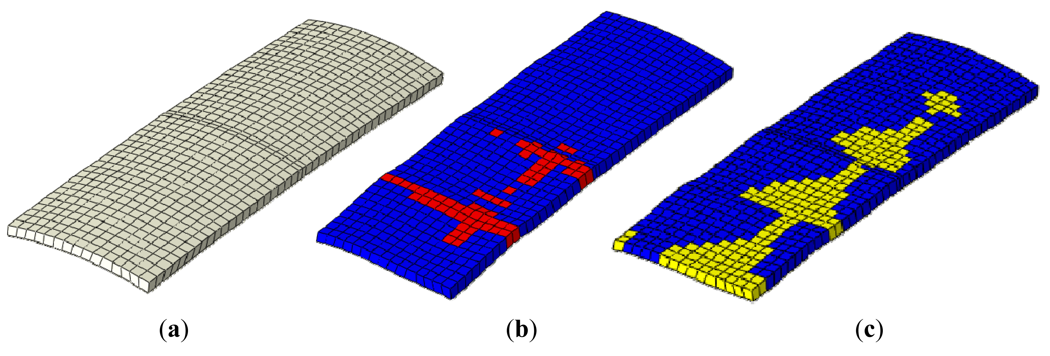
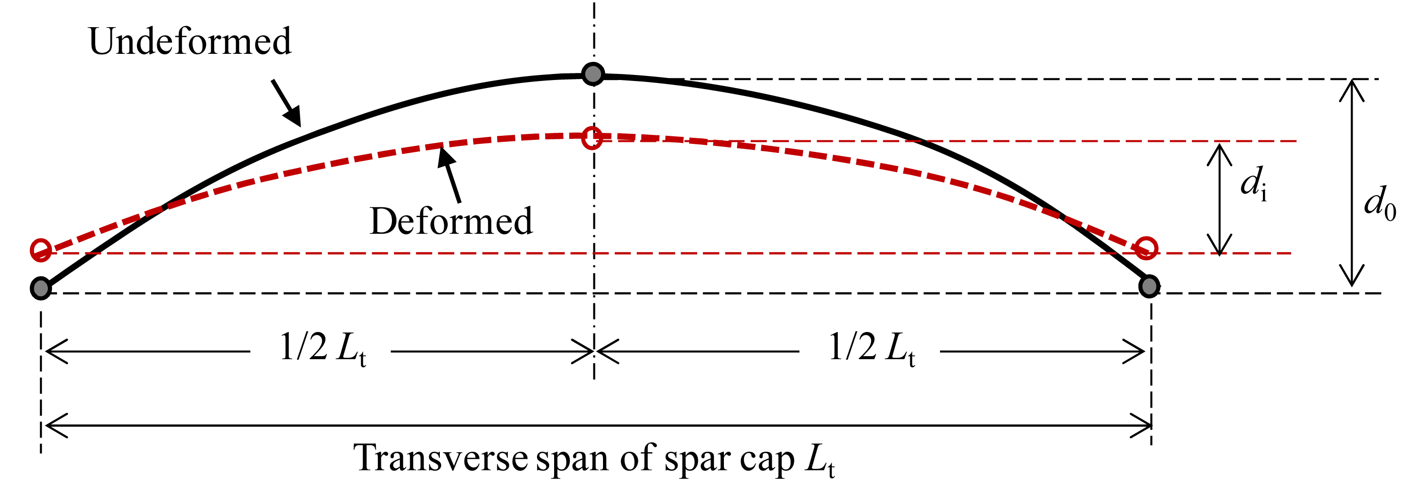
The enlarged deformation of spar cap is shown in Figure 18, and it was found that the SS spar cap, which was initially convex in the transverse direction, became flattened and exhibited buckles where interfacial failure was significant. The relative out-of-plane deformation was defined as (di − d0)/d0 × 100%, where di and d0 are the undeformed and deformed arc heights, respectively, of the spar cap at SS as shown in Figure 19.
Using this relative out-of-plane deformation, the local buckling response of spar cap was assessed quantitatively, and results at four locations of spar cap are shown in Figure 20, where initial slopes of the four curves were also plotted. It was observed that at certain load levels the curves of the relative out-of-plane deformation changed their trends and their nonlinearity became significant, and these load levels were determined as local buckling loads which had applied load fractions ranging approximately from 70% to 80%. The local buckling was expected to significantly increase out-of-plane deformation and through-thickness stresses which subsequently deteriorated DL of spar cap. Therefore, nonlinear out-of-plane deformation due to local buckling affected the failure process adversely and contributed to the blade failure.
6. Conclusions
This paper presented a thorough investigation into the failure of a 52.3 m composite wind turbine blade subjected to a series of static loads. Particular focus was placed on its complex failure characteristics observed in the test and a numerical model developed to predict failure behavior of the blade. Main conclusions can be drawn as follows: the blade failed catastrophically due to a total loss of load-carrying capacity under flap-wise bending. The final failure load was only 90% of the load once carried by the blade. Major failure was located at the transition region and characterized by multiple failure modes associated with both in-plane and more significant through-thickness stresses. Typical failure modes observed were delamination of the spar cap at the suction side, sandwich skin-core debonding, laminate fracture, and shear web failure. Among these failure modes spar cap delamination and shear web failure were indentified to be the root cause of the blade failure.
The loading history of the blade was numerically reproduced and the complex failure characteristics observed at the transition region were satisfactorily predicted in the FE simulation using the PFA techniques and a global-local modeling approach. It was found that the blade accumulated failure during its loading history. Local buckling contributed to the failure process by increasing the local out-of-plane deformation of spar cap, while the Brazier effect was not found in the transition region and it was not responsible for the failure of the blade.
This study emphasized the significance of through-thickness stresses on the failure of large composite blades. The proposed global-local modeling approach was proved to be effective to capture failure behavior of the blade while considerably reducing difficulties in modeling an entire blade.
Acknowledgments
We are grateful to several anonymous reviewers for their constructive comments that have led to significant improvement of the paper.
Conflicts of Interest
The authors declare no conflict of interest.
References
- Griffith, D.T. Technology Trends 2012. Presented at the 5th Sandia Wind Turbine Blade Workshop, Albuquerque, NM, USA, 30 May–1 June 2012.
- Ashwill, T.; Laird, D. Concepts to Facilitate Very Large Blades. Proceedings of the 45th AIAA Aerospace Sciences Meeting and Exhibit, Reno, NV, USA, 8–11 January 2007.
- Jensen, F.M.; Kling, A.; Sorensen, J.D. Change in Failure Type when Wind Turbien Baldes Scale-Up. Presented at the 5th Sandia Wind Turbine Blade Workshop, Albuquerque, NM, USA, 30 May–1 June 2012.
- Jorgensen, E.R.; Borum, K.K.; McGugan, M.; Thomsen, C.L.; Jensen, F.M.; Debel, C.P.; Sorensen, B.T. Full Scale Testing of Wind Turbine Blade to Failure—Flapwise Loading; Riso-R-1392 (EN; Riso National Laboratory: Roskilde, Denmark, 2004. [Google Scholar]
- Jensen, F.M.; Falzon, B.G.; Ankerson, J.; Stang, H. Structural testing and numerical simulation of a 34 m composite wind turbine blade. Compos. Struct. 2006, 76, 52–61. [Google Scholar]
- Jensen, F.M.; Weaver, P.M.; Cecchini, L.S.; Stang, H.; Nielsen, R.F. The Brazier effect in wind turbine blades and its influence on design. Wind Energy 2012, 15, 319–333. [Google Scholar]
- Jensen, F.M.; Puri, A.S.; Dear, J.P.; Branner, K.; Morris, A. Investigating the impact of non-linear geometrical effects on wind turbine blades—Part 1: Current status of design and test methods and future challenges in design optimization. Wind Energy 2011, 14, 239–254. [Google Scholar]
- Overgaard, L.C.T.; Lund, E.; Thomsen, O.T. Structural collapse of a wind turbine blade—Part A: Static test and equivalent single layered models. Compos. A 2010, 41, 257–270. [Google Scholar]
- Overgaard, L.C.T.; Lund, E. Structural collapse of a wind turbine blade—Part B: Progressive interlaminar failure models. Compos. A 2010, 41, 271–283. [Google Scholar]
- Yang, J.S.; Peng, C.Y.; Xiao, J.Y.; Zeng, J.C.; Xing, S.L.; Jin, J.T.; Deng, H. Structural investigation of composite wind turbine blade considering structural collapse in full-scale static tests. Compos. Struct. 2013, 97, 15–29. [Google Scholar]
- Chou, J.S.; Chiu, C.K.; Huang, I.K.; Chi, K.N. Failure analysis of wind turbine blade under critical wind loads. Engin. Fail. Anal. 2013, 27, 99–118. [Google Scholar]
- Facts, Analysis, Exposure to Industrial Wind Energy's Real Impacts. Avalilable online: http://www.windaction.org (accessed on 18 February 2014).
- Marin, J.C.; Barroso, A.; Paris, F.; Canas, J. Study of damage and repair of blades of a 300 kW wind turbine. Energy 2008, 33, 1068–1083. [Google Scholar]
- Kong, C.; Bang, J.; Sugiyama, Y. Structural investigation of composite wind turbine blade considering various load cases and fatigue life. Energy 2005, 30, 2101–2114. [Google Scholar]
- Rajadurai, J.S.; Thanigaiyarasu, G. Structural analysis, failure prediction, and cost analysis of alternative material for composite turbine blades. Mech. Adv. Mater. Struct. 2009, 16, 467–487. [Google Scholar]
- Wind Turbines-Part 1: Design Requirements, 3rd ed.; IEC standard 61400-1; International Electrotechnical Commission (IEC): London, UK, 2005.
- Guideline for the Certification of Wind Turbines; Germanischer Lloyd: Hamburg, Germany, 2010.
- Sleight, D.W. Progressive Failure Analysis Methodology for Laminated Composite Structures; NASA/TP-1999-209107; Langley Research Center: Hampton, VA, USA, 1999. [Google Scholar]
- Ridha, M.; Wang, C.H.; Chen, B.Y.; Tay, T.E. Modelling complex progressive failure in notched composite laminates with varying sizes and stacking sequences. Compos. A 2014, 58, 16–23. [Google Scholar]
- Anyfantis, K.N.; Tsouvalis, N.G. Post buckling progressive failure analysis of composite laminated stiffened panels. Appl. Compos. Mater. 2012, 19, 219–236. [Google Scholar]
- Samborsky, D.D.; Mandell, J.F.; Agastra, P. 3-D Static Elastic Constants and Strength Properties of a Glass/Epoxy Unidirectional Laminate. Available online: http://www.coe.montana.edu/composites/ (accessed on 27 November 2013).
- Tsai, S.W.; Wu, E.M. A general theory of strength for anisotropic materials. J. Compos. Mater. 1971, 5, 58–80. [Google Scholar]
- Daniel, I.M.; Ishai, O. Engineering Mechanics of Composite Materials; Oxford University Press: Oxford, UK, 1994. [Google Scholar]
- Christensen, R.M. The Theory of Material Failure; Oxford University Press: Oxford, UK, 2013. [Google Scholar]
- Ye, L. Role of matrix resin in delamination onset and growth in composite laminates. Compos. Sci. Technol. 1988, 33, 257–277. [Google Scholar]
- Nagesh. Finite-element analysis of composite pressure vessels with progressive degradation. Def. Sci. J. 2003, 53, 75–86. [Google Scholar]
- Apalak, Z.G.; Apalak, M.K.; Genc, M.S. Progressive damage modeling of an adhesively bonded composite single lap joint under flexural loads at the mesoscale level. J. Reinf. Plast. Compos. 2007, 26, 903–953. [Google Scholar]
- Tsepres, K.I.; Papanikos, P.; Kermanidis, Th. A three dimensional progressive damage model for bolted joints in composite laminates subjected to tensile loading. Fatigue Fract. Engin. Mater. Struct. 2001, 24, 663–676. [Google Scholar]
- Dassault Systemes Simulia Corp. ABAQUS/Standard User's Manual, Version 6.12; Dassault Systèmes: Providence, RI, USA, 2012. [Google Scholar]
Nomenclature
| Blade geometry | |
|---|---|
| LE | Leading edge |
| TE | Trailing edge |
| SS | Suction side |
| PS | Pressure side |
| Others | |
|---|---|
| MW | Megawatt |
| FE | Finite Element |
| PFA | Progressive Failure Analysis |
| Failure mode | |
|---|---|
| LF | Laminate fracture |
| DL | Delamination |
| DB | Sandwich skin-core debonding |
| CF | Core failure |


| Test sequence | Test case | Turbine Class | Loading direction |
|---|---|---|---|
| 1 | F_Min_2.5 | 2.5 MW | Flap_Min |
| 2 | E_Min_2.5 | Edge_Min | |
| 3 | F_Max_2.5 | Flap_Max | |
| 4 | E_Max_2.5 | Edge_Max | |
| 5 | F_Min_3.0 | 3.0 MW | Flap_Min |
| 6 | E_Min_3.0 | Edge_Min | |
| 7 | F_Max_3.0 | Flap_Max | |
| 8 * | E_Max_3.0 | Edge_Max | |
*Test case “E_Max_3.0” was not tested due to the final blade failure in “F_Max_3.0”.
| Name | Elastic constants | Strength parameters | |||||||
|---|---|---|---|---|---|---|---|---|---|
| E11 | E22 | G12 | μ12 | σ11tu | σ11cu | σ22tu | σ22cu | σ12u | |
| Unidirectional | 1 | 0.33 | 0.09 | 0.21 | 1 | −0.59 | 0.04 | −0.20 | 0.06 |
| Triaxial_7 | 1 | 0.73 | 0.51 | 0.47 | 1 | −0.94 | 0.31 | −0.86 | 0.43 |
| Triaxial_1 | 1 | 0.47 | 0.30 | 0.36 | 1 | −0.78 | 0.33 | −0.21 | 0.15 |
| Biaxial | 1 | 1.00 | 0.82 | 0.49 | 1 | −1.00 | 1.00 | −1.00 | 1.51 |
| PVC foam | 1 | 1.00 | 0.63 | 0.30 | 1 | −0.50 | 1.00 | −0.50 | 0.63 |
Where subscripts 11 and 22 mean longitudinal and transverse direction, respectively; subscript 12 means in-plane shear direction; subscripts t and c mean tensile and compressive direction, respectively; superscript u indicates ultimate strength parameters.
| Name | Elastic constants | Strength parameters | |||||||
|---|---|---|---|---|---|---|---|---|---|
| E33 | G13 | G23 | μ13 | μ23 | σ33cu | σ33tu | σ13u | σ23u | |
| Unidirectional | E22 | 1.08G12 | G12 | μ12 | 1.33μ12 | 1.03σ22cu | 0.71σ22tu | 0.97σ12u | 0.82σ12u |
| Triaxial_7 | E22 | G12 | G12 | μ12 | μ12 | = | = | = | = |
| Triaxial_1 | E22 | G12 | G12 | μ12 | μ12 | = | = | = | = |
| Biaxial | N.A. | N.A. | N.A. | N.A. | N.A. | N.A. | N.A. | N.A. | N.A. |
| PVC foam | E22 | G12 | G12 | μ12 | μ12 | σ22cu | σ22tu | σ12u | σ12u |
Note: “=” means that the value is the same as that for unidirectional composite; “N.A.” means “not applicable”, it is because biaxial materials are used in shear webs, which are modeled with shell elements, and their through-thickness properties are not needed in the FE model.
| Failure mode | Model | E11 | E22 | E33 | G12 | G13 | G23 | μ12 | μ13 | μ23 |
|---|---|---|---|---|---|---|---|---|---|---|
| LF (Fiber-controlled) | Nagesh [26] | 0.1 | 0.1 | 0.1 | 0.1 | 0.1 | 0.1 | 0 | 1 | 1 |
| Z.G. Apalak et al. [27] | 0 | 0 | 0 | 0 | 0 | 0 | 0 | 0 | 0 | |
| K.I. Tserpes et al. [28] | 0 | 0 | 0 | 0 | 0 | 0 | 0 | 0 | 0 | |
| Present | 0 | 0 | 0 | 0 | 0 | 0 | 0 | 0 | 0 | |
| LF (Matrix-controlled) | Nagesh [26] | 1 | 0.1 | 0.1 | 1 | 1 | 0.1 | 0 | 0 | 1 |
| Z.G. Apalak et al. [27] | 1 | 0 | 0 | 1 | 0 | 0 | 0 | 0 | 1 | |
| K.I. Tserpes et al. [28] | 1 | 0 | 1 | 1 | 1 | 1 | 0 | 1 | 1 | |
| Present | 1 | 0 | 0 | 1 | 1 | 0 | 0 | 0 | 1 | |
| DL | Nagesh [26] | 1 | 0.1 | 0.1 | 1 | 1 | 0.1 | 0 | 0 | 1 |
| Z.G. Apalak et al. [27] | 1 | 1 | 0 | 1 | 0 | 0 | 1 | 0 | 0 | |
| K.I. Tserpes et al. [28] | 1 | 1 | 0 | 1 | 0 | 0 | 1 | 0 | 0 | |
| DL&DB | Present | 1 | 1 | 0 | 1 | 0 | 0 | 1 | 0 | 0 |
© 2014 by the authors; licensee MDPI, Basel, Switzerland. This article is an open access article distributed under the terms and conditions of the Creative Commons Attribution license ( http://creativecommons.org/licenses/by/3.0/).
Share and Cite
Chen, X.; Zhao, W.; Zhao, X.L.; Xu, J.Z. Failure Test and Finite Element Simulation of a Large Wind Turbine Composite Blade under Static Loading. Energies 2014, 7, 2274-2297. https://doi.org/10.3390/en7042274
Chen X, Zhao W, Zhao XL, Xu JZ. Failure Test and Finite Element Simulation of a Large Wind Turbine Composite Blade under Static Loading. Energies. 2014; 7(4):2274-2297. https://doi.org/10.3390/en7042274
Chicago/Turabian StyleChen, Xiao, Wei Zhao, Xiao Lu Zhao, and Jian Zhong Xu. 2014. "Failure Test and Finite Element Simulation of a Large Wind Turbine Composite Blade under Static Loading" Energies 7, no. 4: 2274-2297. https://doi.org/10.3390/en7042274