Modeling and Parameterization of Fuel Economy in Heavy Duty Vehicles (HDVs)

Abstract

The present paper suggests fuel consumption modeling for HDVs based on the code from the Japanese Ministry of the Environment. Two interpolation models (inversed distance weighted (IDW) and Hermite) and three types of fuel efficiency maps (coarse, medium, and dense) were adopted to determine the most appropriate combination for further studies. Finally, sensitivity analysis studies were conducted to determine which parameters greatly impact the fuel efficiency prediction results for HDVs. While vitiating each parameter at specific percentages (±1%, ±3%, ±5%, ±10%), the change rate of the fuel efficiency results was analyzed, and the main factors affecting fuel efficiency were summarized. As a result, the Japanese transformation algorithm program showed good agreement with slightly increased prediction accuracy for the fuel efficiency test results when applying the Hermite interpolation method compared to IDW interpolation. The prediction accuracy of fuel efficiency remained unchanged regardless of the chosen fuel efficiency map data density. According to the sensitivity analysis study, three parameters (fuel consumption map data, driving force, and gross vehicle weight) have the greatest impact on fuel efficiency (±5% to ±10% changes).

1. Introduction

Studies of Medium and Heavy Duty Vehicles (MHDVs) are being emphasized due to the reinforcement of greenhouse emissions regulation and awareness of the resource depletion crisis. The total fuel consumption portion of MHDVs in the US is about 26%, and other countries also have high fuel consumption in the MHDV sector [1]. Therefore, many government agencies are considering this issue to control environmental problems and promote energy conservation in the MHDV sector. With existing emission regulations for light-duty vehicles, new regulations for MHDVs have been enacted by some governments. Japan first declared the fuel consumption test method standards and regulations for Heavy Duty Vehicles (HDVs) in 2006 and the US also enacted the regulations for MHDVs in 2010 [2,3,4].

Those issues have been continuously considered and addressed worldwide, yet most countries do not publicize the specific regulations. In order to establish regulation criteria, many studies are need to reflect the circumstances of their each country, but there are many variables to consider. Environmental factors such as seasonal, topographical and driving style differences can largely impact on the fuel economy and exhaust characteristics of vehicles. Even for the same vehicle model, MHDV specification can be divided into hundreds to thousands of models due to the manufacturing process. MHDVs are commonly manufactured differently depending on the customer’s need, whereas light duty vehicles generally have a similar purpose and are almost uniformly manufactured to the same general specifications. Some specifications (such as vehicle mass, power, size) are reported to have a greater impact on vehicle performance. Therefore, all of these parameters should be reflected in vehicle tests [5,6]. Also, the importance of implementing a realistic test driving mode (vehicle velocity profile according to time) according to each country’s infrastructure is being emphasized. For example, Japan and South Korea have high population densities, and the portion of highways is less than in the US, so vehicular lane changes (gear shifting) occur more frequently, which can reduce fuel economy [7]. These considerations are essential to providing customers with the exact fuel economy and vehicle performance of their own vehicles and to implementing advanced regulations that are adequate for domestic circumstances.

However, such testing that considers all these variables is expense and time consuming. One of the problems in using a chassis dynamometer for HDVs is the low penetration rate due to the high price. Therefore, the test method cannot match the rapid change of worldwide fuel economy and emissions regulations for MHDVs. Thus, simulation methods are suggested in parallel with existing test methods to reduce the testing burden on government agencies (US, Japan, China and EU) and manufacturing companies [5,8,9]. These approaches are currently being used to support the theoretical basis for future regulations, reduce unnecessary experimental conditions and perform a diverse parametric study in the short term.

Currently, diverse forms of vehicle simulation tools have been developed and provided in many research fields. The AVL Company sells the commercial tool called CRUISE, which offers diverse forms of graphic user interfaces and examples of a basic vehicle modeling module (conventional, hybrid, electric, and HDV). The structure of this program can also reflect the experimental data in the calculation process and newly developed vehicle component model [10]. In the US, the Environmental Protection Agency (EPA) and the National Highway Traffic Safety Administration (NHTSA) jointly proposed the Greenhouse Emission Model (GEM, US) program to improve the emission characteristics and fuel efficiency of MHDVs [11]. This program divides MHDVs vehicles into seven classes (2b to 8) on the basis of gross vehicle weight (GVW) and provides default specifications and fuel economy maps for each class. Therefore, it is useful for a user who wants approximate predictions for specific vehicles in a short time. Meanwhile, the transformation algorithm program code (Ministry of the Environment, Japan) has been released in in-house code forms (C++ and FORTRAN90). This program performs calculations based on vehicle specifications and driving mode (vehicle speed according to time) data and predicts the optimum gear position, engine speed, and engine torque according to the time domain. There is a disadvantage in that the post-processing algorithm is not contained in this program, so users must make their own post-processing algorithm, and the fuel consumption map data should be added as input data to predict the final fuel efficiency of the subject MHDV vehicle [12]. However, the main structure of this program code is simpler than that of other programs, so it is easier to modify of existing models or add new vehicle models into the program. Also, it is reported that overall prediction results are highly accurate. According to Sato et al. [13], the error in the simulation compared to the actual measurement is limited to about 0.4% regardless of the type of HDV. The EU also recognizes the advantage of using simulation methods to more efficiently evaluate vehicle performance than test-based approach, including the premise that vehicle tests should also be performed to validate the predicted results [14]. The European Automobile Manufacturers Association (ACEA) is officially developing a simulation tool that will be available to government agencies, customers, and manufacturers.

In China, comparative analysis of the merits and demerits of existing test methods led to the adoption of simulation modeling as one of the test methods for HDV standards. The program developed by the China Automotive Technology and Research Center (CATARC) offers two kinds of calculation methods: one is the basic type which reflects fuel consumption data obtained from the chassis dynamometer test, and the other is the variant type which reflects fuel consumption data based on computational simulation [15].

This study adopts the transformation algorithm program proposed by the Japanese Ministry of the Environment to predict the fuel efficiency of HDVs. The pre-processor is slightly modified to reflect the additional input data, and a post-processor is added to predict the final fuel efficiency results. The main procedure of this study is divided into two parts. First, comparative analysis of the simulation result data is conducted based on different interpolation methods (inversed distance weighted (IDW) and Hermite), and one of these two methods is selected to increase the prediction accuracy of the final HDV fuel efficiency. Also, the impact of the density of the fuel efficiency map data on prediction accuracy was studied. It is expected that this approach will show the optimum fuel efficiency map data type. Sensitivity analysis of factors that impact the prediction results is conducted by changing the values of the major factors at particular percentage intervals. Through this study, we aim to classify the main factors that affect the fuel efficiency of HDVs. A more quantitative prediction of HDV fuel efficiency is expected by changing the HDV’s basic specifications and reducing research costs by eliminating needless test conditions.

2. Model Architecture

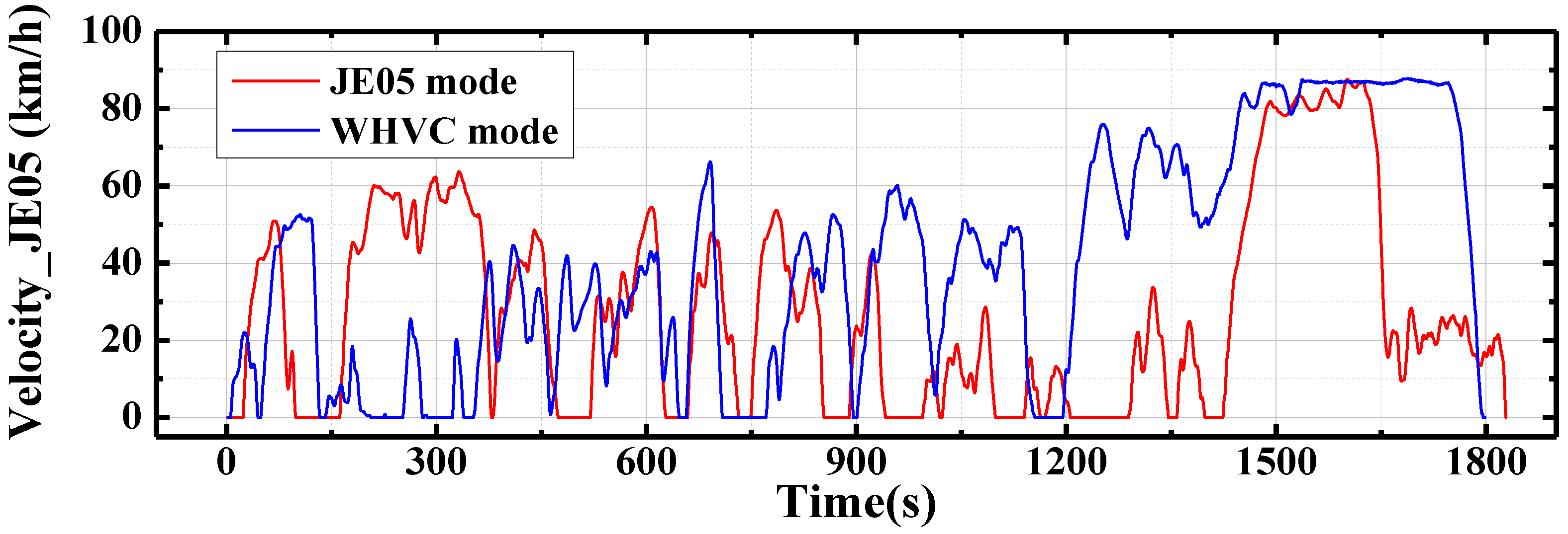
The vehicle model consists of three main parts: pre-processor, main processor, and post processor. The transformation algorithm program does not contain the post processor, so users add this part to calculate the final fuel efficiency of the HDV. The pre-processor reads the input data needed in calculations, such as maximum torque data (Figure 1), vehicle specifications, fuel consumption map and driving mode (Figure 2).

Figure 1. Sample of maximum torque date [12].

Figure 1. Sample of maximum torque date [12].

Figure 2. Driving mode data (JE05 & WHVC mode).

Figure 2. Driving mode data (JE05 & WHVC mode).

Also, the pre-processor conducts some calculations to acquire additional input data such as engine and tire rotational weight, air resistance coefficient (Equation (1)), and rolling resistance coefficient (Equation (2)) based on vehicle dynamic theories. In the case of a bus, the correction factor (fixed constant value, 0.680) is multiplied by the air resistance coefficient:

$${\text{μ}}_{\text{a}}\text{A }=0.00299\times B\times H-0.000832$$

(1)

$${\text{μ}}_{\text{r}}=0.0513+\left(17.6/W\right)$$

(2)

where μ_a is the air drag coefficient; A is the frontal area (unit: m²); B is the width of the HDV (unit: m); H is the height of the HDV (unit: m); μ_r is the rolling resistance coefficient; and W is the test vehicle weight (unit: kg). The test vehicle weight is defined as the sum of the empty vehicle weight and half of the HDV’s load capacity. The gross weight of the test HDV is defined as shown in following Equations (3) and (4) [16]:

$$\text{Gross weight of truck and tractor }=W_{\text{c}}+L_{\text{Max}}/2+W_{\text{driver}}$$

(3)

$$\text{Gross weight of bus }=W_{\text{c}}+R_{\text{Max}}/2\times W_{\text{driver}}$$

(4)

where W_c is the curb weight of HDV (unit: kg); L_Max is the maximum load (unit: kg); R_Max is the riding capacity (unit: number of passengers); and W_driver is the body weight of an average person (unit: kg, fixed as a constant value of 55 kg).

Based on these input data, the main processor performs several calculations. This part defines the vehicle operating conditions appropriate for various operating statuses. In addition, some considerations are made for vehicle operating status, such as reacceleration and deceleration. One of the important calculation procedures in the main process is to calculate the optimum engine speed and torque at each driving time. The Japanese transformation algorithm program [12] basically contains a sub-program that predicts the engine state based on torque margin. The torque margin is an important factor that determines the available torque normally transferred to the drive shaft system, as defined in Equation (5):

$$T_{\text{margin}}=T_{\max }/T_{\text{driving}}$$

(5)

where T_margin is the torque margin; T_max is the maximum engine torque (unit: Nm); and T_driving is the torque needed to drive the vehicle (unit: Nm). If the torque margin is less than 1 at a specific driving point, then the driving condition is unstable, and the gear position should be changed to increase the engine torque. In order to calculate the torque margin, the total driving resistance is defined as the sum of rolling resistance, air drag resistance, and acceleration force needed for the vehicle to move forward (Equation (6)). The maximum engine torque data is acquired as an input data in the form shown in Figure 1, and driving torque is derived by Equation (7) [16]:

$$R={\text{μ}}_{\text{r}}W+\frac{s}{100}W+{\text{μ}}_{a}A{V}^2+\left(W+\Delta W_1+\Delta W_2\right)\frac{a}{g}$$

(6)

$$T_{\text{driving}}=\frac{r\cdot {\eta }_{\text{tg}}\cdot {\eta }_{\text{fg}}}{i_{\text{tg}}\cdot i_{\text{fg}}}\cdot R$$

(7)

where R is the driving resistance (unit: N); s is the longitudinal grade (unit: %); V is the vehicle speed (unit: km/h); ΔW₁ and ΔW₂ are the rotational weight of the engine and flywheel and other components (unit: N) respectively; a is the vehicle acceleration (unit: m/s²); g is the acceleration by gravity; r is the tire dynamic load radius (unit: m); η_tg and η_fg are the mechanical transmission efficiencies of the transmission gear and final reduction gear; and i_tg and i_fg are the transmission and final reduction gear ratio. Based on the calculation results for the torque margin and other engine state data, the Japanese transformation algorithm program defines the engine operation conditions by six cases, as shown in Table 1.

Table 1. Definitions of engine operating states in simulation program.

Case	Engine operating state
1	Engine speed and torque are in range
2	Lack of engine torque, engine speed is in range
3	Engine over-revolution, engine torque is in range
4	Lack of engine speed (occurs when vehicle has to re-accelerate)
5	Clutch release
6	Vehicle start mode, gear position = 1st or 2nd

Table 1. Definitions of engine operating states in simulation program.

Case	Engine operating state
1	Engine speed and torque are in range
2	Lack of engine torque, engine speed is in range
3	Engine over-revolution, engine torque is in range
4	Lack of engine speed (occurs when vehicle has to re-accelerate)
5	Clutch release
6	Vehicle start mode, gear position = 1st or 2nd

In this program, the sub-programs related to gear shifting aim to change gear positions changes at each time step. Except for case 1 (engine speed and torque are in range), the program changes the gear position in order to determine the optimum engine operating conditions (engine speed and torque and final gear position). Also, the minimum gear holding time (3 s) is fixed to prevent the frequent gear position changes. For example, in the case of a vehicle that needs more engine torque in order to accelerate, the program first shifts the gear position down one step. If the engine speed and torque are in range as a result of downshifting one step, the program verifies that the changed gear position can be maintained for 3 s. The calculation procedure can continue to the next time step if the new gear position meets all the requirements. However, the program shifts another gear to find the optimum gear position if the new gear position does not meets the requirements. The gear shifting is set to not exceed more than four step in single gear shifting time. From all these calculation procedures, we can predict the optimal gear position, engine speed, and torque according to driving mode.

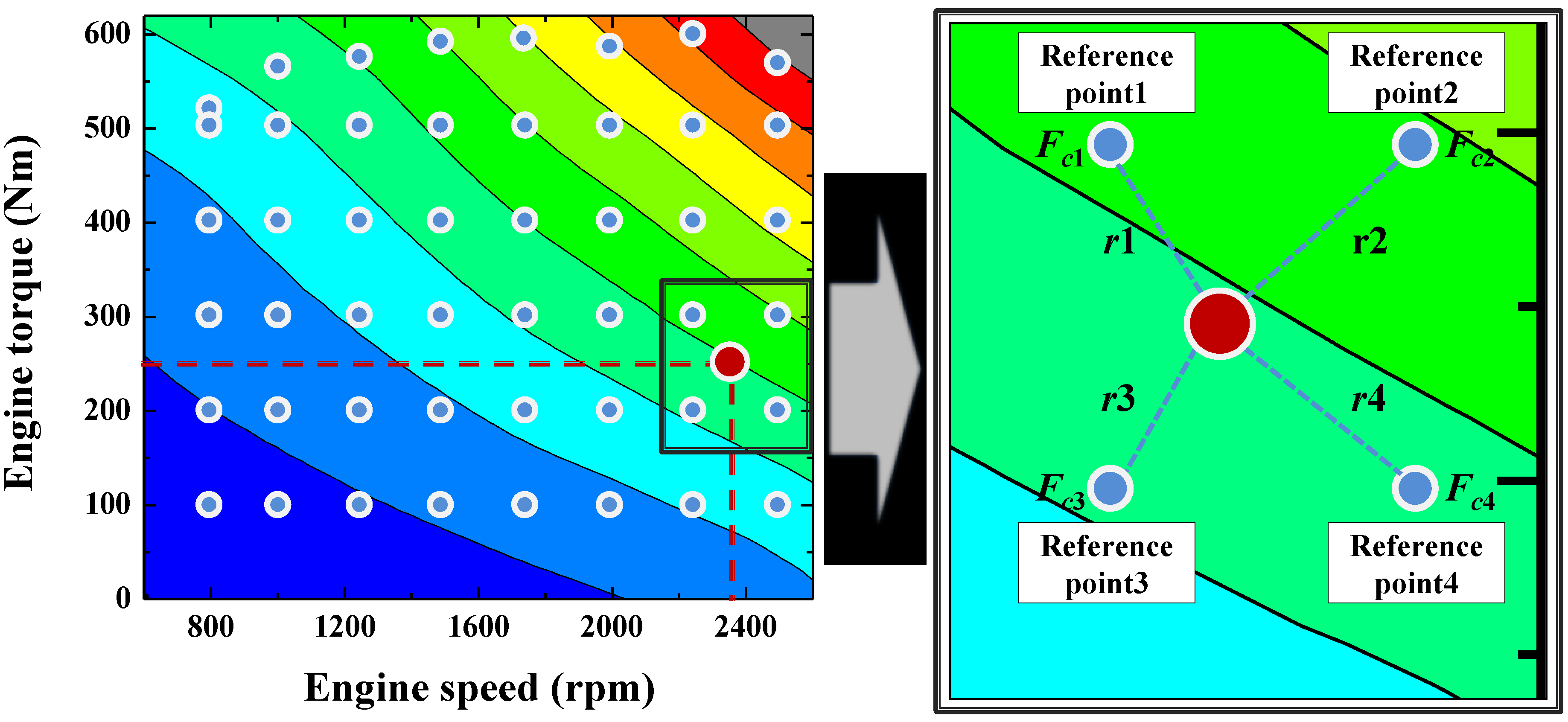
The two types of interpolation method (IDW and Hermite) were adopted in this study. In the case of the IDW interpolation method, the program was set to select the four reference points near the specific revolution-torque combinations, as seen in Figure 3, and the fuel consumption rates at each time step were defined as in Equation (8):

$$F_c=\frac{F_{c1}/r_1+F_{c2}/r_2+F_{c3}/r_3+F_{c4}/r_4}{1/r_1+1/r_2+1/r_3+1/r_4}$$

(8)

where F_c1–F_c4 is the fuel consumption rate at each reference point; r₁–r₄ is the two-dimensional distance between reference points and the specific revolution-torque point; and F_c is the fuel consumption rate at the specific revolution-torque point. In the calculation process, the gradient information was not considered, and the fuel consumption rate was defined in proportion to the distance.

Figure 3. Definition of the fuel consumption rate by applying the IDW interpolation method.

Figure 3. Definition of the fuel consumption rate by applying the IDW interpolation method.

Meanwhile, the piecewise cubic Hermite interpolation method [17] generates the cubic equations on each interval. Thus, it has an advantage that considering gradient data into the calculation process compared to IDW method. The fuel consumption rates at each time step were defined as in Equations (9)–(13):

$$F_c(x)=c_0+c_1\left(x-x_{i-1}\right)+c_2{\left(x-x_{i-1}\right)}^2+c_3{\left(x-x_{i-1}\right)}^3$$

(9)

$$c_0=F_c\left(x_{i-1}\right)$$

(10)

$$c_1=F_c^{\prime }\left(x_{i-1}\right)$$

(11)

$$c_2=3\left(F_c\left(x_i\right)-F_c\left(x_{i-1}\right)\right)/h^2-\left({F^{\prime }}_c\left(x_i\right)+2F_c^{\prime }\left(x_{i-1}\right)\right)/h$$

(12)

$$c_3=\left(F_c^{\prime }\left(x_i\right)+F_c^{\prime }\left(x_{i-1}\right)\right)/h^2-2\left(F_c\left(x_i\right)-F_c\left(x_{i-1}\right)\right)/h^3$$

(13)

where x is the target point which is test vehicle operating condition in specific time; x_i−1 and x_i is the reference points near the target point; h is the interval length. In order to get a c₀–c₃ constant values; F_c(x_i) and F_c(x_i−1) is the fuel consumption rate of the reference points; F_c′(x_i) and F_c′(x_i−1) is the derivative information. The F_c(x_i) and F_c(x_i−1) are known value whereas F_c′(x_i) and F_c′(x_i−1) are unknown value because the fuel efficiency map data basically not containing derivative information. To solve this problem, gradient algorithm is added in program. This algorithm set to calculate the gradient at each test point based on nearby reference points in this program.

3. Experimental Approach

In this study, the HDV chassis dynamometer (AVL Zollner, Graz, Austria) test was performed to validate the accuracy of the Japanese transformation algorithm program. The driver and vehicle speed monitoring system are applied to drive the HDV on the dynamometer in JE05 and WHVC mode. The chassis dynamometer system is a Motor In the Middle (MIM) type in which the fuel measuring system is connected to a test vehicle to determine a fuel consumption rate at each time step. The detailed specifications of the chassis dynamometer and techniques of emission analysis are shown in Table 2 and Table 3. The specifications of two test vehicles which are adopted to conduct the urban cycle mode test are shown on Table 4.

Table 2. Specifications of HDV chassis dynamometer.

Major items	Specification
Roller Diameter	72" (1,828.8 mm)
Roller Width	2,800 mm and 900 mm
DYNO Motor Power/Absorbing (continuous)	450 kW
Max test speed	160 km/h
Base Inertia	7,038 kg
Inertia simulation range	3,500–30,000 kg
Pul down system with load-cell	Max Force: 10,000 kg
Max permissible axle load	20,000 kg
Restraint chain system	Max tractive force 40,000 N
Tolerance of speed value and Actual Force	0–1 km/h (0.1%), 2–160 km (0.01%)/0.1%

Table 2. Specifications of HDV chassis dynamometer.

Major items	Specification
Roller Diameter	72" (1,828.8 mm)
Roller Width	2,800 mm and 900 mm
DYNO Motor Power/Absorbing (continuous)	450 kW
Max test speed	160 km/h
Base Inertia	7,038 kg
Inertia simulation range	3,500–30,000 kg
Pul down system with load-cell	Max Force: 10,000 kg
Max permissible axle load	20,000 kg
Restraint chain system	Max tractive force 40,000 N
Tolerance of speed value and Actual Force	0–1 km/h (0.1%), 2–160 km (0.01%)/0.1%

Table 3. Specifications of emission measurement system.

Gas	Technique	Typical Range
CO2	Non-dispersive infra-red	0–0.5 … 20 vol%
THC	Heated flame ionization detector	0–10 … 5,000 ppm or more
NO/NOX	Chemiluminescence detector	0–10 … 5,000 ppm or more

Table 3. Specifications of emission measurement system.

Gas	Technique	Typical Range
CO2	Non-dispersive infra-red	0–0.5 … 20 vol%
THC	Heated flame ionization detector	0–10 … 5,000 ppm or more
NO/NOX	Chemiluminescence detector	0–10 … 5,000 ppm or more

Table 4. Specifications of HDVs implemented in the fuel efficiency test.

Type	Vehicle specifications		Gear ratio
Vehicle A	Vehicle weight at test (kg)	8,215	1	6.967
	idling speed (rpm)	600	2	4.247
	Max. power (ps)	220	3	2.454
	Max. torque (kgm)	65	4	1.471
	Dimensions (m)	Width: 3.250, Height: 2.490	5	1.000
Vehicle B	Vehicle weight at test (kg)	14,775	1	3.428
	idling speed (rpm)	600	2	2.007
	Max. power (ps)	300/2,200 rpm	3	1.416
	Max. torque (kgm)	115/1,200 rpm	4	1.000
	Dimensions (m)	Width: 3.250, Height: 2.490	5	0.830

Table 4. Specifications of HDVs implemented in the fuel efficiency test.

Type	Vehicle specifications		Gear ratio
Vehicle A	Vehicle weight at test (kg)	8,215	1	6.967
	idling speed (rpm)	600	2	4.247
	Max. power (ps)	220	3	2.454
	Max. torque (kgm)	65	4	1.471
	Dimensions (m)	Width: 3.250, Height: 2.490	5	1.000
Vehicle B	Vehicle weight at test (kg)	14,775	1	3.428
	idling speed (rpm)	600	2	2.007
	Max. power (ps)	300/2,200 rpm	3	1.416
	Max. torque (kgm)	115/1,200 rpm	4	1.000
	Dimensions (m)	Width: 3.250, Height: 2.490	5	0.830

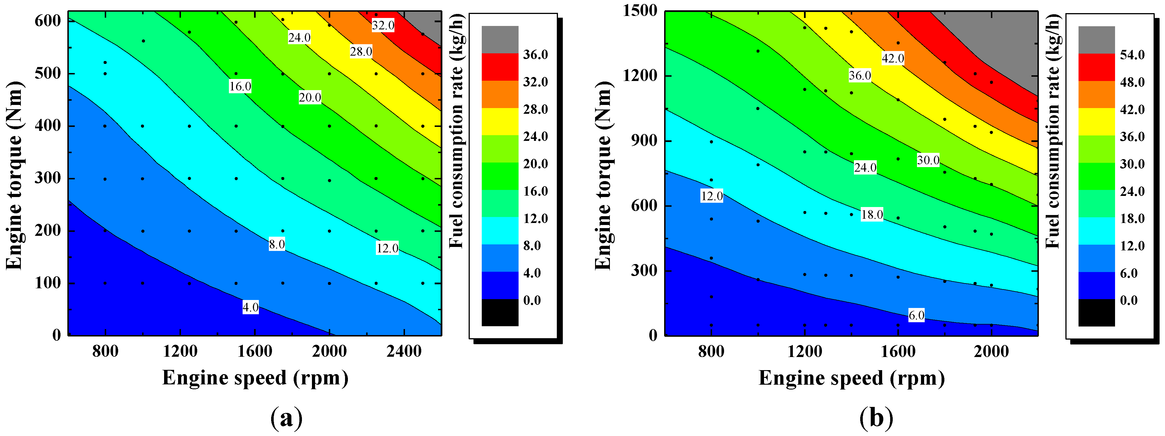
The gross weight is defined as the sum of the empty vehicle weight and half the riding rate of the test HDV’s limit capacity as noted previously. The gross weight of vehicle1 is smaller than that of vehicle2; it is expected that the test and simulation results of the two vehicles will show different trends. In order to predict the fuel efficiency of test HDVs, the fuel consumption map is the most important input data. The Committee for Natural Resource and Energy (CNRE, Tokyo, Japan) proposes that the fuel efficiency map should be created as a combination of the engine revolution (at least six points in the range between the lowest and highest revolutions) and torque (at least five points in the range between zero and full load torque) [16]. The implementation of the interpolation method is also proposed if the fuel consumption rate data does not exist at the given revolution-torque combinations. Based on these standard proposals, engine mode tests were conducted as shown in Figure 4, and two fuel consumption maps were adopted in a simulation study, as shown in Figure 5. The fuel consumption rate shows some characteristics that proportional to engine torque and inverse proportional to engine speed. These data were acquired from a report by the Korea Energy Management Cooperation (KEMC, Sungnam, Korea) [18].

Figure 4. Engine test points.

Figure 4. Engine test points.

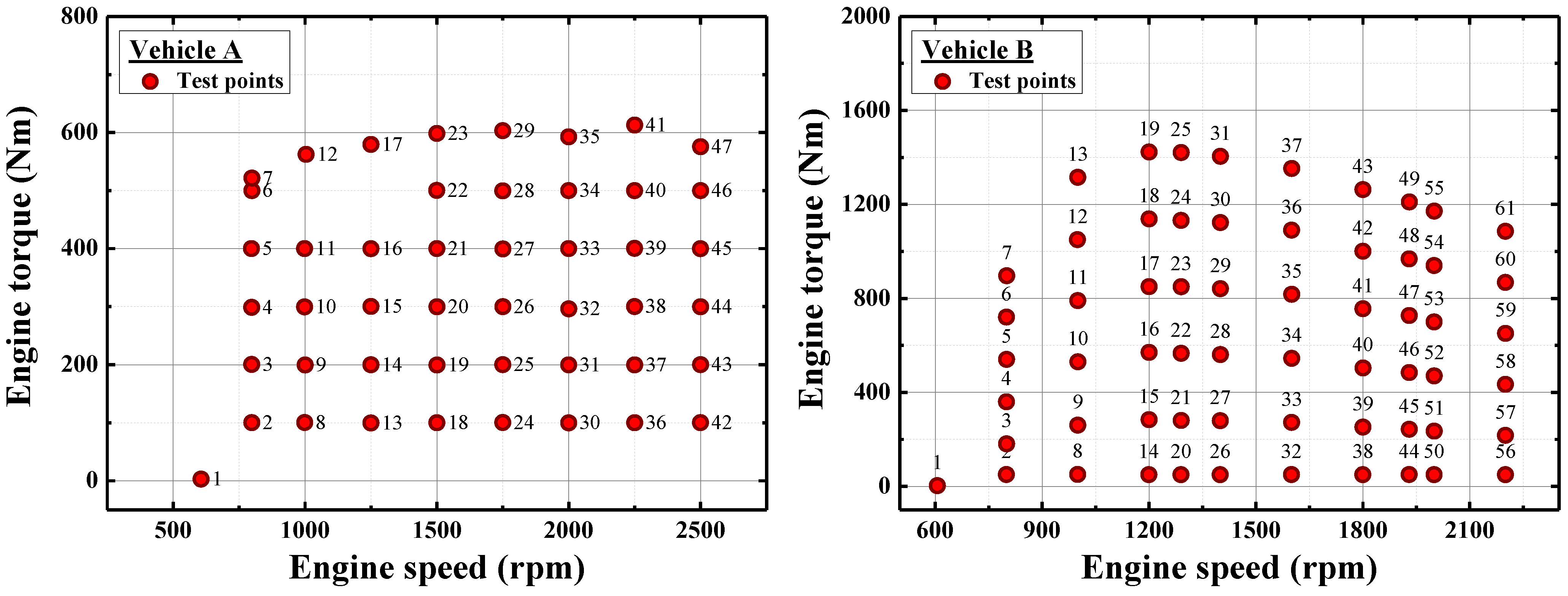
Figure 5. Fuel consumption map data: (a) Vehicle A (b) Vehicle B.

Figure 5. Fuel consumption map data: (a) Vehicle A (b) Vehicle B.

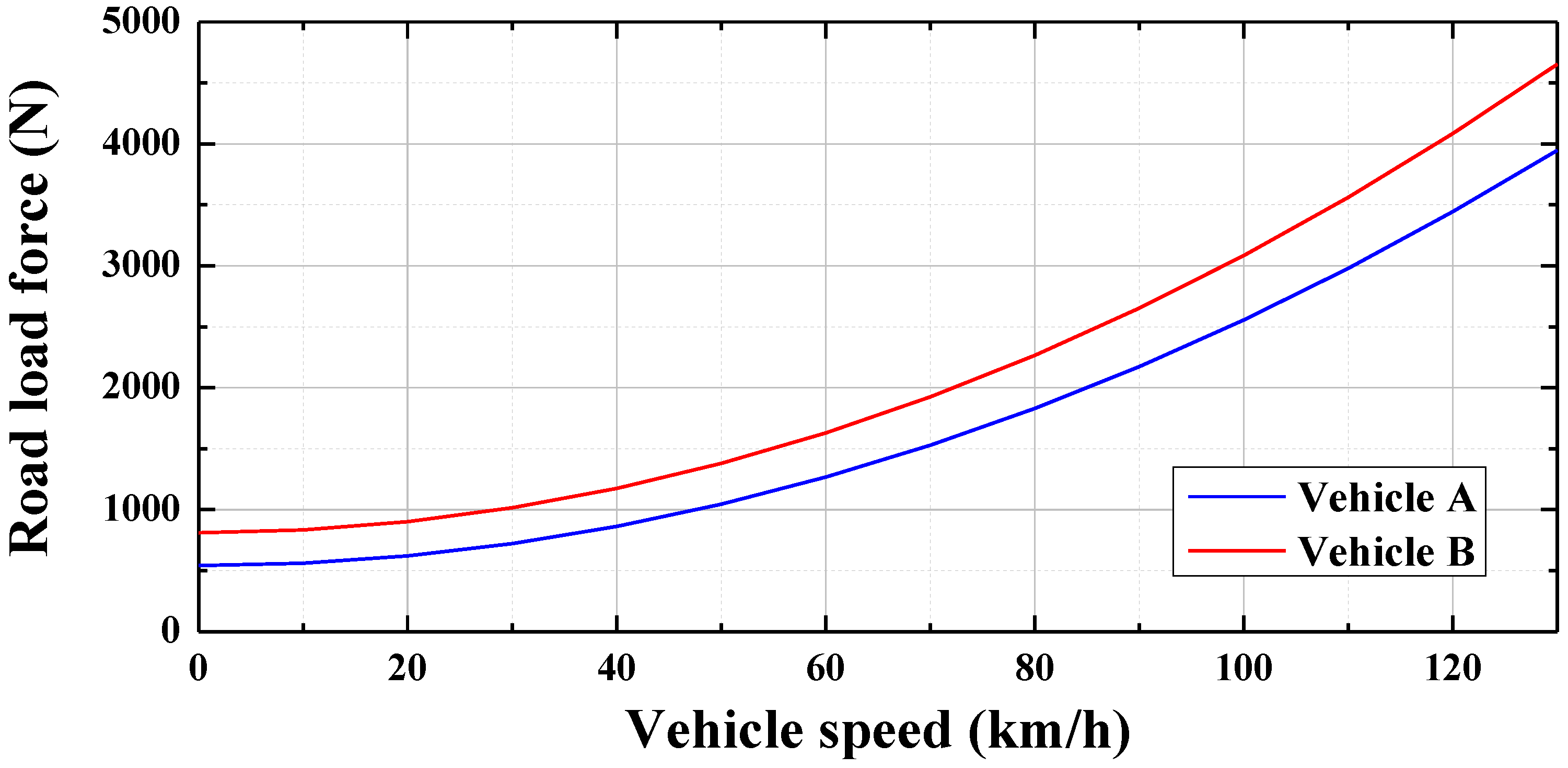
Meanwhile, the chassis dynamometer set-up procedure is important to transfer the exact driving resistance for when the HDV operates in real circumstances. Therefore, prior to the chassis dynamometer test, the road load force of each vehicle should be defined as a three-term polynomial formula in terms of speed as shown in Equation (14) [19,20]:

$$F_{\text{road}}=A{V}^2+BV+C$$

(14)

where V is the vehicle velocity (unit: km/h); and the coastdown coefficients (A, B, C) are determined by test data analysis, which is essentially used as a chassis dynamometer setting. Generally, the road load force consists of air drag, rolling resistance, and mechanical transmission losses. It is preferable to perform the test to determine accurate coast down data. However, the coast down test of the heavy-duty vehicle has some difficult operational requirements to and a longer deceleration distance compared to passenger vehicles [10,21]. For convenience, the coastdown coefficients can be calculated by the Japanese transformation algorithm program. This program contains a calculation routine for air drag and rolling resistance forces, and the road load force is defined as the sum of these two forces. Therefore, the dynamometer inertia setting based on the simulation method was enabled without the vehicle coast down test procedure, as shown in Figure 6 and Table 5.

Figure 6. Example of predicted coastdown results represented by a three-term polynomial curve.

Figure 6. Example of predicted coastdown results represented by a three-term polynomial curve.

Table 5. Coastdown Coefficient results.

Test vehicle	A	B	C
Vehicle A	0.2017	0	593.78
Vehicle B	0.2273	0	811.65

Table 5. Coastdown Coefficient results.

Test vehicle	A	B	C
Vehicle A	0.2017	0	593.78
Vehicle B	0.2273	0	811.65

The total driving resistance force defined as sum of the rolling resistance and aerodynamic resistance force shows a symmetric grape with respect to the y-axis in terms of vehicle speed (rolling resistance was determined by the test vehicle weight and aerodynamic resistance force was proportional to the square of vehicle speed). Thus, the coastdown coefficient value of B determined to be zero. After the chassis dynamometer setting and test vehicle installation procedure, the JE05 mode (Japan, emission test mode) and World Harmonized Vehicle Cycle (WHVC) mode tests [21] for the two vehicle model are conducted. In order to analyze and ensure the actual test mode based on the type of approved driving mode, comparative analysis is conducted between the two data sets. As shown in Figure 7, approved driving mode and actual driving mode show agreement over the whole test time.

Figure 7. Comparison of vehicle profiles between approved driving mode and actual test driving mode and predicted gear position according to time: (a) Vehicle A, JE05 mode; (b) Vehicle A, WHVC mode; (c) Vehicle B, JE05 mode.

Figure 7. Comparison of vehicle profiles between approved driving mode and actual test driving mode and predicted gear position according to time: (a) Vehicle A, JE05 mode; (b) Vehicle A, WHVC mode; (c) Vehicle B, JE05 mode.

Figure 7 also shows the gear position predicted by the Japanese transformation algorithm program. The gear shifting habit can greatly influence vehicle performance, so the gear position should be identically set in both the simulation method and test method. The simulation method is set to automatically determine gear position, whereas the test method has the advantage that the driver can manipulate the gear position of the test vehicle within a certain range. Therefore, the gear position is previously predicted by the Japanese transformation algorithm program, and the actual test should follow this gear position data. Through this process, the relative error induced by the difference of gear position between the simulation and test methods was effectively eliminated. Through the whole procedure, the fuel efficiency test results based on the carbon balance method were obtained as shown in Table 6.

Table 6. Fuel efficiency test results.

Category	Test vehicle	Test cycle	Fuel efficiency (km/L, C_B)
Case 1	Vehicle A	JE05 mode	4.43
Case 2	Vehicle A	WHVC mode	4.76
Case 3	Vehicle B	JE05 mode	3.13

Table 6. Fuel efficiency test results.

Category	Test vehicle	Test cycle	Fuel efficiency (km/L, C_B)
Case 1	Vehicle A	JE05 mode	4.43
Case 2	Vehicle A	WHVC mode	4.76
Case 3	Vehicle B	JE05 mode	3.13

4. Results and Discussion

4.1. Impact of Interpolation Method on Prediction Accuracy of HDV Fuel Efficiency

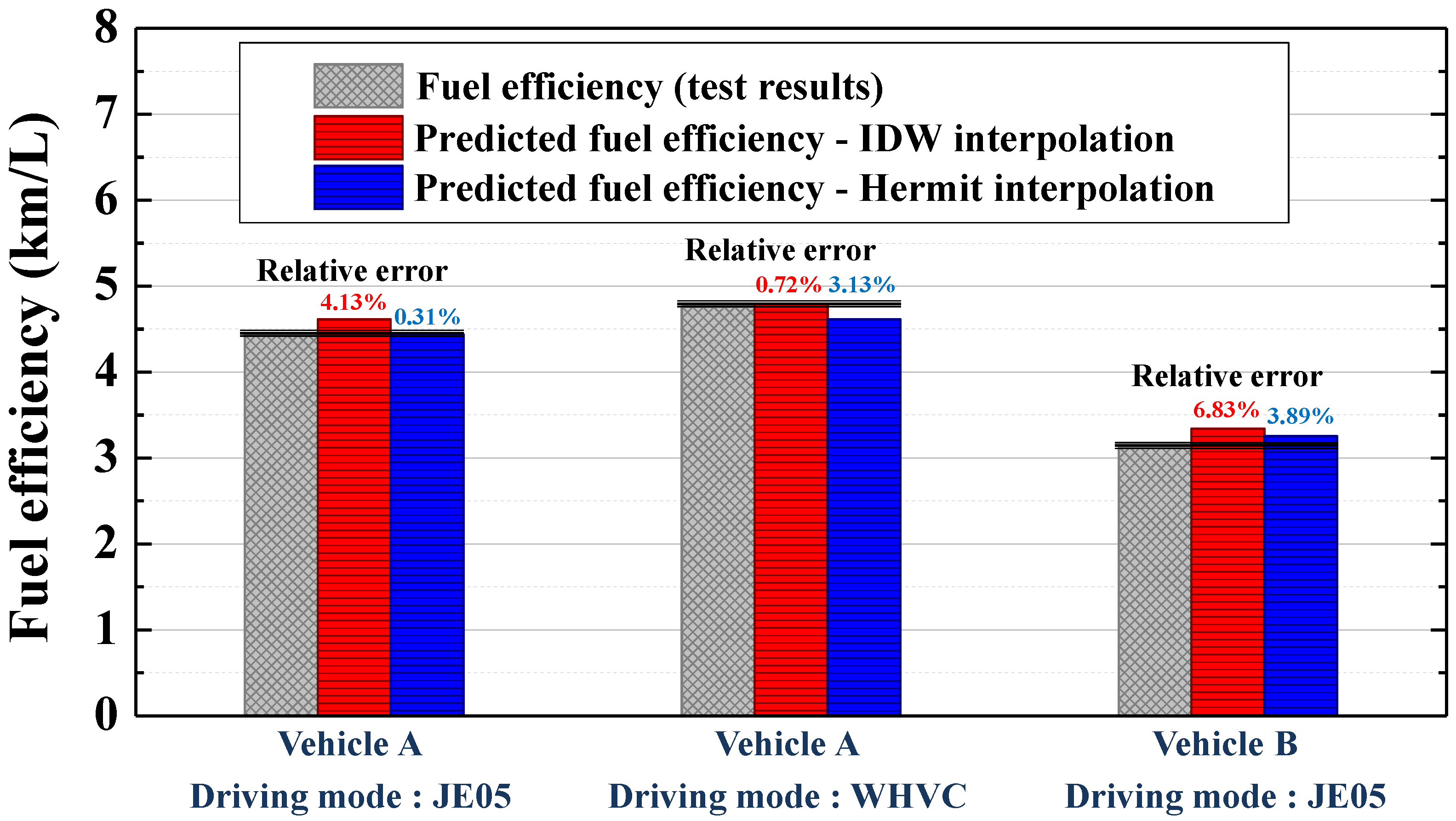
In the present study, six cases (two simulations per test case) were simulated by changing the interpolation method (IDW and Hermite) and calculated results were compared with experimental results as shown in Figure 8 and Table 7. In each case, only the interpolation method was changed, while all other input data remained unchanged against from basic values.

Figure 8. Comparative analysis of the HDV test and predicted fuel efficiency results.

Figure 8. Comparative analysis of the HDV test and predicted fuel efficiency results.

In Figure 8 and Table 7, the predicted results show good agreement with experimental results. Predicted results fuel efficiencies agree well with experiments within ±7% accuracy. These results show that program is reliable in predicting fuel efficiency by adopting main specifications even if users do not enter the detailed information of the vehicle.

When adopting the IDW interpolation method, the predicted results show a higher relative error range (within 6.9% accuracy), whereas the error range is reduced by implementing the Hermite interpolation method (within ±3.9% accuracy). Case 2 (Vehicle A, WHVC mode) shows higher prediction accuracy with the IDW interpolation method, but the overall prediction accuracy is stable when applying the Hermite method. The main cause of these discrepancies is that the gradient information is considered with or without the interpolation method.

Table 7. Predicted fuel efficiency results and relative error between simulation and test.

Category	Test vehicle	Test Cycle	Fuel efficiency (km/L, C_B)	Interpolation method	Predicted fuel efficiency (km/L)	Relative error (%)
Case 1	Vehicle A	JE05 mode	4.43	IDW	4.61	4.13
				Hermite	4.44	0.31
Case 2	Vehicle A	WHVC mode	4.76	IDW	4.79	0.72
				Hermite	4.61	3.13
Case 3	Vehicle B	JE05 mode	3.13	IDW	3.34	6.83
				Hermite	3.25	3.89

Table 7. Predicted fuel efficiency results and relative error between simulation and test.

Category	Test vehicle	Test Cycle	Fuel efficiency (km/L, C_B)	Interpolation method	Predicted fuel efficiency (km/L)	Relative error (%)
Case 1	Vehicle A	JE05 mode	4.43	IDW	4.61	4.13
				Hermite	4.44	0.31
Case 2	Vehicle A	WHVC mode	4.76	IDW	4.79	0.72
				Hermite	4.61	3.13
Case 3	Vehicle B	JE05 mode	3.13	IDW	3.34	6.83
				Hermite	3.25	3.89

The Hermite interpolation method reflects the gradient information of both endpoints to create the third-order equations, whereas the IDW interpolation method does not. Thus, the predicted fuel efficiency results using the IDW interpolation method are generally an overestimate, as shown in Figure 9.

Figure 9. Difference in prediction accuracy between Hermite and IDW interpolation method.

Figure 9. Difference in prediction accuracy between Hermite and IDW interpolation method.

4.2. Impact of Number of Data Points on Prediction Accuracy of HDV’s Fuel Efficiency

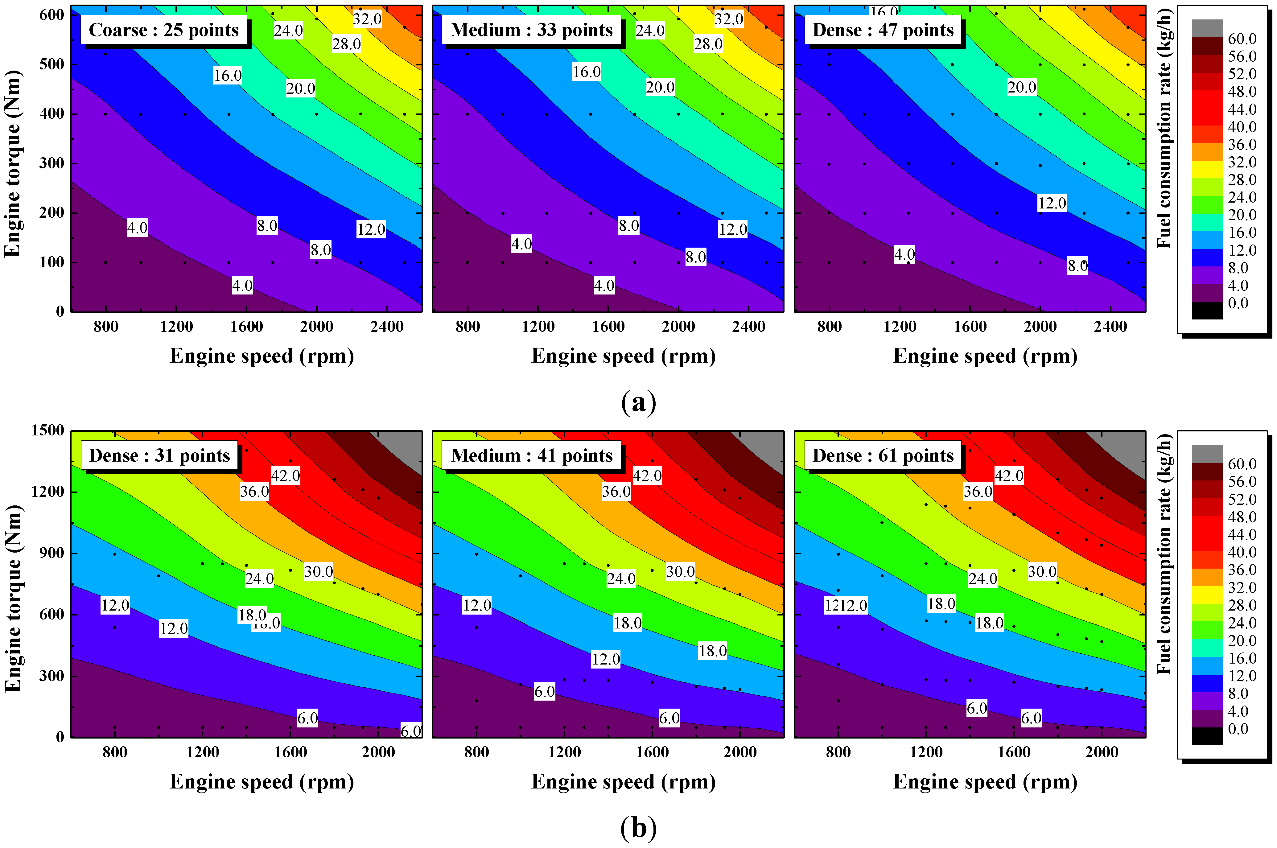
This section describes and implements the three types of fuel efficiency map (coarse, medium, and dense) as input data to determine how the number of fuel consumption data impacts prediction accuracy. Figure 10 shows the fuel efficiency map composed of all the data that originated from test results. Medium and coarse fuel efficiency maps were created by eliminating the specific data line. The main reason for changing the number of data point is to check how the map data density impact on prediction accuracy. If simulation do not shows the advanced results even though the number of data point is increased, it will be a good reference that coarse type of maps (30-points) is enough to conduct the simulation, time and cost saving is expected by reducing chassis dynamo test conditions. The color shading is added in map to enhance understanding of the map data composition (Figure 3 and Figure 4 also conduct the color shading process).

Figure 10. Difference in predicted fuel consumption rate as changes in the reference data points (IDW interpolation method): (a) Vehicle A (b) Vehicle B.

Figure 10. Difference in predicted fuel consumption rate as changes in the reference data points (IDW interpolation method): (a) Vehicle A (b) Vehicle B.

In the process of creating coarse and medium fuel efficiency maps, elimination of the min/max engine torque data line is avoided in order to avoid inaccurate calculation results. The implementation of specific revolution-torque combination data that exceed the fuel efficiency map data range in the calculation process may cause serious errors regardless of the number of total data points.

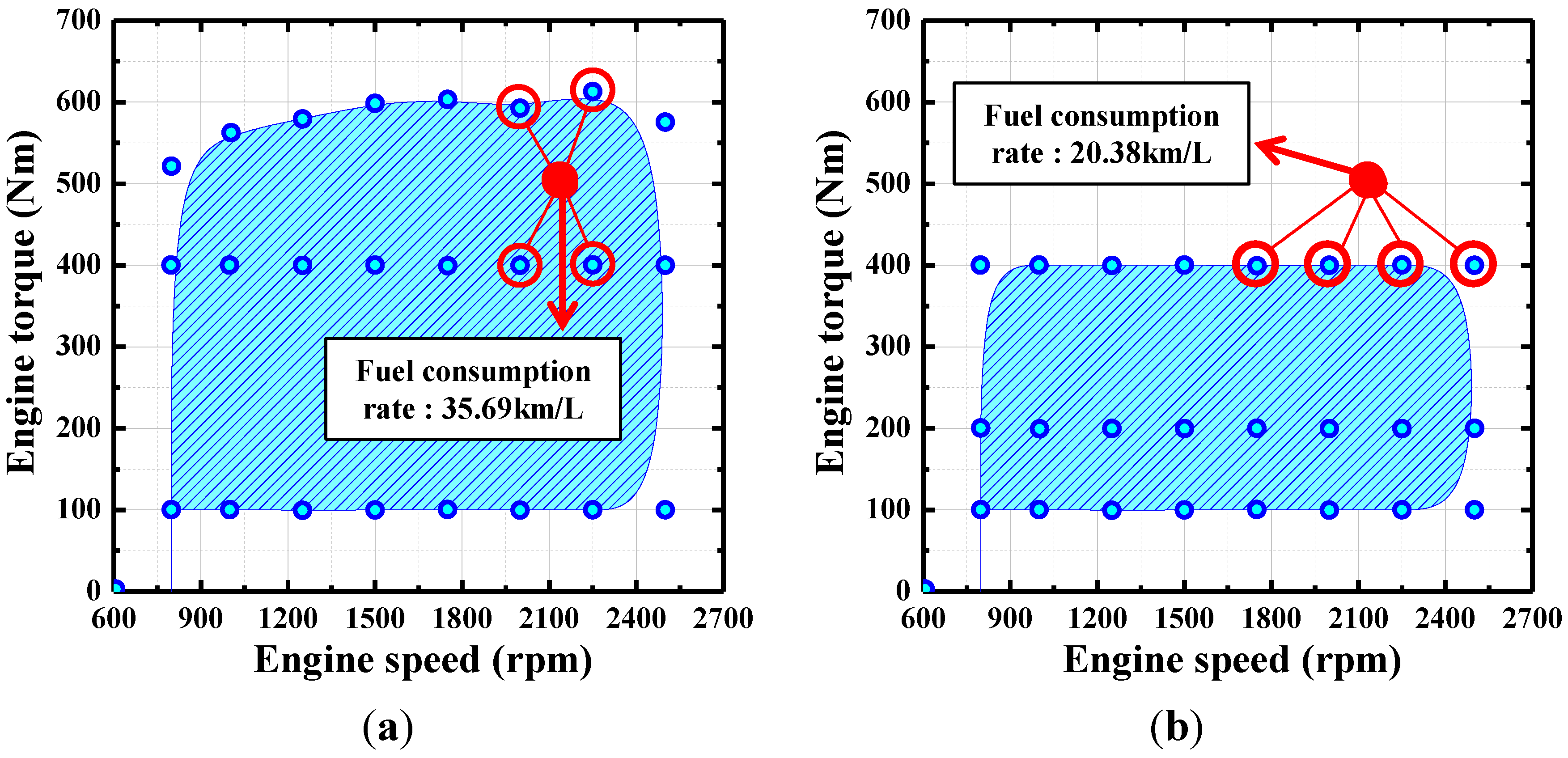
Figure 11 shows the predicted fuel consumption rate at a specific revolution-torque combination point as the reference data points change. Although the interpolation method is fixed, the predicted results present a large gap. It is expected that this gap would be reduced significantly when using the Hermite method, but the elimination of the min/max engine torque data line should be avoided. Therefore, all of the fuel efficiency map data adopted in this study is basically set to contain the threshold data (min/max engine torque data).

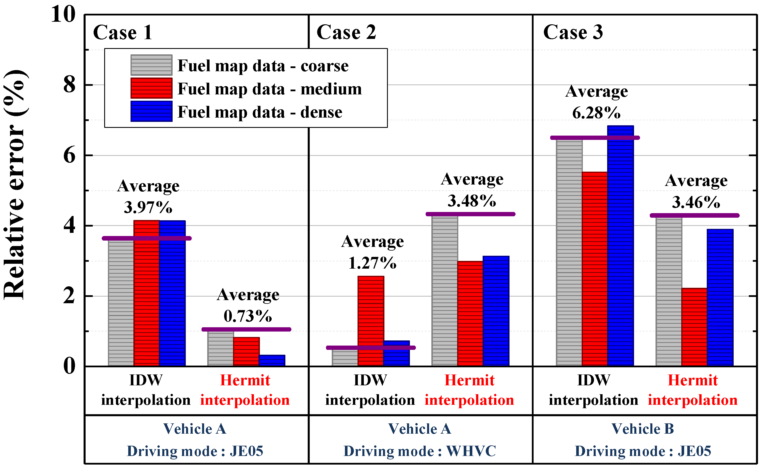
Figure 12 shows the predicted fuel efficiency results obtained by changing the number of fuel efficiency map data points with the input data and interpolation method. The overall prediction accuracy is generally higher when using Hermite interpolation. The predicted results obtained by applying the Hermite interpolation method meet the measured fuel consumption within ±3.5% accuracy, whereas the IDW interpolation method meets the measured fuel consumption within ±6.3%. It means that finer grid is needed to improve the local approximation accuracy of IDW interpolation. However, composing a dense type map has limitation that needs many cost and time consuming; it is obvious that the merit of simulation is become questionable. On average, the Hermite method shows approximately 45% higher prediction accuracy. It can be a problem that Hermite method shows the worse results in case 2, the Hermite method shows the stable prediction results (On average, the relative error converged in 3.5%) regardless of calculation conditions whereas IDW method shows about 4% and 6% of errors in case 1 and 3. Thus, it is desirable to implement the Hermite interpolation method in further results. Meanwhile, the impact of changing the data points on fuel efficiency prediction results shows no particular tendency. Moreover, in some cases, the prediction accuracy decreases slightly despite the increasing data density. This problem is caused by nonlinear characteristic exist in actual fuel consumption map data. The ideal fuel consumption map explained in this paper represents the shape of the curve that slightly downward (Figure 3, Figure 4, and Figure 10). These shapes are visibly enabled by using smoothing method, the actual map data containing the irregularly bending regions that cause inaccurate prediction results. It can be partially complemented by applying Hermite interpolation method if gradient is not drastically changed, the IDW method do not solve this problem unless the composition of data point very fine enough to neglect the gradient information. Thus, the prediction accuracy is not impacted by fuel efficiency data density and the fuel efficiency map would not necessarily need to have a high density, and around 30 data points is sufficient for high prediction accuracy unless the threshold data (min/max engine torque data) was eliminated.

Figure 11. Difference in predicted fuel consumption rate with changes in the reference data point (IDW interpolation method): (a) appropriate fuel efficiency map composition (b) inappropriate fuel efficiency map composition.

Figure 11. Difference in predicted fuel consumption rate with changes in the reference data point (IDW interpolation method): (a) appropriate fuel efficiency map composition (b) inappropriate fuel efficiency map composition.

Figure 12. Change of predicted fuel efficiency results with variation of the number of data points and interpolation method.

Figure 12. Change of predicted fuel efficiency results with variation of the number of data points and interpolation method.

4.3. Sensitivity Analysis Study

Some variables such as engine performance, vehicle specifications, and transmission efficiency greatly influence HDV fuel efficiency. To perform a more detailed analysis, sensitivity studies were conducted by varying the input data value. The parameters expected to affect HDV fuel efficiency can be divided into three categories as shown in Table 8 [17].

Table 8. The categorization of main input parameters impact on HDV fuel efficiency.

Category	Input parameter
Vehicle performance	Driving force, Maximum engine torque, Fuel efficiency map
Transmission	Final gear ratio, Transmission efficiency
Vehicle specification	Drag & rolling resistance coefficient, Vehicle height (width), Vehicle weight

Table 8. The categorization of main input parameters impact on HDV fuel efficiency.

Category	Input parameter
Vehicle performance	Driving force, Maximum engine torque, Fuel efficiency map
Transmission	Final gear ratio, Transmission efficiency
Vehicle specification	Drag & rolling resistance coefficient, Vehicle height (width), Vehicle weight

In these variations, one parameter was changed while all others remained unchanged in order to more sensitively analyze the impact of each input parameter on HDV fuel efficiency. These analysis approaches are a little unrealistic because changes in any single parameter inevitably entail additional changes in the associated factors. Thus, the results of this section require the assumption that changing a single parameter does not necessarily represent realistic fuel consumption behavior. However, the sensitivity analysis is expected to quantitatively show which parameters have the greater influence on HDV fuel efficiency. Simulations with changes to the input parameter at a certain rate (±1%, ±3%, ±5% and ±10%) were conducted for all test cases, and the calculated fuel efficiency results were compared with the test results. According to Mammetti et al. [22], it is reported that the most impacting factors on HDV fuel efficiency is engine efficiency (rank 1), aerodynamic (rank 2) and rolling resistance (rank 3). This study conducts the fuel efficiency test with changing the tire which has different rolling resistance coefficients and reveals the rolling resistance coefficients can impact the HDV fuel efficiency more than 15%. With considering that impact factor of rolling resistance coefficient is lower than drag and engine efficiency factors [22], it is appropriate to conduct the study with changing these parameters at range of ±10%.

Table 9, Table 10 and Table 11 show the predicted fuel efficiency and relative error as input parameter variations. In order to calculate the relative error, the predicted results calculated by adopting the Hermite interpolation method were selected as baseline cases.

• Case 1 - Vehicle A, JE05 mode, Fuel efficiency: 4.44 km/L
• Case 2 - Vehicle A, WHVC mode, Fuel efficiency: 4.61 km/L
• Case 3 - Vehicle B, JE05 mode, Fuel efficiency: 3.25 km/L

As expected, the fuel efficiency results increased with decreases in the driving force, fuel consumption map data, drag and rolling resistance coefficient, vehicle size, and weight value. The effect of the final gear ratio and maximum engine torque parameters are expected to have a smaller impact on fuel efficiency than other parameters and do not show a particular tendency.

Table 9. Relative changes of the predicted fuel efficiency results compared to baseline case—case 1.

Input parameter	VehicleA JE05 mode	−10%	−5%	−3%	−1%	0%	1%	3%	5%	10%
1. Driving force (N)	fuel eff. (km/L)	4.82	4.63	4.55	4.48	4.44	4.41	4.34	4.24	4.08
	change rate (%)	8.42	4.27	2.45	0.92	0.00	−0.69	−2.36	−4.66	−8.18
2. Maximum engine torque (Nm)	fuel eff. (km/L)	4.35	4.39	4.43	4.44	4.44	4.45	4.45	4.46	4.47
	change rate (%)	−2.06	−1.29	−0.32	−0.02	0.00	0.18	0.20	0.34	0.58
3. Fuel consumption map data (km/L)	fuel eff. (km/L)	4.94	4.68	4.58	4.49	4.44	4.40	4.31	4.23	4.04
	change rate (%)	11.11	5.26	3.09	1.01	0.00	−0.99	−2.91	−4.76	−9.09
4. Final gear ratio (-)	fuel eff. (km/L)	4.44	4.45	4.44	4.45	4.44	4.44	4.42	4.42	4.35
	change rate (%)	−0.03	0.05	−0.03	0.20	0.00	−0.06	−0.46	−0.60	−2.15
5. Drag coefficient (-)	fuel eff. (km/L)	4.52	4.48	4.46	4.45	4.44	4.44	4.42	4.41	4.37
	change rate (%)	1.61	0.78	0.44	0.15	0.00	−0.17	−0.51	−0.84	−1.70
6. Rolling resistance coefficient (-)	fuel eff. (km/L)	4.50	4.47	4.46	4.45	4.44	4.44	4.43	4.41	4.38
	change rate (%)	1.36	0.66	0.35	0.13	0.00	−0.14	−0.41	−0.76	−1.42
7. Frontal area (m2)	fuel eff. (km/L)	4.52	4.48	4.46	4.45	4.44	4.44	4.42	4.41	4.37
	change rate (%)	1.64	0.82	0.45	0.16	0.00	−0.17	−0.53	−0.87	−1.76
8. Gross vehicle weight (kg)	fuel eff. (km/L)	4.66	4.55	4.50	4.47	4.44	4.42	4.38	4.29	4.18
	change rate (%)	4.94	2.36	1.37	0.66	0.00	−0.44	−1.37	−3.56	−5.84
Transmission efficiency (direct gear)	fuel eff. (km/L)	4.25	4.34	4.38	4.42	4.44	4.46	4.50	4.54	4.63
	change rate (%)	−4.38	−2.26	−1.40	−0.45	0.00	0.38	1.33	2.11	4.15
Transmission efficiency (final gear)	fuel eff. (km/L)	4.04	4.23	4.33	4.41	4.44	4.48	4.55	4.62	4.79
	change rate (%)	−9.16	−4.82	−2.52	−0.70	0.00	0.90	2.40	3.90	7.68
Transmission efficiency (other gear)	fuel eff. (km/L)	4.23	4.33	4.39	4.43	4.44	4.47	4.49	4.52	4.59
	change rate (%)	−4.77	−2.63	−1.15	−0.25	0.00	0.52	1.09	1.77	3.33

Table 9. Relative changes of the predicted fuel efficiency results compared to baseline case—case 1.

Input parameter	VehicleA JE05 mode	−10%	−5%	−3%	−1%	0%	1%	3%	5%	10%
1. Driving force (N)	fuel eff. (km/L)	4.82	4.63	4.55	4.48	4.44	4.41	4.34	4.24	4.08
	change rate (%)	8.42	4.27	2.45	0.92	0.00	−0.69	−2.36	−4.66	−8.18
2. Maximum engine torque (Nm)	fuel eff. (km/L)	4.35	4.39	4.43	4.44	4.44	4.45	4.45	4.46	4.47
	change rate (%)	−2.06	−1.29	−0.32	−0.02	0.00	0.18	0.20	0.34	0.58
3. Fuel consumption map data (km/L)	fuel eff. (km/L)	4.94	4.68	4.58	4.49	4.44	4.40	4.31	4.23	4.04
	change rate (%)	11.11	5.26	3.09	1.01	0.00	−0.99	−2.91	−4.76	−9.09
4. Final gear ratio (-)	fuel eff. (km/L)	4.44	4.45	4.44	4.45	4.44	4.44	4.42	4.42	4.35
	change rate (%)	−0.03	0.05	−0.03	0.20	0.00	−0.06	−0.46	−0.60	−2.15
5. Drag coefficient (-)	fuel eff. (km/L)	4.52	4.48	4.46	4.45	4.44	4.44	4.42	4.41	4.37
	change rate (%)	1.61	0.78	0.44	0.15	0.00	−0.17	−0.51	−0.84	−1.70
6. Rolling resistance coefficient (-)	fuel eff. (km/L)	4.50	4.47	4.46	4.45	4.44	4.44	4.43	4.41	4.38
	change rate (%)	1.36	0.66	0.35	0.13	0.00	−0.14	−0.41	−0.76	−1.42
7. Frontal area (m2)	fuel eff. (km/L)	4.52	4.48	4.46	4.45	4.44	4.44	4.42	4.41	4.37
	change rate (%)	1.64	0.82	0.45	0.16	0.00	−0.17	−0.53	−0.87	−1.76
8. Gross vehicle weight (kg)	fuel eff. (km/L)	4.66	4.55	4.50	4.47	4.44	4.42	4.38	4.29	4.18
	change rate (%)	4.94	2.36	1.37	0.66	0.00	−0.44	−1.37	−3.56	−5.84
Transmission efficiency (direct gear)	fuel eff. (km/L)	4.25	4.34	4.38	4.42	4.44	4.46	4.50	4.54	4.63
	change rate (%)	−4.38	−2.26	−1.40	−0.45	0.00	0.38	1.33	2.11	4.15
Transmission efficiency (final gear)	fuel eff. (km/L)	4.04	4.23	4.33	4.41	4.44	4.48	4.55	4.62	4.79
	change rate (%)	−9.16	−4.82	−2.52	−0.70	0.00	0.90	2.40	3.90	7.68
Transmission efficiency (other gear)	fuel eff. (km/L)	4.23	4.33	4.39	4.43	4.44	4.47	4.49	4.52	4.59
	change rate (%)	−4.77	−2.63	−1.15	−0.25	0.00	0.52	1.09	1.77	3.33

The effect of the transmission efficiency variations on the fuel efficiency of HDVs is expected to be greater than other parameters, as noted in Table 9. In the case of the passenger car, the actual transmission developments tend toward various directions, such as automatic transmission, dual clutch transmission, high-efficiency transmissions, and early torque converter lockup [23]. However, this study focused only on the power transfer efficiency of the transmission; the ±10% change in transfer efficiency is unrealistic without adopting the newly developed technologies. Generally, an HDV has been implemented with manual transmissions due to technical limitations but some bus models now also implements the automatic transmissions. Therefore, it is an important to consider transmission efficiency on further simulation studies. In this study area, the result data related to transmission efficiency are appropriate for use as a reference data, and more sufficient data is needed to reflect this trend in simulation.

Table 10. Relative changes of the predicted fuel efficiency results compared to baseline case—case 2.

Input parameter	VehicleA WHVC mode	−10%	−5%	−3%	−1%	0%	1%	3%	5%	10%
1. Driving force (N)	fuel eff. (km/L)	5.00	4.78	4.72	4.64	4.61	4.57	4.48	4.41	4.25
	change rate (%)	8.54	3.71	2.31	0.54	0.00	−0.92	−2.75	−4.26	−7.83
2. Maximum engine torque (Nm)	fuel eff. (km/L)	4.57	4.58	4.58	4.60	4.61	4.60	4.61	4.61	4.64
	change rate (%)	−0.99	−0.62	−0.62	−0.18	0.00	−0.16	−0.06	−0.01	0.57
3. Fuel consumption map data (km/L)	fuel eff. (km/L)	5.12	4.85	4.75	4.66	4.61	4.57	4.48	4.39	4.19
	change rate (%)	11.11	5.26	3.09	1.01	0.00	−0.99	−2.91	−4.76	−9.09
4. Final gear ratio (-)	fuel eff. (km/L)	4.64	4.64	4.62	4.62	4.61	4.59	4.57	4.55	4.46
	change rate (%)	0.65	0.63	0.17	0.20	0.00	−0.55	−0.93	−1.36	−3.30
5. Drag coefficient (-)	fuel eff. (km/L)	4.72	4.67	4.64	4.62	4.61	4.60	4.57	4.55	4.49
	change rate (%)	2.39	1.22	0.71	0.19	0.00	−0.23	−0.85	−1.32	−2.57
6. Rolling resistance coefficient (-)	fuel eff. (km/L)	4.68	4.64	4.63	4.62	4.61	4.60	4.58	4.57	4.53
	change rate (%)	1.50	0.70	0.42	0.13	0.00	−0.14	−0.60	−0.90	−1.68
7. Frontal area (m2)	fuel eff. (km/L)	4.72	4.67	4.65	4.62	4.61	4.60	4.57	4.55	4.49
	change rate (%)	2.47	1.26	0.75	0.21	0.00	−0.24	−0.86	−1.39	−2.69
8. Gross vehicle weight (kg)	fuel eff. (km/L)	4.81	4.68	4.64	4.63	4.61	4.58	4.53	4.49	4.39
	change rate (%)	4.35	1.52	0.68	0.40	0.00	−0.61	−1.73	−2.54	−4.74

Table 10. Relative changes of the predicted fuel efficiency results compared to baseline case—case 2.

Input parameter	VehicleA WHVC mode	−10%	−5%	−3%	−1%	0%	1%	3%	5%	10%
1. Driving force (N)	fuel eff. (km/L)	5.00	4.78	4.72	4.64	4.61	4.57	4.48	4.41	4.25
	change rate (%)	8.54	3.71	2.31	0.54	0.00	−0.92	−2.75	−4.26	−7.83
2. Maximum engine torque (Nm)	fuel eff. (km/L)	4.57	4.58	4.58	4.60	4.61	4.60	4.61	4.61	4.64
	change rate (%)	−0.99	−0.62	−0.62	−0.18	0.00	−0.16	−0.06	−0.01	0.57
3. Fuel consumption map data (km/L)	fuel eff. (km/L)	5.12	4.85	4.75	4.66	4.61	4.57	4.48	4.39	4.19
	change rate (%)	11.11	5.26	3.09	1.01	0.00	−0.99	−2.91	−4.76	−9.09
4. Final gear ratio (-)	fuel eff. (km/L)	4.64	4.64	4.62	4.62	4.61	4.59	4.57	4.55	4.46
	change rate (%)	0.65	0.63	0.17	0.20	0.00	−0.55	−0.93	−1.36	−3.30
5. Drag coefficient (-)	fuel eff. (km/L)	4.72	4.67	4.64	4.62	4.61	4.60	4.57	4.55	4.49
	change rate (%)	2.39	1.22	0.71	0.19	0.00	−0.23	−0.85	−1.32	−2.57
6. Rolling resistance coefficient (-)	fuel eff. (km/L)	4.68	4.64	4.63	4.62	4.61	4.60	4.58	4.57	4.53
	change rate (%)	1.50	0.70	0.42	0.13	0.00	−0.14	−0.60	−0.90	−1.68
7. Frontal area (m2)	fuel eff. (km/L)	4.72	4.67	4.65	4.62	4.61	4.60	4.57	4.55	4.49
	change rate (%)	2.47	1.26	0.75	0.21	0.00	−0.24	−0.86	−1.39	−2.69
8. Gross vehicle weight (kg)	fuel eff. (km/L)	4.81	4.68	4.64	4.63	4.61	4.58	4.53	4.49	4.39
	change rate (%)	4.35	1.52	0.68	0.40	0.00	−0.61	−1.73	−2.54	−4.74

Table 11. Relative changes of the predicted fuel efficiency results compared to baseline case—case 3.

Input parameter	VehicleB JE05 mode	−10%	−5%	−3%	−1%	0%	1%	3%	5%	10%
1. Driving force (N)	fuel eff. (km/L)	3.51	3.39	3.34	3.28	3.25	3.23	3.19	3.16	3.03
	change rate (%)	8.08	4.38	2.76	0.73	0.00	−0.60	−1.79	−2.84	−6.67
2. Maximum engine torque (Nm)	fuel eff. (km/L)	3.29	3.31	3.29	3.27	3.25	3.25	3.27	3.26	3.22
	change rate (%)	1.25	1.71	1.17	0.50	0.00	−0.02	0.43	0.14	−1.00
3. Fuel consumption map data (km/L)	fuel eff. (km/L)	3.61	3.42	3.35	3.28	3.25	3.22	3.16	3.10	2.96
	change rate (%)	11.11	5.26	3.09	1.01	0.00	−0.99	−2.91	−4.76	−9.09
4. Final gear ratio (-)	fuel eff. (km/L)	3.28	3.26	3.28	3.27	3.25	3.24	3.25	3.26	3.25
	change rate (%)	1.01	0.35	0.76	0.59	0.00	−0.37	0.06	0.38	0.06
5. Drag coefficient (-)	fuel eff. (km/L)	3.29	3.27	3.26	3.26	3.25	3.25	3.24	3.23	3.21
	change rate (%)	1.32	0.67	0.34	0.12	0.00	−0.13	−0.43	−0.65	−1.27
6. Rolling resistance coefficient (-)	fuel eff. (km/L)	3.30	3.28	3.27	3.26	3.25	3.25	3.24	3.23	3.22
	change rate (%)	1.59	0.80	0.48	0.11	0.00	−0.16	−0.41	−0.63	−1.00
7. Frontal area (m2)	fuel eff. (km/L)	3.30	3.27	3.26	3.26	3.25	3.25	3.24	3.23	3.21
	change rate (%)	1.38	0.68	0.37	0.13	0.00	−0.14	−0.45	−0.67	−1.32
8. Gross vehicle weight (kg)	fuel eff. (km/L)	3.46	3.37	3.33	3.27	3.25	3.24	3.21	3.18	3.09
	change rate (%)	6.32	3.70	2.29	0.56	0.00	−0.41	−1.34	−2.17	−4.92

Table 11. Relative changes of the predicted fuel efficiency results compared to baseline case—case 3.

Input parameter	VehicleB JE05 mode	−10%	−5%	−3%	−1%	0%	1%	3%	5%	10%
1. Driving force (N)	fuel eff. (km/L)	3.51	3.39	3.34	3.28	3.25	3.23	3.19	3.16	3.03
	change rate (%)	8.08	4.38	2.76	0.73	0.00	−0.60	−1.79	−2.84	−6.67
2. Maximum engine torque (Nm)	fuel eff. (km/L)	3.29	3.31	3.29	3.27	3.25	3.25	3.27	3.26	3.22
	change rate (%)	1.25	1.71	1.17	0.50	0.00	−0.02	0.43	0.14	−1.00
3. Fuel consumption map data (km/L)	fuel eff. (km/L)	3.61	3.42	3.35	3.28	3.25	3.22	3.16	3.10	2.96
	change rate (%)	11.11	5.26	3.09	1.01	0.00	−0.99	−2.91	−4.76	−9.09
4. Final gear ratio (-)	fuel eff. (km/L)	3.28	3.26	3.28	3.27	3.25	3.24	3.25	3.26	3.25
	change rate (%)	1.01	0.35	0.76	0.59	0.00	−0.37	0.06	0.38	0.06
5. Drag coefficient (-)	fuel eff. (km/L)	3.29	3.27	3.26	3.26	3.25	3.25	3.24	3.23	3.21
	change rate (%)	1.32	0.67	0.34	0.12	0.00	−0.13	−0.43	−0.65	−1.27
6. Rolling resistance coefficient (-)	fuel eff. (km/L)	3.30	3.28	3.27	3.26	3.25	3.25	3.24	3.23	3.22
	change rate (%)	1.59	0.80	0.48	0.11	0.00	−0.16	−0.41	−0.63	−1.00
7. Frontal area (m2)	fuel eff. (km/L)	3.30	3.27	3.26	3.26	3.25	3.25	3.24	3.23	3.21
	change rate (%)	1.38	0.68	0.37	0.13	0.00	−0.14	−0.45	−0.67	−1.32
8. Gross vehicle weight (kg)	fuel eff. (km/L)	3.46	3.37	3.33	3.27	3.25	3.24	3.21	3.18	3.09
	change rate (%)	6.32	3.70	2.29	0.56	0.00	−0.41	−1.34	−2.17	−4.92

To more simply analyze and instinctively identify which parameters have a great impact on the simulation results, Figure 13 summarizes the maximum change rates of the predicted fuel efficiency according to input data changes (±10%).

Figure 13. Maximum change rate of the predicted fuel efficiency according to input parameter changes.

Figure 13. Maximum change rate of the predicted fuel efficiency according to input parameter changes.

The impact of variation of each parameter on the maximum change rate of the fuel efficiency results shows different tendencies, although the maximum change rates of the input parameters are fixed. It is shown that 10% changes in the input parameter, increase or decrease the fuel efficiency by at least 1.3% compared with the reference value. The maximum engine torque data had little impact (1%–2%) on the results regardless of the vehicle model or driving mode, unlike other parameters. This indicates that the engine modes were not set on the critical area in the case of the HDV drive on JE05 and WHVC modes. If the driving mode needs harsher conditions or road gradient data considered in simulation, it is expected that the maximum engine torque will have a greater impact on the HDV fuel efficiency. Meanwhile, the influence of the final gear ratio on HDV fuel efficiency shows the similar level (about 1%–3%) with drag and rolling resistance parameter. As the final gear ratio higher or lower, the engine speed also has to be proportionally changed or gear shifting points are switched to make an adequate vehicle speed at same driving modes. Anyway, it is obvious that final gear ratio read to the change of engine operating condition and fuel consumption ratio in whole driving time. Some parameters such as drag coefficient and frontal area (which is also related to drag resistance) have a great influence (about 2%–3%) in the case of vehicle A, while vehicle B is the less influenced by these parameter changes (about 1%–2%). According to the available data, the required drag and rolling resistance force relative to the overall engine power is higher for vehicle A than for vehicle B. Vehicle B has higher inertia than vehicle A because the momentum of an HDV is generally proportional to the gross weight. The increasing momentum means an increase of the characteristics maintaining the existing condition; therefore, vehicle B is little affected by changing drag forces.

Meanwhile, the eight parameters are ranked based on the maximum change rate of the fuel efficiency as follows:

• Fuel consumption map data
• Driving force
• Gross vehicle weight
• Frontal size (changing in vehicle height and width)
• Drag coefficient
• Rolling resistance coefficient
• Final gear ratio
• Maximum engine torque

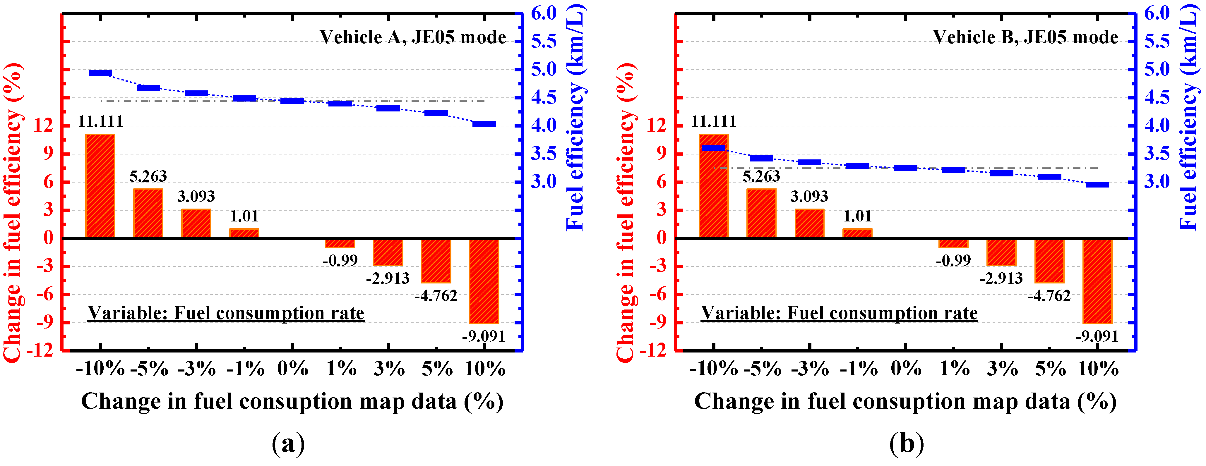
The fuel consumption map data has the greatest impact on HDV fuel efficiency. If the fuel consumption efficiency is improved by 10%, it is expected that the fuel efficiency will increase by 11.1% regardless of the vehicle model and driving mode, as shown in Figure 14. In past years, most research on HDV mainly focused on engine performance, but newly developed HDV’s engines have challenges in that they must meet both future emission regulations and customer requirements to maintain or advance engine performance. Theoretically, reducing the fuel consumption rate while maintaining engine performance at all engine torque-revolution combination points is the best way to improve fuel efficiency. Realistic approach, however, the implementation of the advanced technologies (reducing heat and mechanical friction loss, turbocharging, powertrain optimization, etc.) and engine and powertrain downsizing are potential keys to increasing fuel efficiency. According to the report by Frost & Sullivan, it is expected that HDV engine downsizing with implementation of advanced technologies could reduce fuel consumption and emissions by about 20% [24].

Figure 14. Change of the predicted fuel efficiency results with variation of the fuel consumption map data: (a) Vehicle A, JE05 mode (b) Vehicle B, JE05 mode.

Figure 14. Change of the predicted fuel efficiency results with variation of the fuel consumption map data: (a) Vehicle A, JE05 mode (b) Vehicle B, JE05 mode.

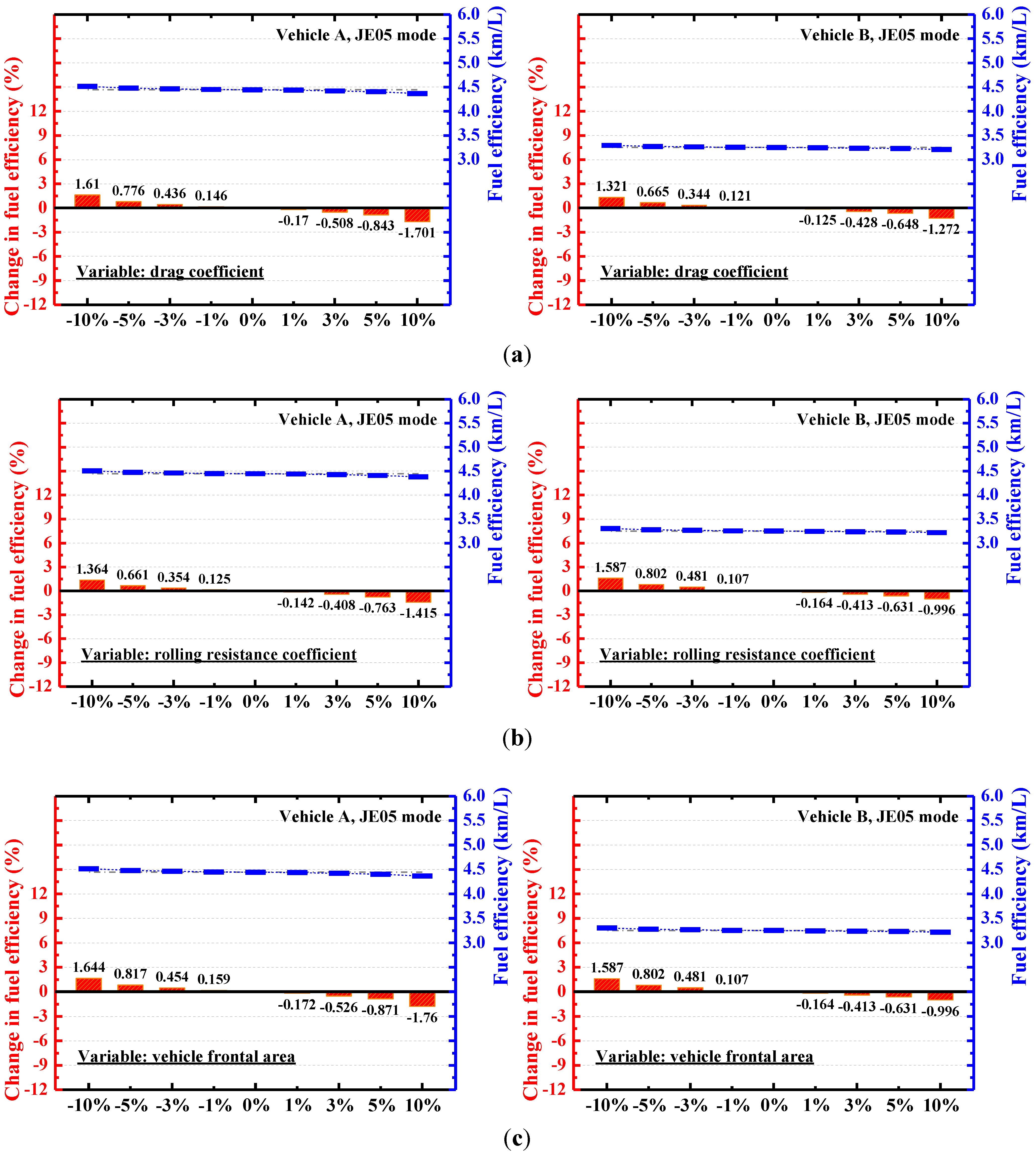
The results show that the driving force defined as the sum of the running resistance force (air drag, rolling resistance) and acceleration force also has a great impact on fuel efficiency. It is a natural outcome that HDV driving force has significant impact on fuel efficiency (about 8%–9%). The acceleration force is fixed without reducing the vehicle weight, and reducing the drag and rolling resistance force is an appropriate way to improve the fuel efficiency. Based on the data as shown in Figure 15, a 2%–3.5% reduction in fuel consumption is expected for a 10% reduction in the drag (or frontal area) and rolling resistance coefficient.

Figure 15. Change of the predicted fuel efficiency results with variation of the drag resistance, rolling resistance and frontal area of HDV: (a) drag coefficient (b) rolling resistance coefficient (c) vehicle frontal area.

Figure 15. Change of the predicted fuel efficiency results with variation of the drag resistance, rolling resistance and frontal area of HDV: (a) drag coefficient (b) rolling resistance coefficient (c) vehicle frontal area.

Figure 16 shows the effect of changes in the gross vehicle weight. Fuel efficiency increased as gross vehicle weight decreased. On average, the HDV fuel efficiency shows a high rate of increase for a 10% reduction in vehicle weight. The rate of increase is slightly higher for vehicle B (about 6%) than vehicle A (about 5%), which indicates that the fuel efficiency of lighter vehicles is significantly affected by vehicle weight.

Figure 16. Change of the predicted fuel efficiency results with variation of the gross vehicle weight.

Figure 16. Change of the predicted fuel efficiency results with variation of the gross vehicle weight.

With the exception of three parameters (fuel consumption map data, driving force and vehicle mass), the change rate of fuel efficiency converged at 4% regardless of the driving mode. However, these factors may be important keys to meet future regulation of HDV fuel efficiency. All of the parameter variation cases (max/min: ±10%) implemented in this study show minimum fuel efficiency changes of about 1%. Therefore, considerations and analysis of how the diverse parameters impact fuel efficiency are necessary in future studies.

4. Conclusions

The present study analyzed the Japanese transformation algorithm program architecture and validated the prediction accuracy of the fuel efficiency results by comparison with chassis dynamometer test results. Furthermore, the influences of the interpolation method and the number of fuel efficiency map data points on prediction accuracy determined which interpolation method and data type are appropriate in these studies. Finally, sensitivity analysis was conducted to determine which parameters have a great impact on the HDV fuel efficiency results. From these studies, the conclusions of the present study can be summarized as follows:

(1)

In the case of identically set gear position in the simulation method and test method, the Japanese transformation algorithm program shows good prediction accuracy. Compared with experimental results data, the error range converged to 7% regardless of the interpolation method. However, the predicted results were more accurate when implementing the Hermite interpolation method (converged to ±3%) compared with IDW interpolation (converged in ±7%). This difference in prediction accuracy between interpolation methods reflects the gradient information. Based on the results data, the IDW interpolation method generally tends to yield an overestimate.

(2)

Three types of fuel efficiency maps (coarse, medium, and dense) were created and implemented in simulation. If the fuel efficiency map covers all driving modes and meets the basic requirements proposed by the Committee for Natural Resource and Energy (CNRE), the prediction accuracy of fuel efficiency is not influenced by fuel efficiency data density. Therefore, the fuel efficiency map consisting of high density test data is not necessarily needed in these studies. Considering the time consumption and test cost, it is appropriate to create a fuel efficiency map as a combination of 30 points, which is enough to achieve acceptable prediction results.

(3)

The analysis study was performed changing the eight parameters at certain rates (±1%, ±3%, ±5%, and ±10%). The fuel consumption map data, driving force, and gross vehicle weight had the greatest impact on fuel efficiency changes (±5% to 10%). Other parameters also impact the fuel efficiency changes by a minimum of about 1%. Based on the results, implementation of advanced technologies (turbocharging, powertrain optimization, etc.) and downsizing are potential keys to increasing fuel efficiency. All of the parameter variation cases (max/min: ±10%) implemented in this study also show a minimum of about 1% fuel efficiency changes.

References

- Rousseau, A.; Vijayagopal, R. Using modeling and simulation to support future medium and heavy duty regulation. In The Automotive Research Association of India; SAE Technical Paper No. 2011-26-0048; The Automotive Research Association of India: Pune, India, 2011. [Google Scholar] [CrossRef]
- International alignment of fuel efficiency standards for heavy-duty vehicles. American Council for an Energy-Efficiency Economy (ACEEE); Report No. T131; American Council for an Energy-Efficient Economy: Washington, DC, USA, 4 April 2013. Available online: http://www.aceee.org/research-report/t131 (accessed on 27 March 2014).
- Greenhouse gas emissions standards and fuel efficiency standards for medium and heavy-duty engines and vehicles. In Environmental Protection Agency (EPA); Docket Nos. EPA-HQ-OAR-2010-0162; Volume 76, Environmental Protection Agency and National Highway Traffic Safety Administration: Washington, DC, USA, 2011; pp. 57106–57513.
- Zhan, R.; Li, M.; Shui, L. Updating China Heavy-Duty On-Road Diesel Emission Regulations; SAE International No. 2012-01-0367; SAE International: Washington, DC, USA, 2012. [Google Scholar]
- Lee, S.; Lee, B.; Zhang, H.; Sze, C.; Quinones, L.; Sanchez, J. Development of Greenhouse Gas Emissions Model for 2014-2017 Heavy- and Medium-Duty Vehicle Compliance; SAE International No. 2011-01-2188; SAE International: Washington, DC, USA, 2011. [Google Scholar]
- Mellios, G.; Hausberger, S.; Keller, M.; Samaras, C.; Ntziachristos, L. Parameterization of fuel consumption and CO2 emissions of passenger cars and light commercial vehicles for modeling purposes. In European Commission Joint Research Centre Institute for Energy and Transport; Publications Office of the European Union: Ispra, Italy, ISBN:978-92-79-21050-1; 2011. [Google Scholar] [CrossRef]
- Zaccardi, J.M.; Berr, F.L. Analysis and choice of representative drive cycles for light duty vehicles–case study for electric vehicles. Proc. Inst. Mech. Eng. (Part D J. Automob. Eng.) 2013, 227, 605–616. [Google Scholar]
- Karbowski, D.; Delorme, A.; Rousseau, A. Modeling the Hybridization of a Class 8 Line-Haul Truck; SAE International No. 2010-01-1931; SAE International: Washington, DC, USA, 2010. [Google Scholar]
- Schuckert, M.; Daimler, A.G. International HDCV fuel consumption regulation dynamics, U.S., Japan. In Proceedings of the EU-China Workshop on Heavy-duty Commercial Vehicle Fuel Consumption Regulation, Beijing, China, 21 February 2012.
- Ates, M.; Matthews, R.D. Coastdown Coefficient Analysis of Heavy-Duty Vehicles and Application to the Examination of the Effects of Grade and Other Parameters on Fuel Consumption; SAE International No. 2012-01-2051; SAE International: Washington, DC, USA, 2012. [Google Scholar]
- Environmental protection agency optimization model for reducing emissions of greenhouse gases from automobiles (OMEGA). In Environmental Protection Agency (EPA); Docket Nos. EPA-420-R-12-024; Environmental Protection Agency: Washington, DC, USA, last revised August 2012.
- Ministry of the Environment of Japan. Transformation algorithm into the Japanese new transient engine test cycle. Available online: http://www.env.go.jp/air/car/program/en/index.html (accessed on 27 March 2014).
- Sato, S. Fuel economy test procedure for heavy-duty vehicles: Japanese test procedures. In ICCT/NESCCAF: Improving the Fuel Economy of Heavy Duty Fleets II; National Traffic Safety and Environment Laboratory: Tokyo, Japan, 20 February 2008. [Google Scholar]
- Commercial vehicles and CO2. European Automobile Manufacturers Association (ACEA), 2010. Available online: http://www.acea.be/publications/article/commercial-vehicles-and-co2 (accessed on 27 March 2014).
- Zheng, T.; Jin, Y.; Wang, Z.; Wang, M.; Fung, F.; Kamakara, K.; Gong, H. Development of Fuel Consumption Test Method Standards for Heavy-Duty Commercial Vehicles in China; SAE International No. 2011-01-2292; SAE International: Washington, DC, USA, 2011. [Google Scholar] [CrossRef]
- Lee, Y.; Myong, K.; Sung, W.; Park, Y. The Study on the Development of Measurement Mode Conversion Program about Greenhouse Gas of Heavy Duty Vehicle; Docket Nos. NIER-RP2011-1307; Incheon, Korea. National Institute of Environmental Research: Incheon, Korea, 2011. Available online: http://library.nier.go.kr/search/DetailView.ax?cid=5511438 (accessed on 27 March 2014).
- Final Report by Heavy Vehicle Fuel Efficiency Standard Evaluation Group, Heavy Vehicle Standards Evaluation Subcommittee, Energy Efficiency Standards Subcommittee of the Advisory Committee for Natural Resources and Energy. Japanese Committee for Natural Resources and Energy (CNRE): Tokyo, Japan, November 2005. Available online: http://www.eccj.or.jp/top_runner/pdf/heavy_vehicles_nov2005.pdf (accessed on 27 March 2014).
- Research on Fuel Efficiency Test method and development of fuel efficiency simulation for medium and heavy-duty vehicles. In Korea Energy Management Corporation (KEMCO); Korea Energy Management Corporation (KEMCO): Yongin-si, Korea, December 2012.
- Road Load Measurement Using Onboard Anemometry and Coastdown Techniques. In Light Duty Vehicle Performance and Economy Measure Committee; SAE International No. J2263_200812; SAE International: Washington, DC, USA, 2008.
- Chassis Dynamometer Simulation of Road Load Using Coastdown Techniques. In Light Duty Vehicle Performance and Economy Measure Committee; SAE International No. J2264_199504; SAE International: Washington, DC, USA, 1995.
- DieselNet. Available online: http://www.dieselnet.com/standards/cycles (accessed on 27 March 2014).
- Mammetti, M.; Gallegos, M.; Freixas, A.; Muñoz, J. The Influence of Rolling Resistance on Fuel Consumption in Heavy-Duty Vehicles; SAE International No. 2013-01-1343; SAE International: Washington, DC, USA, 2013. [Google Scholar]
- Moawad, A.; Rousseau, A. Impact of Transmission Technologies on Fuel Efficiency—Final Report; National Highway Traffic Safety Administration (NHTSA): Washington, DC, USA; Report No. DOT HS 811 667; August 2012. [Google Scholar]
- Srinivasan, A. Strategic insights into engine downsizing trends of North American heavy-duty truck manufacturers: A 2% to 3% reduction in class 8 truck engine displacement expected by 2018. Industry Analyst—Global Commercial Vehicle Research 2012. [Google Scholar]
© 2014 by the authors; licensee MDPI, Basel, Switzerland. This article is an open access article distributed under the terms and conditions of the Creative Commons Attribution license (http://creativecommons.org/licenses/by/3.0/).
Share and Cite
MDPI and ACS Style
Oh, Y.; Park, S. Modeling and Parameterization of Fuel Economy in Heavy Duty Vehicles (HDVs). Energies 2014, 7, 5177-5200. https://doi.org/10.3390/en7085177
AMA Style
Oh Y, Park S. Modeling and Parameterization of Fuel Economy in Heavy Duty Vehicles (HDVs). Energies. 2014; 7(8):5177-5200. https://doi.org/10.3390/en7085177
Chicago/Turabian StyleOh, Yunjung, and Sungwook Park. 2014. "Modeling and Parameterization of Fuel Economy in Heavy Duty Vehicles (HDVs)" Energies 7, no. 8: 5177-5200. https://doi.org/10.3390/en7085177