Challenges in Bioenergy Production from Sugarcane Mills in Developing Countries: A Case Study

Abstract

Worldwide energy policies are moving towards a reduction of fossil fuels’ share in the energy mix and to invest in renewable and green energy sources. Biomass is one of these, and it represents, in the form of sugarcane, a strategic source in Colombia, especially in the Valle del Cauca. In this region, the sugarcane industry is able to convert the energy content of the cane into different energy products, such as ethanol, electricity, and high-pressure steam, which are cogenerated via bagasse combustion. In this work, the case of a sucrose and ethanol production plant, which mills ten thousand tons of sugarcane per day, is considered. A tailor-made computational model was developed to assess the energy and material process balances in order to estimate the effect of different operating conditions on cogeneration boilers and turbines, and to optimize the overall process efficiency. The current situation was modeled with good precision from the developed model. Likewise, the concept of “Renewable Efficiency” was introduced to explain the degree of green power, which a process plant is able to produce. Consequently, new innovative solutions and process layouts were proposed in order to increase their renewable efficiency. With the new configurations, a convenient energy surplus of up to 33 MW can be reached, which could be sold in the national electricity grid, representing long-term interesting economic benefits for the company.

1. Introduction

Fossil fuels have played a determinant role in the growth of economies since industrialization. They have led the primary energy mix of the world and will continue to lead it for the next years [1,2]. However, the rise of environmental issues due to the combustion of huge quantities of them, political concerns given by the instability of the countries where these sources are located, economic matters related to the increasing cost of oil, and the increasing awareness of their not supportable consumption rate have driven engineering into new research fields in order to move away from a fossil-dependent economy and industry to a more bearable form of development based on the use of renewable sources [3]. Historically, sugarcane plants, also called mills, have produced their own energy from biomass, which is in fact a convenient form of renewable energy. In sugarcane mills, a wide range of products can be extracted from the cane. Once the cane is milled, the juice and the fiber are separated. The fiber (bagasse) is burnt in the boilers in order to generate electricity and steam to supply the plants requirements while the juice is the feedstock for the production of sugar and first-generation bioethanol.

Sugarcane-based industries cogeneration boilers are fed mainly with bagasse. Boilers are coupled to backpressure or condensing-extraction turbines, the aim of which is to supply steam and electrical energy [4,5]. Backpressure turbines are the cheapest options in terms of initial investment, and the high enthalpy steam produced by the boilers is expanded until the pressure required by the process is reached. However, this solution presents some disadvantages. The electrical energy surplus fluctuates in relation to the cane supply and the process demand of steam. Condensing and extraction steam turbines allow processing of all the possible feedstock, but only a part of the generated steam is extracted (at a selected point of the expansion) and sent to the industrial process, while the remaining is further expanded and condensed. The electrical output is maximized because it permits the expansion of steam until the minimum pressure is reached in the condenser. Following this route, a more constant electrical energy surplus can be produced. Actual boilers and turbines are operated in the pressure range from 15 to 105 bar, corresponding to a temperature range of 300 to 525 °C.

Higher values of surplus energy output per ton of cane can be obtained with the high pressure condensing extraction steam cycles (CEST) than with backpressure steam turbines (BPST), as shown in Table 1 where some Brazilian and Indian units are compared [4,5,6]. The reduction of process heat and power consumption can further increase these values. Typically, plants require 400–550 kg of steam per ton of sugarcane, but, by using state of the art technology, sugar manufacturing and ethanol distillation would require only 280–300 kg-steam/tc (ton of sugarcane). This would imply a significant increase in the electrical power production [7]. Other possible layout configurations are based on gasification of the biomass. These options require a bagasse dryer, a gasifier, and gas cleaning system. The gas is burnt and then expanded in a gas turbine the exhaust gases of which feed a Heat Recovery Steam Generator (HRSG) for the generation of steam, which can be used for the process or in a Biomass Integrated Gasification Combined Cycle (BIGCC). The application of supercritical steam cycles could provide a surplus energy of nearly 140 kWh/tc while a plant with BIGCC could provide 200–250 kWh/tc of surplus [4,8].

Table 1. Electricity surplus in some Brazilian and Indian sugarcane milling plants [4,6].

Country	Power mode	Configuration	Use of trash	Surplus electricity (kWh/ton of cane)
Brazil	BPST	22 bar, 300 °C	No	0–10
Brazil	BPST	42 bar, 440 °C	No	20
Brazil	BPST	67 bar, 480 °C	No	40–60
Brazil	CEST	65 bar, 480 °C	Yes (50%)	139.7
Brazil	CEST	105 bar, 525 °C	Yes (50%)	158
India	CEST	67 bar, 495 °C	No	90–120
India	CEST	87 bar, 515 °C	No	130–140

Table 1. Electricity surplus in some Brazilian and Indian sugarcane milling plants [4,6].

Country	Power mode	Configuration	Use of trash	Surplus electricity (kWh/ton of cane)
Brazil	BPST	22 bar, 300 °C	No	0–10
Brazil	BPST	42 bar, 440 °C	No	20
Brazil	BPST	67 bar, 480 °C	No	40–60
Brazil	CEST	65 bar, 480 °C	Yes (50%)	139.7
Brazil	CEST	105 bar, 525 °C	Yes (50%)	158
India	CEST	67 bar, 495 °C	No	90–120
India	CEST	87 bar, 515 °C	No	130–140

The optimization of the energy process of sugarcane mills has been considered by several authors. Traditional Rankine steam cycles are still studied, but now the attention is mainly focused on advanced cogeneration systems, such as BIGCC and supercritical steam cycles [8,9], which may guarantee higher results in terms of electrical energy surplus. Although the BIGCC seems to be the best solution, the technology is not ready for commercial scale, and supercritical Rankine steam cycles seem to be the following step for the evolution of sugar mills. In this work, the cogeneration of a 10,000 tons/day Colombian sugar mill is studied. A numerical model of the process was coded and solved in matrix laboratory (MATLAB), and the cogeneration parameters were studied to obtain the optimum global efficiency. Moreover, the effect of new technological solutions on the global efficiency is analyzed, and a repowering of the plant is proposed in different configurations. The aim was to compute the maximum energy surplus that could be obtained and sold in the national electrical grid.

2. Methods

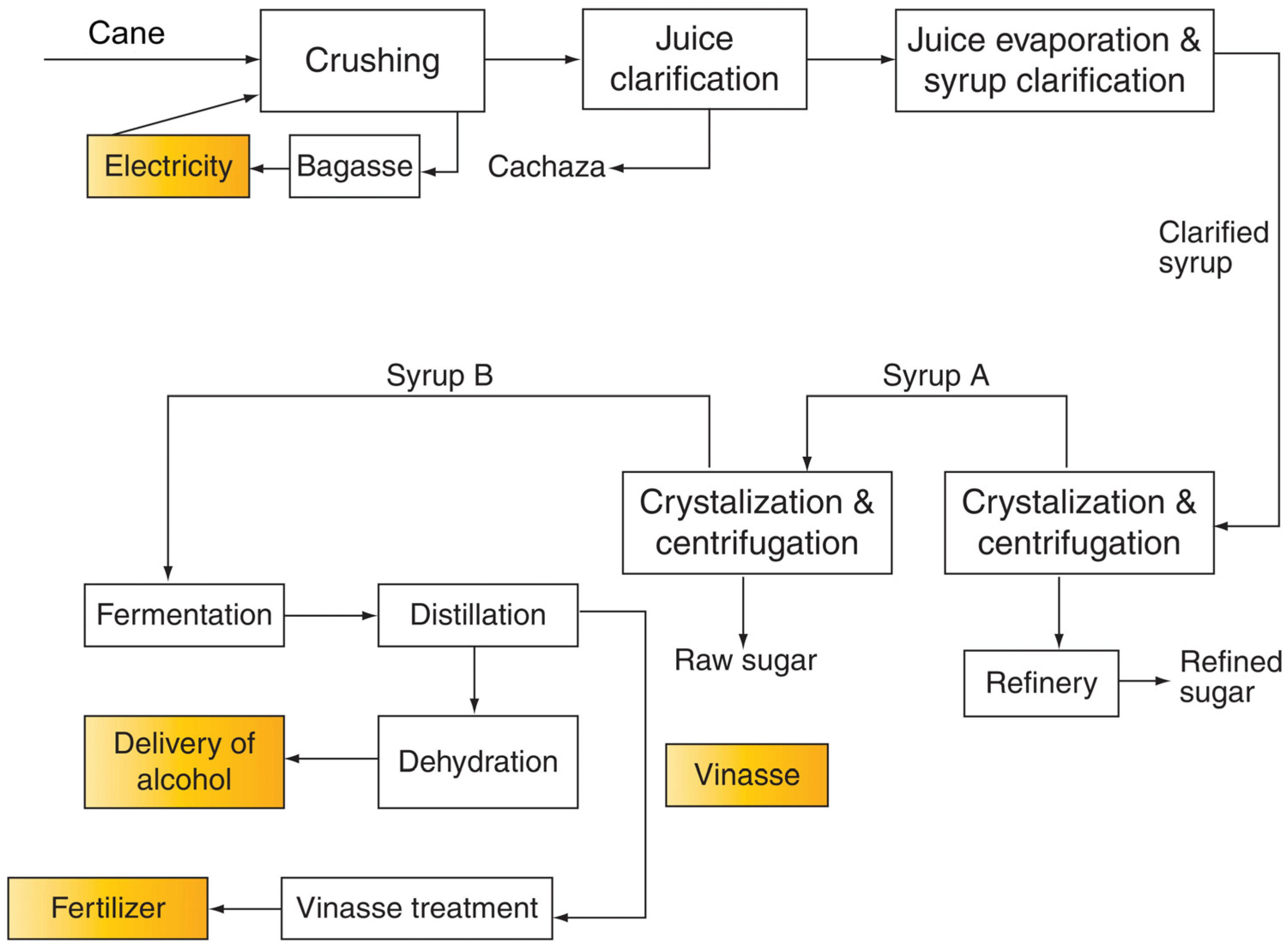
2.1. Case Study: A Colombian Sugarcane Milling Plant

The process starts in the field where the cane is partially burnt to eliminate the leaves and to facilitate the cutting. Figure 1 shows a simplified scheme of the production process [10]. Once brought to the plant, the cane is ready to undergo the preparation step, the aim of which it is to reduce the cane pieces into suitable sizes for the operation of the mills, to break sugar bearing cells, and to facilitate the sugar extraction. Preparation is a crucial step because a greater breakage of sugar-containing cells results in higher extraction of sugar and lower bagasse moisture [11]. After crossing two leveler knives, cane preparation is passed by a shredder, which is a rotor provided by hammers, then the cane is sent to two mill tandems where it is squeezed under high pressure between successive pairs or rolls. Around 66% of cane goes to Tandem 2 provided by six mills. Each mill is moved by a steam turbine and has the aim to continue cane preparation and to separate the fiber from the sucrose-containing juice. The remaining cane is milled into Tandem 1 provided with six mills and a crusher.

Figure 1. Process in a sugarcane milling plant [10].

Figure 1. Process in a sugarcane milling plant [10].

Through the mills the separated fiber forms the bagasse that has typical moisture of 50% and is sent to the boilers. Thanks to the addition of hot imbibition water, the sucrose extraction from cane reaches the 96% while 4% is lost with the bagasse. The juice is collected into tanks and lime is added. Then, the juice is heated through a series of heat exchangers. The next step is the clarification of the juice. Settled mud is produced, which undergoes a filtration process that allows the recovery of deposited sucrose. The final sludge is used as compost.

Clarified juice enters a five-effect evaporator tandem, the aim of which is to increase the brix degrees of the solution, which means to concentrate the juice. The steam extracted by the different effects (Gas) has a slightly higher temperature than the water saturation temperature at each effect pressure, because of the presence of sucrose, which implies a Boiling Point Rise. Each gas is exploited in the different steps of the process. After being concentrated, the juice is ready to produce sugar crystals. This happens through sugar boiling in vacuum pans, where low pressure and heat supply are used to create the conditions of supersaturation. Thus, sucrose crystals separate from the solution. The output of the pan is called Massecuite. It then forms crystals and a syrup called molasse. Massecuite is sent to centrifuges where crystals and molasses are divided. Crystals go to the refining process and molasses goes to the B pans where the same procedure is done. Molasses separated by B pans and B centrifuges are then sent to the distillery to produce ethanol, while B crystals are dissolved into water and recycled to the A pans, where crystals are melted and the solution undergoes the refining step, the aim of which it is to remove the remaining impurities and color of the sucrose. This is reached by another clarification with the addition of phosphoric acid and calcium saccharide, and by filtration through activated charcoal.

The solution is then ready to release its sucrose content. Another passage through vacuum pans is performed and sugar is finally delivered. B molasses from B pans are firstly fermented by the action of yeasts, which transform sucrose into ethanol and carbon dioxide, then distillated until the azeotropic point (95.6% ethanol). The azeotropic ethanol is dehydrated with molecular sieves.

The plant requires heat, electrical, and mechanical energy to fulfill the process demand. Firstly, the energy cycle was designed only to fulfill the plant requirements, since it is equipped with a wide variety of machinery. Therefore, the energy inefficiencies have been historically accepted, and eventual steam surplus are commonly released to the atmosphere. The Rankine cycle for the cogeneration of electricity, mechanical work, and heat is structured with three different pressure heads of 28.6 bar, 21.7 bar, and 2.7 bar. As shown in Figure 2, the steam is generated in three different boilers: Boiler A, B, and C. In Boiler C, the steam is generated at 28.6 bar and 410 °C, before undergoing a tempering process down to 370 °C, and only bagasse is burnt. Bagasse has a lower heating value (LHV) of 7984 kJ/kg. Boilers A and B generate superheated steam at 21.7 bar and 330 °C and burn both bagasse and coal, the latter has a LHV of 23,303 kJ/kg.

Figure 2. The cogeneration cycle in a sugarcane milling plant.

Figure 2. The cogeneration cycle in a sugarcane milling plant.

The plant is equipped with 23 turbines, operating on the two available enthalpy drops and supplying energy to different equipment. The head of 28.6 bar feeds five turbines for electrical power generation, the turbines that run the turbo-pumps of Boiler C, and the turbine of the fan of the same boiler. All the other turbines are connected to the head of 21.7 bar. There are turbines joined to the pumps and fans of Boilers A and B, turbines used to move the mills, the shredder, and the crusher. At the exit of all the turbines, steam is at the pressure of 2.7 bar, which is maintained through the addition of tempering water at saturated vapor condition. The head of 2.7 bar provides most of the steam for the heat requirement of the sugar and ethanol processes. Part of the ethanol distillery (PAC (Planta de Alcohol Carburante, which means Fuel Alcohol Plant) in Figure 2) and some equipment of the sugar plant, like the drier, are fed with steam from the head of 21.7 bar. The circuit of steam is provided by two pressure reduction stations that laminate the steam from 28.6 to 21.7 bar, and from 21.7 to 2.7 bar. Since the plant is not connected to the electrical grid, all the electrical energy produced is internally consumed.

The described process was modeled and solved in MATLAB (R2010b) in order to obtain the mass and energy balances. Many equations necessary to describe these balances are available in the literature [11,12].

2.2. Electrical Energy and Steam Requirements in the Sugar and Bioethanol Plant Production

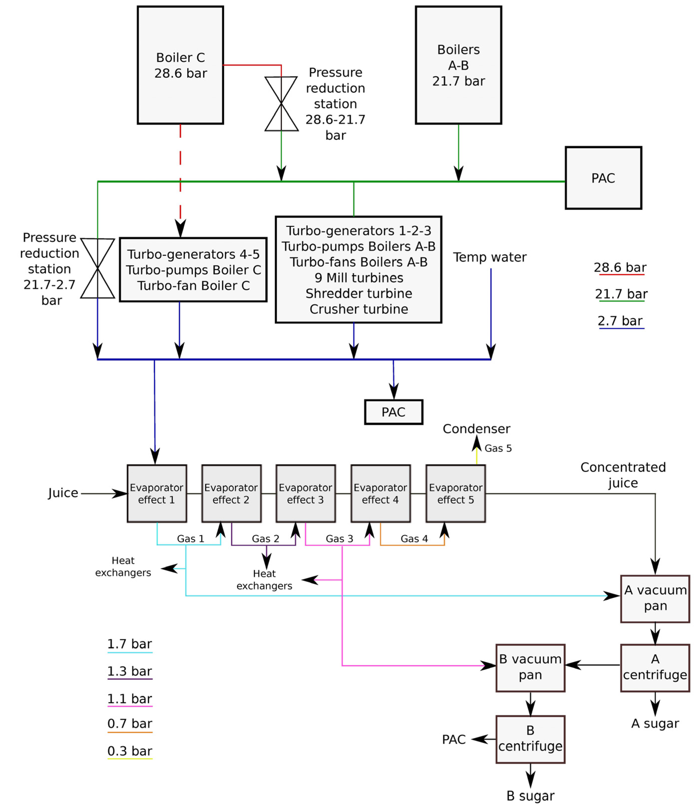
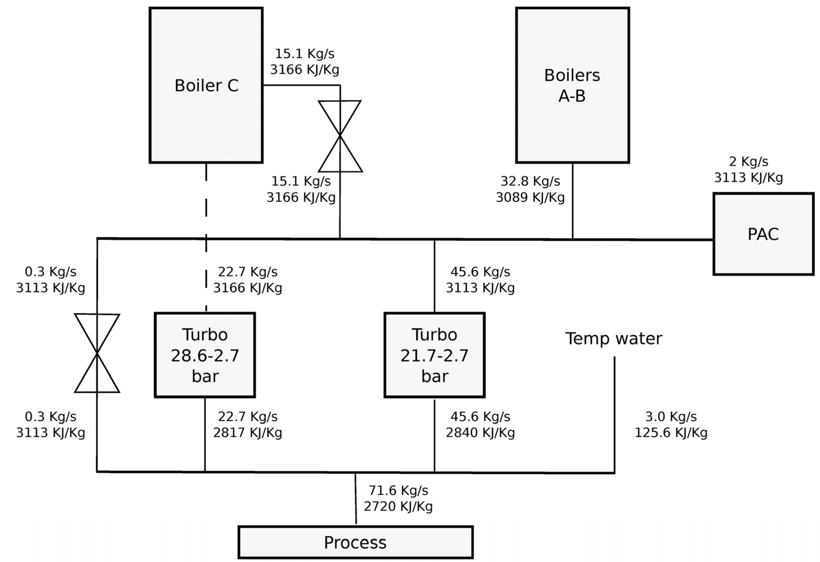
Electrical needs in the sugar plant were introduced into the model from real measurements through statistical analysis. A linear regression was performed to obtain the dependence between electrical consumption (Y, kWh/day) of the sugar plant and milling rate (mr, ton/day), and the correlation was:

Y = 6.9174 × mr + 104777 (kWh/day)

(1)

where R² = 0.756 which, according to the ISO 500001:2011 [13], is a sufficient indicator to establish the relationship. The study based on the normative outlined that 71.5% of the plant electrical energy demand was not related to the production [13]. The study showed that for the alcohol plant there was no relationship between milling rate and electrical consumption. For this reason, the electrical consumption of the PAC was a constant equal to 50,360 kWh/day. Total electrical energy consumption of the plant is the sum of the mill rate-depending part and the constant one (PAC). The electrical power requirement (P_el) is then:

(2)

The total steam requirement of the plant as a function of the milling rate is known because the steam mass rate at the outlet of boilers is measured. Equation 3 expresses the steam need (m_vap), which is translated into heat power need Q_need of the whole plant with Equation 4:

m_vap = 20.32 × mr^−0.453 ×1000 / (3600 × 2.205) (kg/s)

(3)

Q_need = 234.86 × mr + 54546 (kW)

(4)

Once again, the statistical study on the PAC steam requirement showed that it was possible to assume that there was no correlation between steam demand of the PAC and milling rate. Because of this, PAC steam consumption was considered constant (9 kg/s). The plant produces grossly 300 m³/day of ethanol.

2.3. Cogeneration

Figure 2 shows a simplified scheme of the cycle displaying the modeled blocks. With this configuration only the steam required by the process is produced and all the produced energy (electrical and mechanical) is consumed inside the plant. Then, the sugar and alcohol demands are the drivers. For a determined milling rate, heat requirements of these processes are fixed and steam mass rates are also known. This fact implies that the amount of steam required by the “PAC” and the “Process” is known. Moreover, the power requirements and the mass rates of the turbines are determined. Equation 2 provides the relationship between milling rate and electrical demand, while the mill tandem power and shredder power (P_mill, P_shred) were assumed as constant (P_mill = 12.7 (kW/tfh-mill) P_shred = 34.98 (kw/tfh)). The steam mass rates of turbo-generators, the mills’ turbines, the shredders and crushers are calculated based on the mass and energy balances. The turbines connected to turbo-pumps and the turbo-fans are related to the steam flowing to the boilers and are modeled as constant at their nominal power. With these assumptions the two blocks of the scheme that represent the turbines can be modeled.

Given the power of the turbines (P_output), the blade to shaft efficiencies η_BS, and the thermodynamic points at which they work (h_in, h_out), steam mass rates (m_vap) are calculated with Equation 5:

(5)

The tempering water block mass rate is obtained taking into account that the head of 2.7 bar is under saturated vapor conditions. This implies recursive calculation because of the possible presence of laminated steam coming from the head of 21.7 bar. Given the specific enthalpy of steam in the head of h_H2.7, total steam mass rate at turbines outlet m_VAP-T, specific enthalpy of total steam mass rate at turbines’ outlet h_out-TURB, steam mass rate crossing the 21.7 to 2.7 bar reducers m_VAP-R21, specific enthalpy of steam in the head of 21.7 bar h_H21, specific enthalpy of 2.7 bar saturated steam h_{SAT 2.7bar}, and the specific enthalpy of tempering water h_W, the following expressions were used to calculate the required mass rate of tempering water m_TW:

(6)

(7)

The blocks relative to the reduction stations are obtained by subtraction. The steam mass rate through the reducer from 21.7 to 2.7 (m_VAP-R21) bar is different from zero if the steam requirement of the head of 2.7 bar m_VAP-N2.7 is greater than the steam flowing through the blocks of the turbines (m_VAP-TURB):

m_VAP-R21 = m_VAP-N2.7 – m_VAP-TURB – m_TW (kg/s)

(8)

The reduction in steam pressure from 28.6 to 21.7 bar (m_VAP-R28) is almost constant at different milling rates because, due to its higher efficiency, Boiler C is kept at full capacity (cap_Bc) and the steam requirement of the head of 28.6 bar is almost constant too. Then, the steam flowing to this reduction station is given by the subtraction of this head requirement (m_VAP-N28) from the Boiler C capacity (Equation 9). The production on Boilers A and B (m_VAP-B-ab) then covers the other part of the 21.7 bar demand (m_VAP-N21) which is given by the requirement of the 21.7 bar turbines (m_VAP-TURB21), the steam flowing through the reduction station, and by the PAC’s requirement (m_VAP-PAC). Equations 9 to 11 provide the steam mass balance at pressure reducer at Boilers A and B, while with Equation 12 the energy balance on the 21.7 bar head is computed:

m_VAP-R28 = cap_Bc – m_VAP-N28 (kg/s)

(9)

m_VAP-N21 = m_VAP-TURB21 + m_VAP-R28 + m_VAP-PAC (kg/s)

(10)

m_VAP-B-ab = m_VAP-N21 – m_VAP-R28 (kg/s)

(11)

(12)

The following parameters were assumed to describe the Rankine cycle:

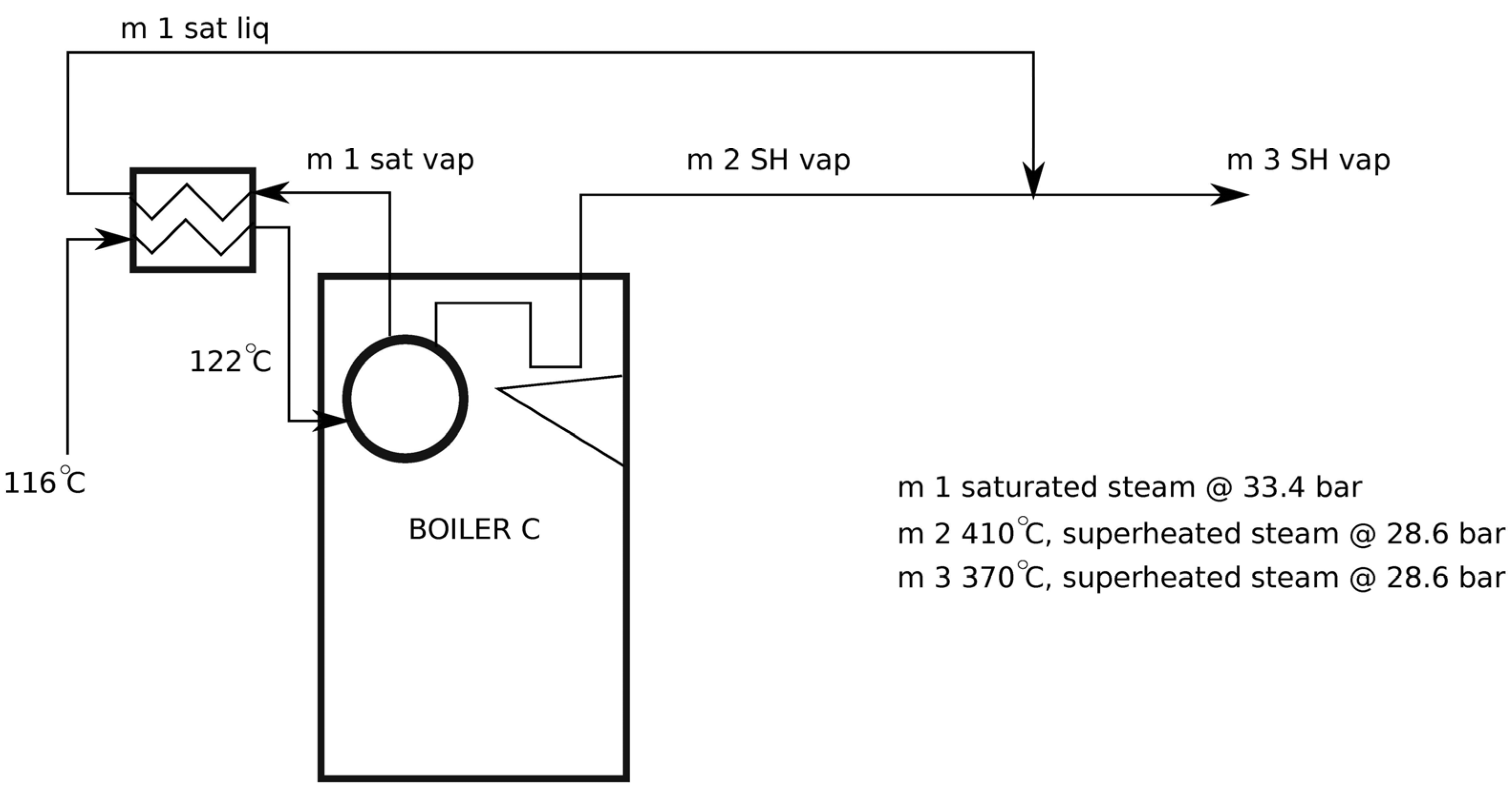
• Temperature and pressure of Boiler C: T_Bc = 410 °C; p_Bc-SH = 28.6 bar;
• Pressure of Boiler C saturated steam: p_Bc-sat = 33.6 bar;
• Temperature and pressure of Boilers A and B: T_Bab = 330 °C; p_Bab = 21.7 bar;
• Boilers efficiency: η_Bab = 0.58; η_Bc = 0.64;
• Temperature after Boiler C tempering water addition: T_Bc-TEMP = 370 °C;
• Temperature loss from boilers A and B to 21.7 bar turbines: ∆T_Bab-turb = 10 °C;
• Isentropic efficiency of the turbines: η_IS-turb = 0.60;
• Isentropic efficiency of turbines for electrical power generation 4 and 5: η_IS-TG45 = 0.68;
• Mechanical efficiency of the turbines (blades-shaft): η_B-S = 0.98;
• Electrical efficiency of the generators: η_el = 0.95;
• Turbine discharge pressure: p_VE = 2.7 bar;
• Nominal power of Turbo-fan of boilers: PVTIa = 253 kW; PVTIb = 201 kW; PVTIc = 615 kW;
• Nominal power of Turbo-generators: PTG1 = PTG2 = 1250 kW; PTG3 = 2500 kW; PTG4 = 3760 kW; PTG5 = 8510 kW.

Regarding the production of electrical energy, Turbo-generator 5 is the first used until reaching 60% of its nominal output power. If more energy is required then Turbo-generator 4 is started until reaching 50% of its nominal output power. Next, the other three turbos are switched on at full capacity, in the order of Turbo-generator 3, then 2 and at last 1.

The boiler efficiency was calculated under the nominal conditions, after addition of tempering water. It is given by the ratio between the energy content of the steam mass rate leaving the boiler at 370 °C and the energy content of the inlet fuel. This definition does not really describe the boiler performance at different conditions because it is affected by the selected value of the tempering. It is possible to calculate the efficiency of the thermal exchange inside the boiler, where water is heated until being divided into two different streams of superheated (410 °C, 28.7 bar) and saturated (33.4 bar) steam. The energy and mass balances including these two streams can be performed by knowing that their mixture will produce superheated steam at 370 °C. An accurate measurement of the steam temperatures at different loads would allow to build the efficiency curves of the boilers but it was supposed that, under different load conditions, the boiler was run with the same excess of air and that it operated with the same efficiency [14]. Therefore, it is reasonable to assume that the efficiency of the thermal exchange inside the boiler is constant. This value was calculated to be 0.6574. Figure 3 depicts the streams in Boiler C, where 33.4 bar saturated steam is firstly condensed and then mixed to 410 °C and 28.6 bar superheated steam. Knowing the inlet and outlet temperatures of feed water, the energy balance shows that more than 30% of the energy released by the condensing saturated steam is lost.

Figure 3. Scheme of Boiler C and tempering water addition.

Figure 3. Scheme of Boiler C and tempering water addition.

The indicators that have been selected to describe the performance of the cogeneration were the electrical efficiency η_el, thermal efficiency η_th, mechanical efficiency η_mech, and global efficiency of the plant η_g. By introducing the fuel heat power input of Boiler C (Q_FUEL-Bc) and of Boilers A and B (Q_FUEL-Bab), the steam mass rate produced by Boiler C (m_VAP-Bc) and by Boilers A and B (m_VAP-Bab), specific enthalpy difference of steam between outlet and inlet of Boiler C (∆h_BC) and of Boiler A and B (∆h_Bab), total heat fuel power input of the plant (Q_FUEL), useful heat power used in the process of sugar and ethanol production (Q_US), heat power used in juice heating (Q_J), effect one evaporation (Q_EVAP-EFF1), alcohol production (Q_PAC), sugar drying (Q_D), and the efficiency parameters were calculated as follows:

Q_FUEL-Bc = m_VAP-Bc × ∆h_Bc × η_Bc (kW)

(13)

Q_FUEL-Bab = m_VAP-Bab × ∆h_Bab × η_Bab (kW)

(14)

Q_FUEL = Q_FUEL-Bc + Q_FUEL-Bab (kW)

(15)

Q_US = Q_J + Q_EVAP-EFF1 + Q_PAC + Q_D (kW)

(16)

P_mech = P_mills + P_shredder + P_crusher (kW)

(17)

(18)

(19)

(20)

η_g = η_el + η_th + η_mech (kW)

(21)

3. Results and Discussion

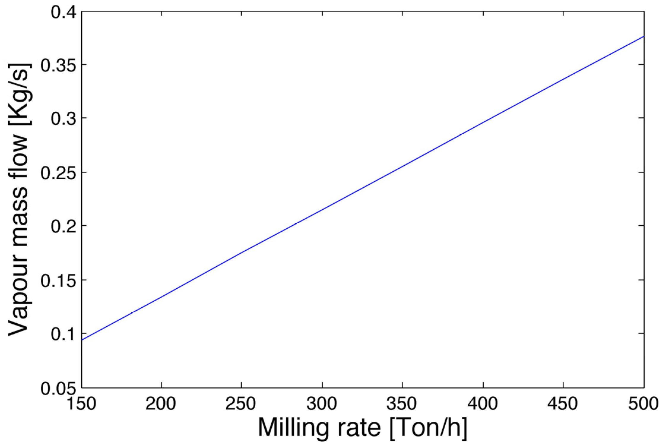
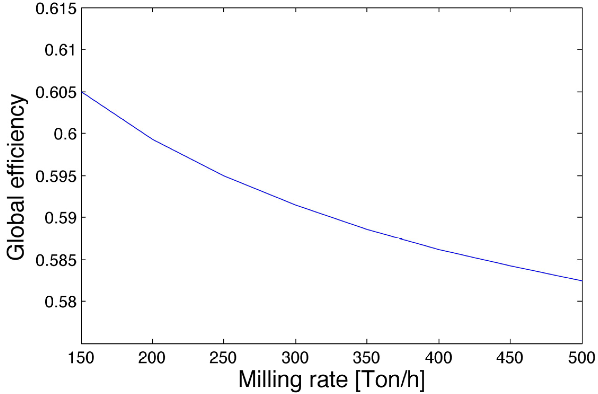
3.1. Milling Rate Dependence

Once the model was run at a specified milling rate, the mass and energy balances were calculated. Figure 4 shows that at a 430 ton/h milling rate, a fraction of total generated steam is flowing through the reduction stations (m_VAP-R28, m_VAP-R21). Under these conditions, the computed global efficiency of the plant is 58.49%. Notice the stream of 15.1 kg/s, and the one of 0.3 kg/s flowing through the 28.6 to 21.7 bar and 21.7 to 2.7 bar reduction stations, respectively. Figure 4 reports the steam mass rate and specific enthalpy in each step of the cogenerative cycle.

Figure 4. Mass and energy balances of cogeneration at 430 ton/h of cane.

Figure 4. Mass and energy balances of cogeneration at 430 ton/h of cane.

3.2. Exergy Losses

Now it is possible to compute the second principle efficiency (η_II) and the loss of energy related to critical steps. The η_II in the steady-state current condition is equal to 19.62%. Equation 22 shows how to calculate η_II, where P_el stands for electrical power, P_mech for mechanical power, Q for useful heat power, and Q_FUEL is the fuel energy input.

(22)

Energy represents the amount of useful work, which could be extracted by a system, and its definition takes into account the quality of the different forms of energy of the system and parameters to release this energy to the environment [15]. If it is of interest, energy (ε) may be expressed as:

ε = h – h_REF – T_REF × (s – s_REF) (kJ/kg)

(23)

where the subscript ref stands for reference, and s is the specific entropy. Each process is characterized by energy losses (ε_LOSS). Energy balance in a steady-state process is:

ε_in + ε_th = ε_out + P_mech + ε_LOSS (kJ/kg)

(24)

In the present study, the evaluation of energy losses in processes like pressure reductions and temperature control with tempering water has also been performed because of its importance. The pressure reductions were considered as isenthalpic, but their energy is not conserved and leads to considerable losses. Table 2 shows energy losses.

3.3. Renewable Efficiency

The “Renewable Efficiency” (η_REN) of the plant can be defined as the amount of energy produced in a renewable way with respect to the total energy required by the plant. Since bagasse represents 31% of the total cane weight, and its mean LHV (7984 kJ/kg) is known, it is possible to calculate the instantaneous bagasse flow (m_BAG), the yearly bagasse production (m_BAG-y), and the renewable efficiency, as shown in the following equations, by introducing the concepts of year equivalent hours HR_eq-y, bagasse yearly available heat power Q_BAG-y:

m_BAG= 0.31× m_c (kg/s)

(25)

(26)

(27)

Q_BAG-y = m_BAG-yx × LHV_BAG

(28)

(29)

The calculation on the year balance provided a renewable efficiency of 97.6%. This means that the plant is not energy self-sufficient; but some coal has to be introduced to the boiler. Such a value confirms that the current configuration is far from the state-of-the-art technology, which may provide η_REN higher than 100%.

Table 2. Energy losses in pressure reductions and tempering water addition at steady-state.

Process	Energy loss [%]
Boiler C tempering	3.6
28.6 to 21.7 bar reduction	3.2
21.7 to 2.7 bar reduction	26.4
2.7 bar head tempering	1.2

Table 2. Energy losses in pressure reductions and tempering water addition at steady-state.

Process	Energy loss [%]
Boiler C tempering	3.6
28.6 to 21.7 bar reduction	3.2
21.7 to 2.7 bar reduction	26.4
2.7 bar head tempering	1.2

The plant performance is related to the milling rate. The following two figures focus on the global efficiency and on the steam mass rate flowing through the 21.7 to 2.7 bar reduction station. Figure 5 shows that the steam mass rate, which undergoes this pressure reduction, increases with the milling rate. While increasing the milling rate, the heat demand of the process cannot be covered by the steam flowing through the turbines (and covering mechanical and electrical needs), and additional steam has to be processed through the 21.7 to 2.7 bar steam reduction station to guarantee the required steam mass by the process. This implies an increased loss of energy that represents a process weakness. Moreover, the increase of the steam mass rate based on the reduction raises the specific enthalpy of the 2.7 bar head. This head has to be kept in saturated steam. Then more tempering water has to be introduced into the head, causing a greater energy loss. The trend of the global efficiency is strongly affected by the steam mass rate through the reduction station, as shown in Figure 6. The selected logic for the modeling of the cogeneration implies that the steam mass rate reduced from 28.6 to 21.7 bar is constant with respect to the milling rate. Since the main part of electrical power required is not related to the production, even at very low or high milling rates the turbo-generators 4 and 5 produce the same power, because they are asked to work at a fraction of their nominal power. Moreover, as previously defined, the turbo-pump and turbo-fan of Boiler C are modeled as constants. Boiler C is working at constant full capacity at each milling rate, the steam mass rate required by the 28.6 bar turbines is constant, and then the mass flow through the 28.6 to 21.7 bar steam reduction stations remains constant.

Figure 5. Steam mass rate through the 21.7 to 2.7 bar reduction station.

Figure 5. Steam mass rate through the 21.7 to 2.7 bar reduction station.

Figure 6. Global efficiency (as defined in Equation 21) of the sugarcane plant as a function of milling rate.

Figure 6. Global efficiency (as defined in Equation 21) of the sugarcane plant as a function of milling rate.

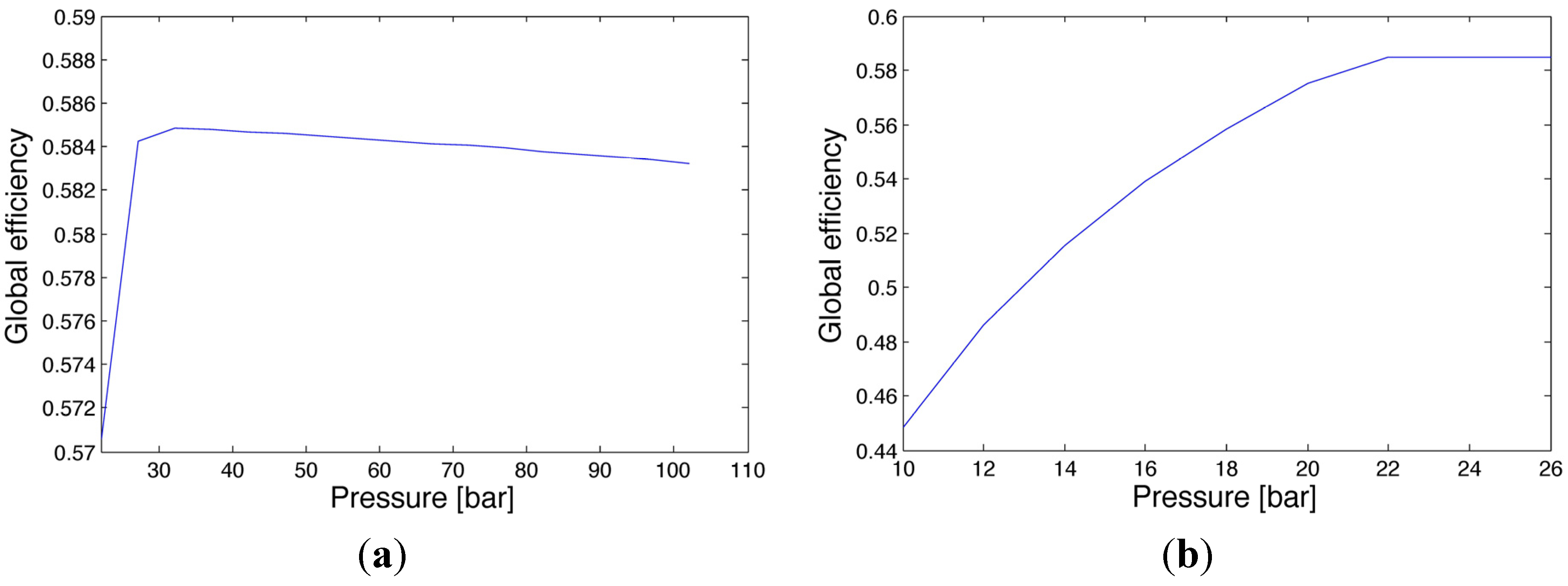
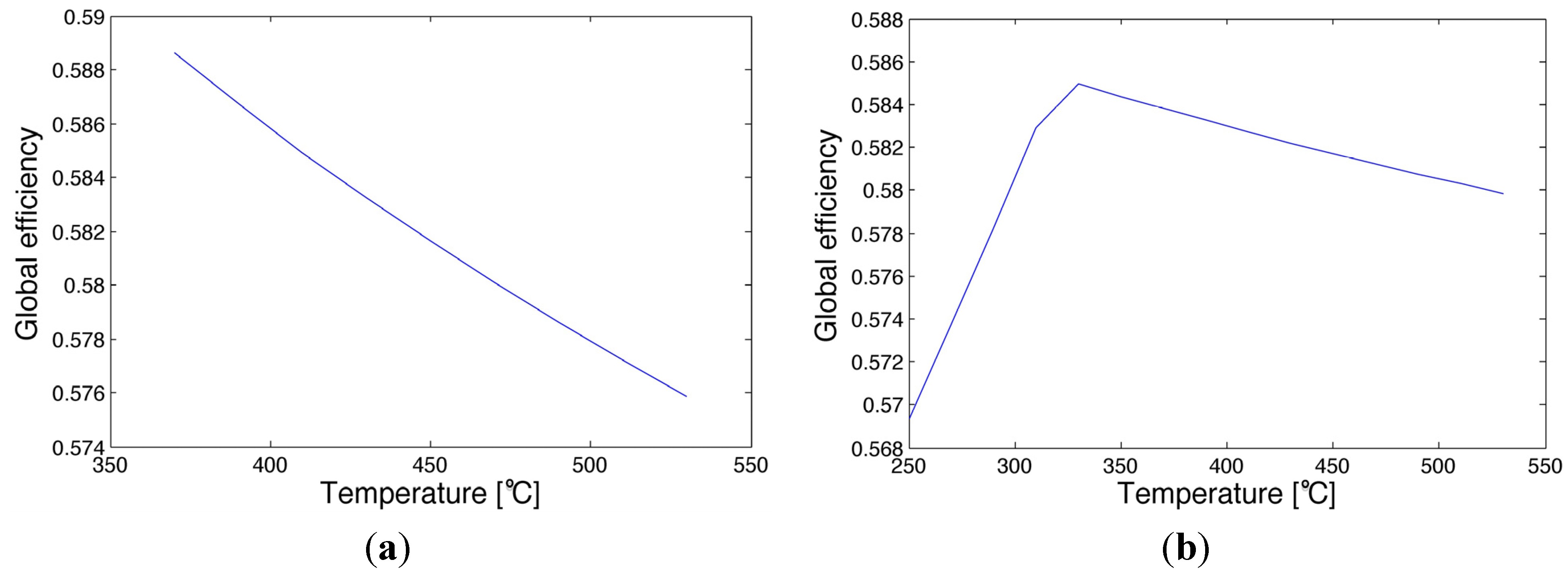
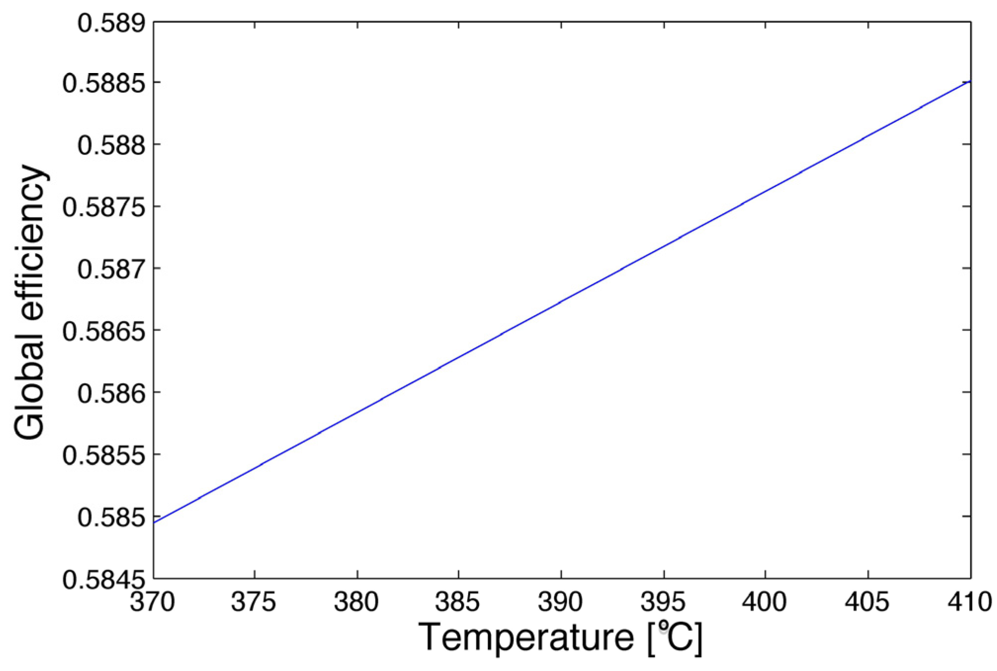
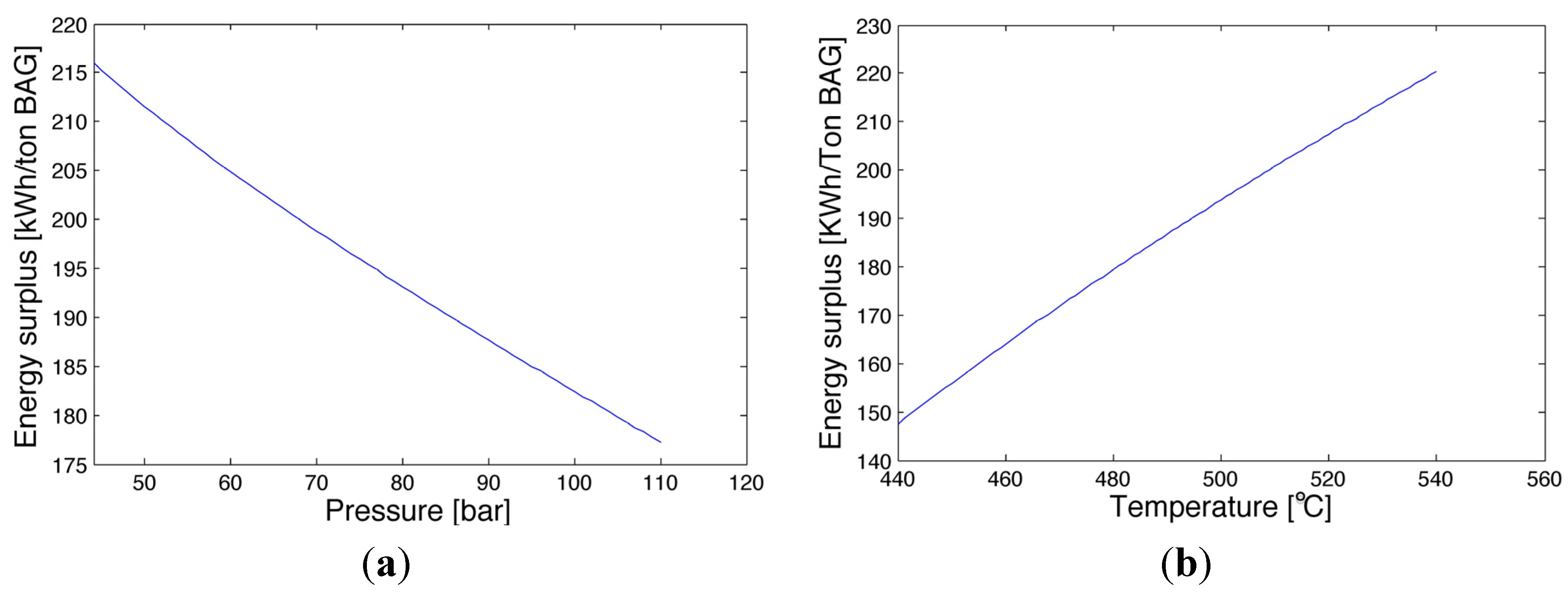
3.4. Sensitivity Analysis

Sensitivity analysis considers the effect of selected variables over considered objective functions. In this case, the objective function was η_g, and the selected variables were pressures and temperatures of boilers and tempering. The analysis was performed on the nominal plant operation. When a variable effect is studied all the others are kept constant. Figure 7a shows the effect of Boiler C outlet pressure on the η_g. Notice that an optimum is detected.

At low pressures, it appears that the global efficiency increases with pressure until reaching 20 bar (Figure 7b), when pressure reduction of the steam starts to supply the process heat requirements. From this point on the efficiency decreases. Analyzing the thermodynamic aspect of the increase of Boiler A and B pressures (for eligible values close to the nominal condition) while keeping the temperature constant implies a decrease of specific enthalpy of the 21.7 bar head. The enthalpy of the turbine outlet decreases as well, and the result is an increase of the enthalpy drop in the expansion, with a consequent decrease of steam mass rate through the 21.7 bar turbines. Consequently, the steam mass crossing the 21.7 to 2.7 bar reduction station increases, and the η_g decreases. The decrease in the pressure of Boilers A and B has the opposite effect on η_g.

Figure 7. Effect of Boilers pressure on global efficiency: (a) Boiler C; (b) Boilers A and B.

Figure 7. Effect of Boilers pressure on global efficiency: (a) Boiler C; (b) Boilers A and B.

Figure 8a shows a negative trend of η_g with the increase of inlet temperature of Boiler C with a fixed tempering temperature. The rise of the boiler internal temperature implies a mix of a high temperature steam with a lower temperature water. The bigger the temperature difference, the stronger the effect on η_g, because more saturated steam has to be condensed, thereby losing important energy content. The temperature inside the boiler does not affect the steam reduction, because this variable only involves the thermal exchange inside the boiler, but the boiler’s output conditions are controlled by the temperature at tempering output, and are then fixed. Figure 8b shows the decreasing trend of global efficiency with the temperature of Boilers A and B. If the temperature raises, the enthalpy of steam increases, the change of operation point leads to an increase of enthalpy difference across the expansion. Thus, the steam mass rate required by the 21.7 bar turbines decreases and the steam mass rate through the 21.7 to 2.7 bar reduction station increases to fulfill the requirement of the process. If the temperature is reduced from the nominal one, no steam pressure reduction is necessary and the η_g has a positive increasing trend with increasing temperature.

The tempering temperature of Boiler C has a positive impact on η_g as displayed in Figure 9. Its range is limited by the boiler’s internal temperature. The tempering is aimed at protecting the turbines from thermal stress by controlling the temperature of steam, but it represents a considerable energy loss, as shown in Table 2. Losses decrease if the tempering temperature is closer to the boiler internal temperature.

Figure 8. Effect of Boilers temperature on global efficiency. (a) Boiler C; (b) Boilers A and B.

Figure 8. Effect of Boilers temperature on global efficiency. (a) Boiler C; (b) Boilers A and B.

Figure 9. Effect of Boiler C tempering temperature on global efficiency.

Figure 9. Effect of Boiler C tempering temperature on global efficiency.

3.5. Numerical Optimization

The optimization of Rankine cycles has been widely studied [16,17]. Dias and others optimized the second-generation ethanol production [18], while other authors focused on obtaining the economical optima [19]. Here, the optimization of the η_g was carried out with an algorithm based on the Pattern Search method [20,21].

The objective function was the η_g (Equation 21), and the vector of variables was composed by pressures and temperatures of the boilers and temperature of Boiler C tempering (T_Bc.temp). In practical cases, it has to be considered that all the machines and equipment are designed with specific nominal values of temperatures and pressures. In particular, it is not allowed to change pressures at the inlet of turbines. The tempering output temperature cannot be equal to the one inside the boiler because it would lose its function to prevent variations in boiler’s temperature to affect the turbines. For these reasons, it was chosen to have a minimum gap of 10 °C.

Turbo-generators 4 and 5 accept a possible change in their inlet temperature of 5 °C, the turbo of the head of 21.7 bar can accept larger changes, because they are smaller and already operating at different temperatures, depending on the milling rate. The variables are then reduced to the only temperatures. Their bounds are given in Table 3. The temperature of the tempering has to be lower than the one inside the boiler, the outlet temperature of the turbines has to be higher than the saturation temperature at 2.7 bar (and 5 °C are added to this value as a safety margin). Moreover the maximum steam production capacity of Boilers A and B was set to 38 kg/s.

Table 3. Range of the variables for the optimization with real bounds.

Temperature	Minimum value (°C)	Maximum value (°C)
Boiler C	365	540
Boilers A and B	320	340
Boiler C tempering output	365	375

Table 3. Range of the variables for the optimization with real bounds.

Temperature	Minimum value (°C)	Maximum value (°C)
Boiler C	365	540
Boilers A and B	320	340
Boiler C tempering output	365	375

The optimization was run on a MacBook Pro (Apple Inc., Cupertino, CA, USA) machine, with a 2.7 GHz Intel Core i7 (Intel Corporation, Santa Clara, CA, USA) processor, with a 4 GB, 1333 MHzRAM memory. The results were grossly obtained after 5 h and showed that a very small increase in the global efficiency is possible. This optimal condition can be obtained by lowering the pressures of the boilers, leaving the same temperatures for Boilers A and B, decreasing the temperature of Boiler C by a couple of degrees until reaching the minimum allowed temperature difference with the stream at the outlet of tempering process. A comparison of the current and optimum case is given in Table 4. Mass and energy balances show that the optimum was obtained in correspondence with a mass rate of steam reduced from 21.7 to 2.7 bar equal to zero. The potential saving for a milling rate of 430 ton/h was calculated as 107,800 €/year.

4. Scenarios to Improve the Global Efficiency

Sugar plants are evolving into two different directions: the rise of pressure and temperature of boilers or the switch to BIGCC systems [4,6,8]. In both strategies, there is a substitution of steam driven equipment with electrical ones. The production of electrical energy with bigger turbines allows better energy conversion and simplification. Then, the possibility to upgrade and repower the case study plant is considered. The final aim is to produce an electrical energy surplus to be sold to the national electrical grid. Steam consumption reduction, substitution of steam driven machines, and new possible layouts for repowering were evaluated.

Table 4. Current and optimal case comparison considering real bounds.

Milling rate: 430 Ton/h	p boiler C (bar)	T boiler C (°C)	p boilers A, B (bar)	T boilers A, B (°C)	Toutlet tempering boiler C (°C)	Global efficiency
Current case	28.6	410	21.7	330	370	0.5849
Optimal case	28.6	380	21.7	320	370	0.5880

Table 4. Current and optimal case comparison considering real bounds.

Milling rate: 430 Ton/h	p boiler C (bar)	T boiler C (°C)	p boilers A, B (bar)	T boilers A, B (°C)	Toutlet tempering boiler C (°C)	Global efficiency
Current case	28.6	410	21.7	330	370	0.5849
Optimal case	28.6	380	21.7	320	370	0.5880

It is estimated that the process steam demand, at a milling rate of 430 ton/h, could be reduced by 36.7 kg per ton of cane through the change of some heat exchangers and dividing the juice heating process into more stages. According to this estimation, 4.4 kg/s of steam could be saved, corresponding to 11.3 thermal MW. With this configuration the second principle efficiency may increase by 2% and the plant may reach 101% of Renewable Efficiency. With such an improvement in the production process, the cogeneration becomes the weak part of the process. This means that the turbines require a higher amount of steam than the production process, and this affects the performance indicators.

Two repowering layouts were proposed based on the current available technology. The first repowering option is the simplest one: besides the Boiler C scheme, a new Superheated Rankine Cycle is set up, with extraction at 2.7 bar, regeneration, and condensing pressure. The second repowering option is similar to the first one but has a slightly more complex new cycle, which is provided by reheating at medium pressure. The starting point is the calculation of available fuel heat power. Being interested in the optimization at a milling rate of 430 ton/h, the result is that the plant can work for the same equivalent hours per year and the instantaneous availability of fuel energy is 295 MW.

The capacity of the new boiler depends heavily on its pressure and temperatures, which determine the amount of steam that can be produced with the available fuel heat power. The logic of the new scheme is to fully exploit the heat capacity of the bagasse, by satisfying the energy requirement of the sugar and ethanol plants, and by producing a surplus of electrical energy. Boiler C may produce less steam the power of which is limited to 12 MW, and obtained with a mass rate of 36.6 kg/s, which is able to cover 80% of the process heat demand. The new boiler and cycle being characterized by higher efficiency, Boiler C could be chosen to be operated at 50% of nominal capacity. Under these conditions, Boiler C would cover 41% of heat process demand.

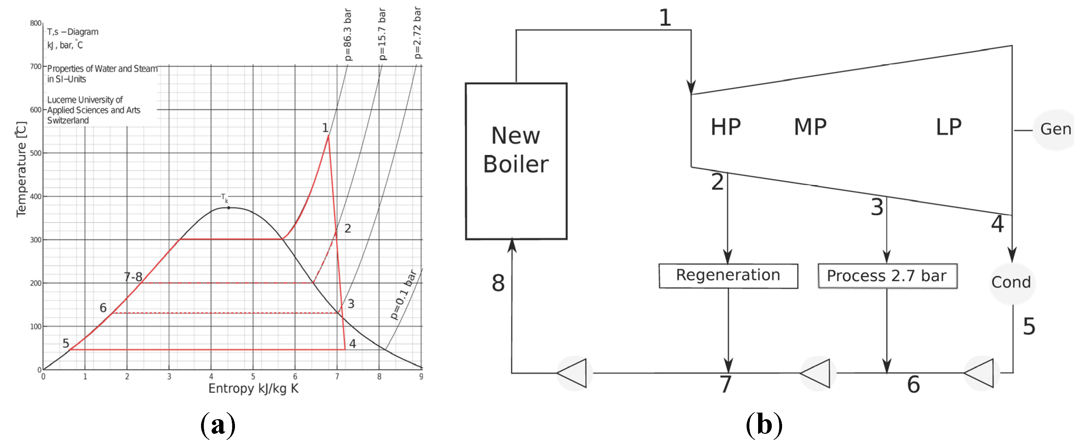
4.1. Option 1 Repowering

The T-s diagram of the new cycle shown in Figure 10 immediately remarks the limit of the new cycle. Once the bleeding is fixed at 2.7 bar to be slightly supersaturated to avoid condensation in the head before the sugar process, Point 3 of the extraction follows in the chart. A strong limitation on the increase of pressure and temperature of the boiler is introduced because of the thermodynamic limit of the isentropic efficiency. The isentropic efficiency is represented by the slope of the expansion line, Point 1 to Point 4 in Figure 10, and it cannot be too steep.

As the characteristics of the bottoming cycle of 28.6 bar should not be changed, the variables to be studied in order to optimize the objective function are pressure and temperature of the new cycle, which were chosen to be commercial boilers, pressure of regeneration, and steam mass rate of regeneration that influence the inlet temperature of boiler. The minimum capacity of the boiler was determined for each couple of pressure and temperature, while the condensing pressure was chosen to be 0.1 bar, with the water available at around 30 °C and considering a condenser split temperature of 15 °C. Figure 10 also depicts the layout of the new Option 1 cycle.

Figure 10. (a) T-s diagram of Repowering Option 1; (b) Process layout of Repowering Option 1.

Figure 10. (a) T-s diagram of Repowering Option 1; (b) Process layout of Repowering Option 1.

1: Turbine inlet; 2: Regeneration bleeding; 3: Process bleeding; 4: Turbine outlet; 5: Condenser outlet; 6: Process condensed water; 7: Addition of regeneration vapor; 8: Pump and boiler’s inlet.

The model is similar to the current case, with the difference that the turbine is characterized by different mass rates in high, medium, and low pressures. Moreover, being Boiler C running at minimum capacity, the steam it produces provides 41% of the process steam demand. In this way, the new cycle satisfies the remaining 59% of steam requirement. The objective function is given by the electrical energy surplus that can be obtained by each ton of bagasse. Being P_el-surplus the total plant electrical power surplus, the energy index E_index is expressed in Equation 31:

(30)

The sensitivity analysis of boiler pressure in Figure 11 shows the negative trend assumed by the energy surplus when the pressure rises. The reason of this is found in what was previously remarked to be a strong constraint of the model. Forcing the temperature at 2.7 bar bleeding to be 135 °C (5 °C of super saturation), the effect of raising the pressure implies a change in the slope of the expansion on the T-s diagram. From a thermodynamic point of view, it means a decrease in the isentropic efficiency of the turbine. The available enthalpy drop between inlet and outlet of the turbine is less exploited and a decrease in efficiency and work output occurs. Figure 11 also presents the sensitivity analysis of the boiler temperature. The energy surplus behaves in the opposite way than with pressure. It increases with temperature because the rise of temperature implies a higher isentropic efficiency of the expansion, and then a higher work output and cycle efficiency. For both of these variables, not all the values are possible, because the isentropic efficiency of the expansion has to assume reasonable values (<0.9), so temperature cannot freely rise until material limits and pressure decrease too much.

The optimization to find efficiency in repowering Option 1 has to take into account several limits, on both top and bottom cycles. In particular, the temperature of the feed water after the mix with regeneration steam T₇, has to be lower than the saturation temperature, and hence, a security margin of 3 °C was chosen. The steam fraction x₄ at the end of the expansion has to be higher than 0.87 to avoid excessive condensation inside the turbine, and the flow rates in the turbines have to be higher than 0. For each possible pressure and temperature combination of the boilers, pressure and mass rate of regeneration are optimized and verified to satisfy all the technical and thermodynamic constraints. The results are shown in Table 5. In Table 5, the minimum new boiler capacity and the power required by the new turbine are reported as well. These values are necessary for the design of the new equipment.

Figure 11. Effect of new cycle boiler’s pressure and temperature on energy surplus index in Option 1 repowering. (a) Pressure; (b) Temperature.

Figure 11. Effect of new cycle boiler’s pressure and temperature on energy surplus index in Option 1 repowering. (a) Pressure; (b) Temperature.

Table 5. Results of optimization for repowering with Option 1 at different boiler conditions.

Boiler P (bar)	Boiler T (°C)	Boiler capacity (kg/s)	Boiler Inlet T (°C)	p reg (bar)	mvap reg (kg/s)	P turbine top (MW)	ηis	Psurplus (MW)	ηII plant	Surplus (kWh/tonBAG)
45.1	440	57.4	176	9.8	7.9	37.2	0.871	23.9	0.2371	179.2
64.7	485	56.7	187	12.5	8.6	39.9	0.863	26.5	0.2459	198.7
66.7	510	55.9	192	13.7	8.7	42.2	0.9000	28.7	0.2534	215.4
85.3	515	56.5	196	14.8	9.2	41.5	0.8468	27.9	0.2507	209.4
86.3	515	56.8	199	15.8	9.5	41.5	0.8440	27.8	0.2505	208.9
86.3	540	55.5	199	15.7	9.1	43.8	0.8858	30.2	0.2584	226.4
87.3	515	57.1	202	16.7	9.8	41.4	0.8411	27.8	0.2503	208.5
104	540	56.8	208	19.0	10.2	42.9	0.8415	29.2	0.2551	219.0
106.9	540	57.1	210	19.7	10.4	42.8	0.8350	29.0	0.2545	217.8
108.9	540	56.9	208	18.8	10.2	42.7	0.8306	28.9	0.2542	217.0

Table 5. Results of optimization for repowering with Option 1 at different boiler conditions.

Boiler P (bar)	Boiler T (°C)	Boiler capacity (kg/s)	Boiler Inlet T (°C)	p reg (bar)	mvap reg (kg/s)	P turbine top (MW)	ηis	Psurplus (MW)	ηII plant	Surplus (kWh/tonBAG)
45.1	440	57.4	176	9.8	7.9	37.2	0.871	23.9	0.2371	179.2
64.7	485	56.7	187	12.5	8.6	39.9	0.863	26.5	0.2459	198.7
66.7	510	55.9	192	13.7	8.7	42.2	0.9000	28.7	0.2534	215.4
85.3	515	56.5	196	14.8	9.2	41.5	0.8468	27.9	0.2507	209.4
86.3	515	56.8	199	15.8	9.5	41.5	0.8440	27.8	0.2505	208.9
86.3	540	55.5	199	15.7	9.1	43.8	0.8858	30.2	0.2584	226.4
87.3	515	57.1	202	16.7	9.8	41.4	0.8411	27.8	0.2503	208.5
104	540	56.8	208	19.0	10.2	42.9	0.8415	29.2	0.2551	219.0
106.9	540	57.1	210	19.7	10.4	42.8	0.8350	29.0	0.2545	217.8
108.9	540	56.9	208	18.8	10.2	42.7	0.8306	28.9	0.2542	217.0

The difference in the cash flow respective to the current situation has to be evaluated. The cash flow represents the sum of all the revenues and costs that the process implies. The new revenues are given by selling electrical energy and by savings related to the coal that is replaced. Some coal may be bought to guarantee flame stabilities in the boilers but it would not affect the cash flow. The saving related to the coal is mostly related to the decrease of process steam demand, thus it is not considered in this work. It is estimated that the electrical energy could be potentially sold at a price of 0.048 €/kWh. The best results are given by the boiler with 86.3 bar and 540 °C, with a boiler inlet temperature of 199 °C obtained with a regeneration bleeding of 9.1 kg/s, at 15.6 bar of pressure. This configuration would give a year cash flow of 8,665,500 €/year.

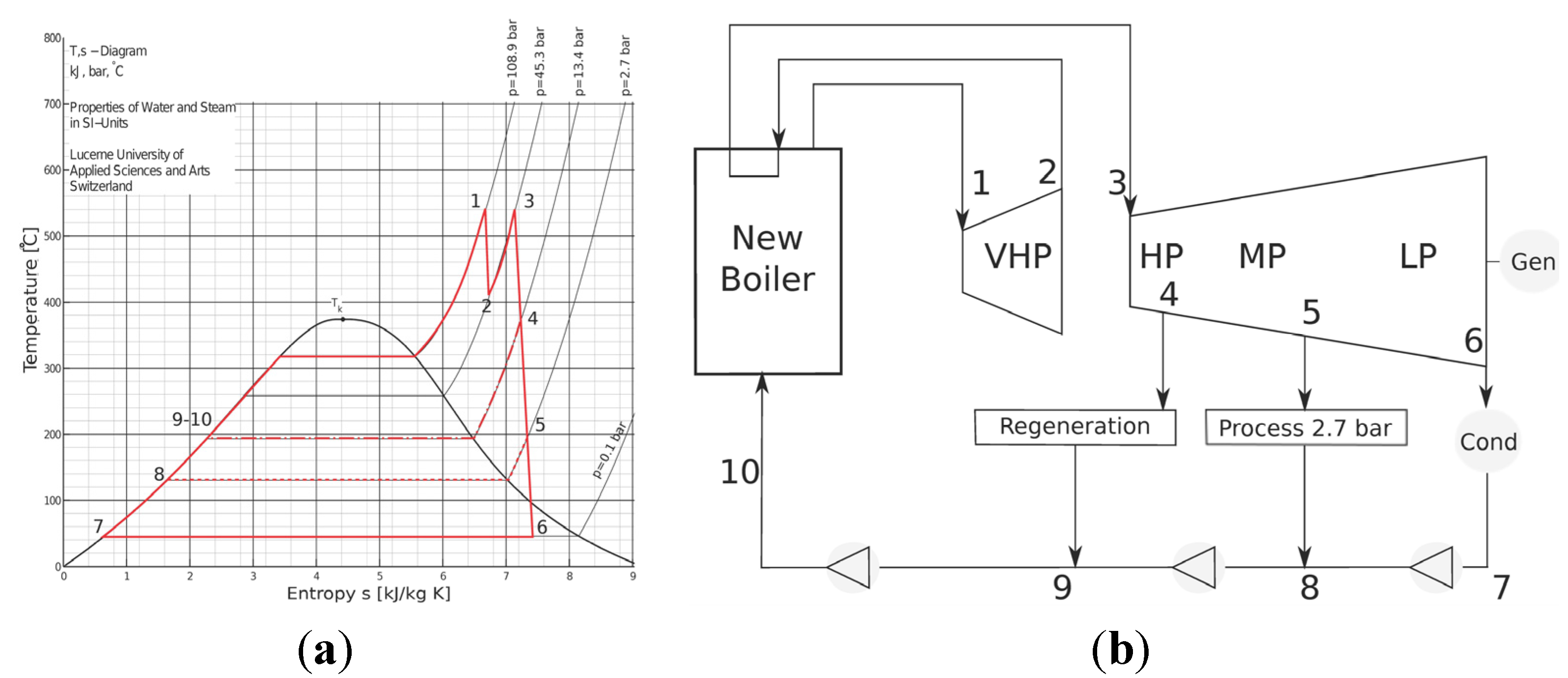
4.2. Option 2 Repowering

In Option 2, the expansion is divided into two blocks of turbines because of the reheating. For the first block, an isentropic efficiency of 88% is assumed, while the one of the second turbine is a variable, left free to float until a maximum value of 90%. In this case, the turbine outlet temperature is not fixed, but it is a parameter computed by the model, whereby the fact that it has to be at least 5 °C superheated is considered as a constraint. The available fuel power is fixed, the plant is designed in a way that, in steady state conditions, all the produced bagasse is burnt in the boilers and the old Boiler 7 is run at minimum capacity. The variables characterizing the systems are pressure and temperature of the boiler (to be chosen among the commercial available devices), isentropic efficiency of second turbine, pressure of reheating, and pressure and steam mass rate of regeneration.

Figure 12 shows the T-s diagram for repowering Option 2 with the respective layout. For the sensitivity analysis, boiler pressure and temperature are assigned the optimum value of the previous case, reheating pressure is set to 45 bar, regeneration at 16 bar with 2 kg/s of bled steam and the isentropic efficiency of the second part of expansion is fixed at 80%. The choice of these values may influence the results of the sensitivity analysis, so they are chosen far from their upper and lower limits. Once all other variables are fixed, and assuming that the fuel power input is given, the pressure of the boiler has a positive influence on the energy surplus, as shown in Figure 13, because, on a T-s diagram, it corresponds to increasing the area under the thermodynamic cycle by turning away the lines of heating.

The temperature of the boiler, pressure and steam mass rate of regeneration, have identical behaviors to the repowering Option 1. The optimization of the second layout has the same range, and similar constraints to previous proposal, with the only addition of a linear constraint forcing reheating pressure to be higher than the regeneration one. Optimization results are shown in Table 6. The higher the couple boiler pressure and temperature, the better results can be obtained. Maximum energy surplus index is obtained with a boiler of 108.9 bar and 540 °C, which could give 251.9 kWh per each ton of bagasse. The optimal configuration is obtained with a reheating pressure of 43.8 bar, regeneration bleeding of 8 kg/s at 15.3 bar. In this case, with no point of the expansion fixed, the optimization follows the typical behavior of Rankine cycles, which can reach the highest performances with the highest possible pressure and temperature at the expansion inlet. The cash flow related to the selling of optimal energy surplus is 9,639,600 €/year and is greater than Repowering Option 1.

4.3. Economic Analysis of Repowering Options

Both repowering options were evaluated in terms of the feasibility of the investment. With the new configuration proposal being a very first step of the design process, a fifth class cost estimation was carried out aimed at establishing the order of magnitude of the investment [22]. The total fixed capital cost is the sum of direct and indirect costs. Direct costs included purchased equipment, purchased equipment installation, instrumentation and controls, piping and electrical (installed) buildings, yard improvements, service facilities, and land. Indirect costs included engineering and supervision, construction expenses, contractor’s fee and contingency [23]. The equipment to be bought included a boiler, turbine, generator, condenser and electrical motors for the mills, pumps and fans. To estimate the investment of the purchased equipment, the procedure consisted of two steps based on the knowledge of the costs of a device similar to the one to be bought [23,24].

Table 6. Results of optimization for repowering Option 2 with diverse boiler conditions.

Boiler P (bar)	Boiler T (°C)	Boiler capacity (kg/s)	Boiler Inlet T (°C)	p reheat (bar)	p reg (bar)	mvap reg (kg/s)	P turbine top (MW)	ηis	P surplus (MW)	ηII plant	Surplus (kWh/tonBAG)
45.1	440	51.9	163	22.2	6.3	5.7	39.2	0.9	25.9	0.2439	194.3
64.7	485	52.1	181	35.2	11.5	6.9	42.3	0.9	28.9	0.2540	216.8
66.7	510	49.8	176	30.9	8.4	6.1	43.3	0.9	29.9	0.2574	224.3
85.3	515	49.0	179	32.1	10.2	6.1	44.9	0.9	31.4	0.2625	235.6
86.3	515	50.9	190	40.5	11.8	7.3	45.1	0.9	31.6	0.2631	236.9
86.3	540	47.5	177	30.6	12.0	5.5	45.3	0.9	31.7	0.2637	238.1
87.3	515	52.3	221	32.9	22.1	9.3	45.0	0.9	31.5	0.2627	236.1
104.0	540	51.3	218	41.7	21.5	8.9	46.8	0.9	33.1	0.2683	248.5
106.9	540	52.6	226	47.8	24.3	9.8	46.9	0.9	33.2	0.2687	249.5
108.9	540	50.3	204	43.8	15.3	8.0	47.3	0.9	33.6	0.2699	251.9

Table 6. Results of optimization for repowering Option 2 with diverse boiler conditions.

Boiler P (bar)	Boiler T (°C)	Boiler capacity (kg/s)	Boiler Inlet T (°C)	p reheat (bar)	p reg (bar)	mvap reg (kg/s)	P turbine top (MW)	ηis	P surplus (MW)	ηII plant	Surplus (kWh/tonBAG)
45.1	440	51.9	163	22.2	6.3	5.7	39.2	0.9	25.9	0.2439	194.3
64.7	485	52.1	181	35.2	11.5	6.9	42.3	0.9	28.9	0.2540	216.8
66.7	510	49.8	176	30.9	8.4	6.1	43.3	0.9	29.9	0.2574	224.3
85.3	515	49.0	179	32.1	10.2	6.1	44.9	0.9	31.4	0.2625	235.6
86.3	515	50.9	190	40.5	11.8	7.3	45.1	0.9	31.6	0.2631	236.9
86.3	540	47.5	177	30.6	12.0	5.5	45.3	0.9	31.7	0.2637	238.1
87.3	515	52.3	221	32.9	22.1	9.3	45.0	0.9	31.5	0.2627	236.1
104.0	540	51.3	218	41.7	21.5	8.9	46.8	0.9	33.1	0.2683	248.5
106.9	540	52.6	226	47.8	24.3	9.8	46.9	0.9	33.2	0.2687	249.5
108.9	540	50.3	204	43.8	15.3	8.0	47.3	0.9	33.6	0.2699	251.9

Figure 12. (a) T-s diagram of Option 2 Repowering; (b) Layout of Option 2 Repowering.

Figure 12. (a) T-s diagram of Option 2 Repowering; (b) Layout of Option 2 Repowering.

1: VHP turbine inlet; 2: VHP turbine outlet; 3: Reheating outlet; 4: Regeneration bleeding; 5: Process bleeding; 6: LP turbine outlet; 7: Condenser outlet; 8: Condensed water; 9: Addition of regeneration vapor; 10: Pump and boiler’s inlet.

Figure 13. Effect of new cycle boiler’s pressure on energy surplus index.

Figure 13. Effect of new cycle boiler’s pressure on energy surplus index.

The first step is aimed to obtain the cost of a new device by relating its size or capacity to the known one with an exponential rule. The obtained cost is then scaled on the dimension of new equipment, but it is still related to the year in which reference price is considered. The second step updates this value to the current year by the use of indexes based on the inflation rate. In this work CEPCI (Chemical Engineering Plant Cost Index) indexes were used, updated to 2013. Selected reference sizes for new equipment cost evaluation were consulted in the literature [24], with the only exception of the boiler. The literature [24] indicates capacity (ton/h of produced steam) as a reference unit, but the presence of reheating (which implies another passage of steam in the boiler, but just in its super-heater part) complicates the usage of this reference. For this reason, fuel power input is selected. Concerning the condenser, it is sized with the LMTD method. It is as a first approach. Cooling water flow rate m_w of 600 L/s and global heat exchange coefficient U equal to 2550 W/m²·K are considered. The total purchased equipment of Option 1 and Option 2 cost 18.91 and 18.92 million Euro, respectively. Peters and Timmerhaus estimate that the cost of purchased equipment represents 15%–40% of total fixed capital cost [23]. Considering 27.5% as an average value, the investment for Options 1 and 2 are 68.78 and 68.87 million Euro, respectively.

Both the options present a net present value (NPV) higher than zero at the selected horizon. Option 1 predicts 54.38 million Euro 20 year-NPV, while Option 2 gives 68.13 million Euro. This result means that, with a given discount rate, the investment is feasible. The payback time (PBT) is 10 years for the first option, and 9 years for the second option. Half of the horizon time will be required to return the investment, while the positive cash flow rates of the other half represents profit for the company. With the same horizon, the two Internal Rates of Return (IRR) result to be 11.0% and 12.7%, respectively. Table 7 compares the most important data and indexes related to the optima solutions of both repowering alternatives.

Table 7. Economical comparison of repowering alternatives.

Variable	Option 1	Option 2
Investment (€)	18,914,782	18,940,182
Plant surplus energy index (kWh/tonBAG)	226.4	251.9
Electrical energy sell revenue (€/year)	8,665,500	9,639,600
20 years NPV (€)	54,376,553	68,128,494
PBT (year)	10	9
IRR (%)	11.0	12.7

Table 7. Economical comparison of repowering alternatives.

Variable	Option 1	Option 2
Investment (€)	18,914,782	18,940,182
Plant surplus energy index (kWh/tonBAG)	226.4	251.9
Electrical energy sell revenue (€/year)	8,665,500	9,639,600
20 years NPV (€)	54,376,553	68,128,494
PBT (year)	10	9
IRR (%)	11.0	12.7

5. Conclusion

A complete energy efficiency assessment for a big Colombian sugarcane mill was developed. The analysis of the current configuration showed some critical points in the energy efficiency, corresponding to the addition of tempering water in Boiler C and to the reduction of steam pressure. The strongest negative effect was given by the steam mass rate through a reduction station, which was necessary when the steam demand of the turbines was required to guarantee the mechanical and electrical power. The model outlines that the current process of the plant is far from the state-of-the-art technology, as is the case for many sugarcane plants in developed countries. Sugarcane mills should be able to extract a convenient energy surplus from the combustion of bagasse. However, the analyzed sugarcane mill plant covers only 97% of its own energy needs. Nevertheless, due to the way in which the plant was originally designed, the sensitivity analysis of the main variables and the numerical optimization confirm that the boilers are already working close to their optimal conditions.

The results suggest the need to involve a new cogenerative cycle to be coupled with steam reduction phases. By substituting old boilers with a new one, two different Rankine cycles were proposed to satisfy the electrical and thermal energy requirements of the plant and to produce a convenient electrical energy surplus, which could be sold in the national electricity grid. The first proposal was a normal condensing with extraction cycle, while the second proposal was a reheating cycle. The optimal first configuration allows the whole plant to reach 25.8% second principle efficiency. Better results in terms of efficiency and energy surplus may be obtained with the reheating cycle, whose second principle efficiency is 27.0%. Further studies on the analyzed sugar mill should consider the substitution of all boilers, this would imply a higher investment, but also would guarantee higher efficiencies. A more advanced study considering the switch to the supercritical Rankine cycle or to the BIGCC layout should also be done.

References

1. O’Sullivan, A.; Sheffrin, S. Economics: Principle and Tools, 2nd ed.; Prentice Hall: New Saddle River, NJ, USA, 2003. [Google Scholar]
2. International Energy Agency. World Energy Outlook 2011. Available online: http://www.iea.org/ (accessed on 28 August 2013).
3. Committee on Biobased Industrial Products, National Research Council. Biobased Industrial Products: Research and Commercialization Priorities; National Academic Press: Washington, DC, USA, 2000; p. 74. [Google Scholar]
4. Khatiwada, D.; Seabra, J.; Silveira, S.; Walter, A. Power generation from sugarcane biomass—A complementary option to hydroelectricity in Nepal and Brazil. Energy 2012, 48, 241–254. [Google Scholar] [CrossRef]
5. Purohit, P.; Michaelowa, A. CDM potential of bagasse cogeneration in India. Energy Policy 2007, 35, 4779–4798. [Google Scholar]
6. Coordination BNDES and CGEE. Sugarcane-based bioethanol, Energy for sustainable development. Available online: http://www.sugarcanebioethanol.org/ (accessed on 2 September 2013).
7. Deshmukh, R.; Jacobson, A.; Chamberlin, C.; Kammen, D. Thermal gasification or direct combustion? Comparison of advanced cogeneration systems in the sugarcane industry. Biomass Bioenergy 2013, 55, 163–174. [Google Scholar] [CrossRef]
8. Pellegrini, L.F.; de Oliveira Jùnior, S.; Burbano, J.C. Supercritical steam cycles and biomass integrated gasification combined cycles for sugarcane mills. Energy 2013, 35, 1172–1180. [Google Scholar]
9. Dias, M.O.S.; Junqueira, T.L.; Cavalett, O.; Cunha, M.P.; Jesus, C.D.F.; Mantelatto, P.E.; Rossell, C.E.V.; Filho, R.M.; Bonomi, A. Cogeneration in integrated first and second generation ethanol from sugarcane. Chem. Eng. Res. Des. 2013, 91, 1411–1417. [Google Scholar] [CrossRef]
10. Toasa, J. Colombia: A New Ethanol Producer on the Rise? United States Department of Agriculture Economic Research Service: Washington, DC, USA, 2009. [Google Scholar]
11. Rein, P. Cane Sugar Engineering, 1st ed.; Verlag Dr. Albert Bartens KG: Berlin, Germany, 2007. [Google Scholar]
12. Hugot, E. Handbook of Cane Sugar Engineering, 3rd ed.; Elsevier: New York, NY, USA, 1986. [Google Scholar]
13. International Organization for Standardization. Energy Management Systems–Requirements with Guidance for Use; ISO 50001:2011; BSI Group: London, UK, 2011. [Google Scholar]
14. Rinaldi, F.; Najafi, B. Temperature measurement in WTE boilers using suction pyrometers. Sensors 2013, 13, 15633–15655. [Google Scholar] [CrossRef] [Green Version]
15. Paz, D.; Cardenas, C.J. Evaluación exergética de propuestas de disminución de consumo de vapor en usinas azucareras. Rev. Ind. Agríc. Tucumán 2005, 82, 1–8. (In Spanish) [Google Scholar]
16. Dincer, I.; Al-Muslim, H. Thermodynamic analysis of reheat cycle steam power plants. Int. J. Energy Res. 2001, 25, 727–739. [Google Scholar] [CrossRef]
17. El-Emam, R.S.; Dincer, I. Energy and exergoeconomic analyses optimization of geothermal organic Rankine cycle. Appl. Therm. Eng. 2013, 59, 435–444. [Google Scholar] [CrossRef]
18. Dias, M.O.S.; Junqueira, T.L.; Jesus, C.D.F.; Rossell, C.E.V.; Filho, R.M.; Bonomi, A. Improving second generation ethanol production though optimization of first generation production process from sugarcane. Energy 2012, 43, 246–252. [Google Scholar] [CrossRef]
19. Furlan, F.F.; Borba Costa, C.B.; de Castro Fonseca, G.; de Pelegrini Soares, R.; Resende Secchi, A.; Goncales da Cruz, A.J.; de Campos Giordano, R. Assessing the production of first and second generation bioethanol from sugarcane through the integration of global optimization and process detailed modeling. Comput. Chem. Eng. 2012, 43, 1–9. [Google Scholar] [CrossRef]
20. Hooke, R.; Jeeves, T.A. Direct search solution of numerical and statistical problems. J. ACM 1961, 8, 212–229. [Google Scholar] [CrossRef]
21. The Mathworks Inc. Genetic Algorithm and Direct Search Toolbox for Use with Matlab User’s Guide. Available online: http://www.mathworks.com (accessed on 13 February 2014).
22. Dysert, L.R. Sharpen your cost estimating skills. Cost Eng. 2003, 45, 22–30. [Google Scholar]
23. Peters, M.; Timmerhaus, K.D. Plant Design and Economics for Chemical Engineers, 3rd ed.; McGraw Hill: New York, NY, USA, 1980. [Google Scholar]
24. Coker, A.K. Ludwig’s Applied Process Design for Chemical and Petrochemical Plants, 4th ed.; Elsevier: Burlington, MA, USA, 2007. [Google Scholar]