
Simulation of Forestland Dynamics in a Typical Deforestation and Afforestation Area under Climate Scenarios


Abstract
:1. Introduction
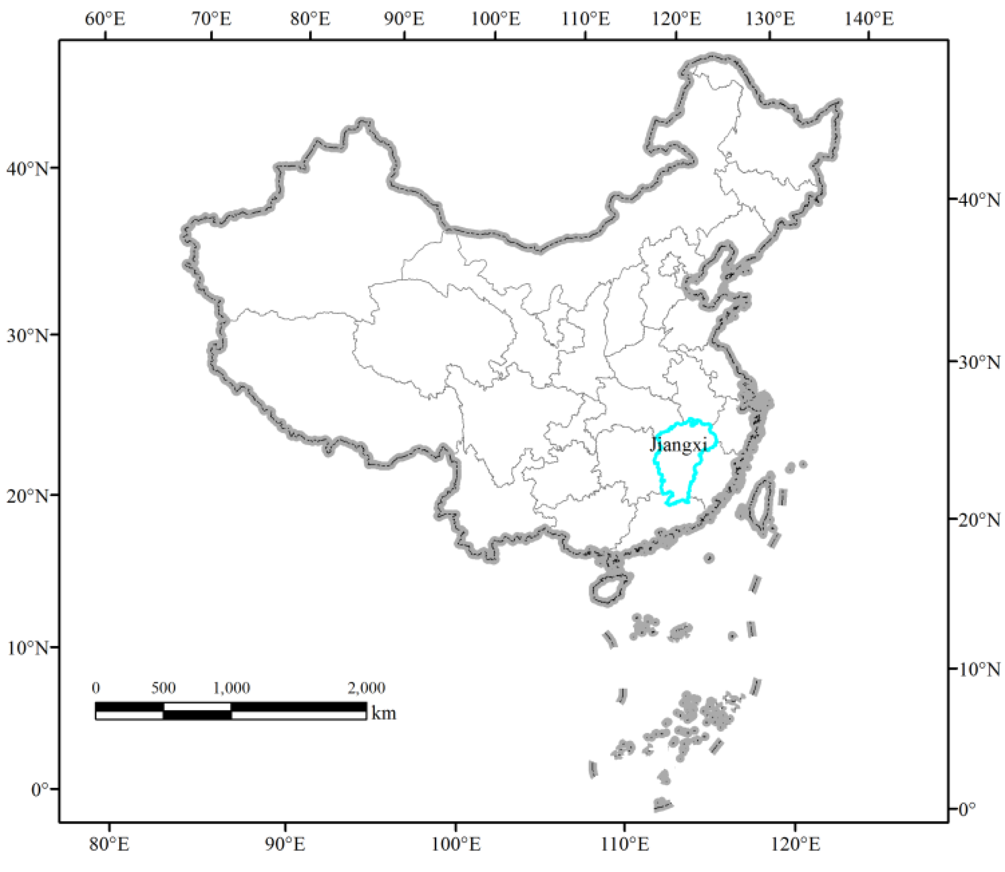
2. Study Area

3. Data and Methodology
3.1. Data Sources

| Equation | Meaning | Variables | Unit |
|---|---|---|---|
| (1) and (2) | Population density | Popden | person/km2 |
| (3) | Population | Pop | Person |
| (2) and (3) | Agricultural population, one-period lag term | Agrpop | Person |
| (1) and (2) | GDP | ln(gdp) | Million yuan |
| GDP in non-agricultural industry | ln(nagr_gdp) | Million yuan | |
| (1) and (3) | elevation | ln(dem) | m |
| (1) | Quadratic term of elevation | (ln(dem))2 | m |
| (3) | Slope | ln(slope) | Degree |
| (3) | Quadratic term of slope | (ln(slope))2 | Degree |
| (1) and (3) | Soil organic matter | ln(organic) | - |
| (1)–(3) | Precipitation | ln(pa) | mm |
| (1) and (2) | Quadratic term of precipitation | (ln(pa))2 | mm |
| (1)–(3) | Air temperature | ln(ta) | Degree |
| (1) and (2) | Quadratic term of air temperature | (ln(ta))2 | Degree |
| (1) and (3) | Distance to provincial capital | ln(d2pvcp) | km |
| (1) | Distance to port | ln(d2port) | km |
| (1)–(3) | Distance to the nearest road | ln(d2road) | km |
| (1) and (3) | Road density | ln(road_den) | km/km2 |
| Forestland | ln(Y) | km2 | |
| (1)–(3) | Forestry production | ln(fe_prod) | Million Yuan |
| (1)–(3) | Forestry output value | ln(fe_gdp) | Million Yuan |
| (3) | Whether the county is poor | Poverty | - |
| (1) and (3) | Whether the county is the major grain producing area | Grain | - |
| (1) | Whether the county is involved in the Stated-owned Forest Farms and Nursery System | Mng | - |
| (2) | Area of other land converted to forest land | ln(wother20) | km2 |
| (3) | Area of forest land converted to other land | ln(lw20other) | km2 |
| (2) | Whether the county has implemented Grain for Green | Tghl | - |
| (1)–(3) | Forestry coverage rate | Y | % |
| (2) and (3) | Quadratic term of forestry coverage rate | (Y)2 |
3.2. Methodology
3.2.1. Driving Mechanism Method
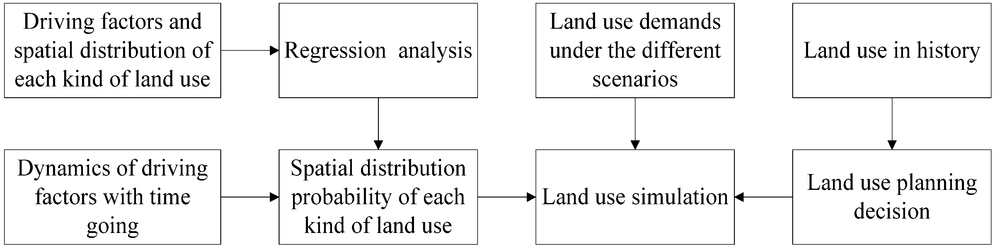
3.2.2. Conversion of Land Use and its Effects (CLUE) Model

3.2.3. Scenario Design
3.2.4. Model for Energy Supply Strategy Alternatives and their General Environmental Impact (MESSAGE) Climate Scenario

3.2.5. Asia-Pacific Integrated Model (AIM) Climate Scenario
4. Driving Mechanisms of the Deforestation and Afforestation Processes
4.1. Driving Mechanism for Density Variation of Forestland
| Y: Density Variation of Forestland | |||||||
|---|---|---|---|---|---|---|---|
| X | Equation (1) | Equation (2) | Equation (3) | Equation (4) | Equation (5) | Equation (6) | Equation (7) |
| ln(popden) | −0.427 (8.53) *** | −0.335 (6.72) *** | −0.132 (3.84) *** | −0.131 (3.81) *** | −0.113 (3.35) *** | −0.165 (4.65) *** | −0.151 (4.16) *** |
| ln(gdp_t1) | 0.069 (1.70) * | 0.039 (0.98) | −0.032 (1.31) | −0.032 (1.34) | −0.039 (1.64) | −0.031 (1.25) | −0.041 (1.51) |
| ln(fe_prod_t1) | - | 0.172 (4.59) *** | 0.033 (1.40) | 0.034 (1.44) | 0.026 (1.08) | 0.009 (0.41) | 0.019 (0.68) |
| ln(fe_gdp_t1) | - | −0.026 (0.65) | 0.002 (0.09) | 0.001 (0.05) | 0.002 (0.06) | 0.002 (0.08) | −0.026 (0.67) |
| ln(dem) | - | - | 3.325 (9.65) *** | 3.237 (9.11) *** | 2.620 (6.51) *** | 2.008 (4.69) *** | 2.073 (4.83) *** |
| Quadratic term of ln(dem) | - | - | −0.298 (9.74) *** | −0.292 (9.33) *** | −0.244 (6.99) *** | −0.201 (5.32) *** | −0.206 (5.45) *** |
| ln(slope) | - | - | 0.169 (2.25) ** | 0.185 (2.41) ** | 0.376 (3.86) *** | 0.485 (5.07) *** | 0.488 (5.08) *** |
| ln(organic) | - | - | - | 0.158 (1.00) | 0.013 (0.08) | −0.064 (0.42) | −0.052 (0.34) |
| ln(pa) | - | - | - | - | 61.772 (1.14) | 107.324 (1.95) * | 98.469 (1.79) * |
| Quadratic term of ln(pa) | - | - | - | - | −4.083 (1.12) | −7.164 (1.92) * | −6.578 (1.76) * |
| ln(ta) | - | - | - | - | 646.107 (2.29) ** | 634.687 (2.20) ** | 697.959 (2.41) ** |
| Quadratic term of ln(ta) | - | - | - | - | −6.393 (2.23) ** | −6.433 (2.19) ** | −7.097 (2.40) ** |
| ln(road_den) | - | - | - | - | - | −0.009 (0.71) | −0.009 (0.65) |
| ln(d2pvcp) | - | - | - | - | - | 0.132 (2.40) ** | 0.140 (2.52) ** |
| ln(d2road) | - | - | - | - | - | 0.196 (3.75) *** | 0.192 (3.66) *** |
| Grain | - | - | - | - | - | - | 0.072 (1.74) * |
| Mng | - | - | - | - | - | - | 0.062 (0.87) |
| Constant | 10.171 (17.59) *** | 9.803 (15.38) *** | −1.058 (1.10) | −1.006 (1.04) | −3,844.751 (2.39) ** | −3,946.200 (2.39) ** | −4,265.844 (2.56) ** |
| R2 | 0.24 | 0.32 | 0.75 | 0.76 | 0.77 | 0.80 | 0.80 |
4.1.1. Influence of Human Activities
4.1.2. Influence of Forestry Economy
4.1.3. Influence of the Natural Environment
4.1.4. Influence of Location and Transportation
4.1.5. Influence of National Policies
4.2. Driving Mechanisms of the Afforestation Process
4.2.1. Influence of Population Size
| Y: Area of other land converted to forestland | |||||
|---|---|---|---|---|---|
| X | Equation (1) | Equation (2) | Equation (3) | Equation (4) | Equation (5) |
| ln(popden) | −0.876 (17.84) *** | −0.841 (17.25) *** | −0.828 (16.81) *** | −0.817 (16.49) *** | −0.786 (16.63) *** |
| ln(agrpop) | 0.686 (13.16) *** | 0.692 (15.92) *** | 0.670 (15.03) *** | 0.664 (14.87) *** | 0.694 (16.26) *** |
| ln(gdp) | −0.138 (2.77) *** | −0.185 (4.41) *** | −0.191 (4.67) *** | −0.185 (4.54) *** | −0.117 (2.89) *** |
| ln(fe_prod_t1) | - | 0.023 (0.73) | 0.051 (1.59) | 0.046 (1.39) | 0.072 (0.28) |
| ln(fe_gdp_t1) | - | 0.088 (2.77) *** | 0.094 (3.07) *** | 0.091 (2.96) *** | 0.154 (4.89) *** |
| ln(Y) | - | 2.565 (8.40) *** | 2.390 (8.04) *** | 2.319 (7.67) *** | 2.277 (7.94) *** |
| Quadratic term of ln(Y) | - | −0.151 (7.10) *** | −0.139 (6.75) *** | −0.133 (6.29) *** | −0.130 (6.47) *** |
| ln(ta) | - | - | −1,640.635 (4.57) *** | −1,669.297 (4.40) *** | −1,577.328 (4.38) *** |
| Quadratic term of ln(ta) | - | - | 16.660 (4.56) *** | 16.953 (4.39) *** | 16.019 (4.37) *** |
| ln(pa) | - | - | - | 130.855 (1.81) * | 140.178 (2.04) ** |
| Quadratic term of ln(pa) | - | - | - | −8.854 (1.81) * | −9.478 (2.04) ** |
| Tghl | - | - | - | - | 0.285 (5.43) *** |
| Constant | −4.032 (7.27) *** | −14.473 (11.90) *** | 9,154.924 (4.56) *** | 8,831.888 (4.12) *** | 8,283.760 (4.07) *** |
| R2 | 0.69 | 0.78 | 0.79 | 0.80 | 0.82 |
4.2.2. Influence of Social Economy
4.2.3. Influence of Climate
4.2.4. Influence of National Policy
4.3. Driving Mechanism of the Deforestation Process
4.3.1. Influence of Population Size
4.3.2. Influence of Social Economy
| Y: Area of Forestland Converted to Other Land | |||||||
|---|---|---|---|---|---|---|---|
| X | Equation (1) | Equation (2) | Equation (3) | Equation (4) | Equation (5) | Equation (6) | Equation (7) |
| ln(pop) | −1.731 (6.24) *** | −1.673 (6.83) *** | −1.544 (6.24) *** | −1.542 (6.22) *** | −1.470 (5.93) *** | −1.147 (4.88) *** | −1.004 (4.19) *** |
| ln(agrpop) | 2.039 (9.64) *** | 2.045 (10.94) *** | 1.972 (10.48) *** | 1.966 (10.43) *** | 1.937 (10.32) *** | 1.445 (7.59) *** | 1.318 (6.75) *** |
| ln(nagr_gdp) | 0.112 (1.47) | 0.212 (3.16) *** | 0.173 (2.55) ** | 0.174 (2.56) ** | 0.168 (2.49) ** | 0.193 (3.15) *** | 0.161 (2.58) ** |
| ln(fe_prod_t1) | - | 0.068 (1.60) | 0.081 (1.89) * | 0.081 (1.87) * | 0.116 (2.58) ** | 0.125 (2.92) *** | 0.104 (2.40) ** |
| ln(fe_gdp_t1) | - | −0.146 (3.30) *** | −0.133 (3.03) *** | −0.132 (2.99) *** | −0.144 (3.26) *** | −0.150 (3.75) *** | −0.136 (3.39) *** |
| ln(y) | - | −1.253 (3.28) *** | −0.535 (1.08) | −0.520 (1.05) | −0.745 (1.48) | −1.285 (2.78) *** | −1.261 (2.75) *** |
| Quadratic term of ln(y) | - | −0.042 (1.61) | 0.004 (0.11) | 0.005 (0.15) | −0.007 (0.20) | −0.031 (0.94) | −0.031 (0.97) |
| ln(dem) | - | - | −0.334 (2.42)** | −0.317 (2.26)** | −0.242 (1.70)* | −0.095 (0.67) | −0.098 (0.69) |
| ln(slope) | - | - | 0.361 (2.70) *** | 0.349 (2.59) ** | 0.178 (1.18) | −0.044 (0.31) | −0.005 (0.03) |
| ln(organic) | - | - | - | −0.197 (0.69) | −0.129 (0.44) | 0.293 (1.08) | 0.361 (1.33) |
| ln(pa) | - | - | - | - | 0.139 (0.27) | −0.79 1(1.65) | −1.156 (2.33) ** |
| ln(ta) | - | - | - | - | −34.518 (2.44)** | −8.509 (0.56) | −10.391 (0.68) |
| ln(road_den) | - | - | - | - | - | 0.081 (3.49) *** | 0.080 (3.50) *** |
| ln(d2pvcp) | - | - | - | - | - | −0.115 (1.21) | −0.038 (0.38) |
| ln(d2road) | - | - | - | - | - | −0.519 (5.82) *** | −0.546 (6.14) *** |
| Grain | - | - | - | - | - | - | 0.137 (1.95) * |
| Poverty | - | - | - | - | - | - | −0.105 (1.46) |
| Constant | 0.660 (0.68) | −7.123 (4.51) *** | −3.553 (1.63) | −3.363 (1.53) | 189.461 (2.36) ** | 45.800 (0.53) | 58.774 (0.68) |
| R2 | 0.42 | 0.61 | 0.63 | 0.63 | 0.64 | 0.71 | 0.72 |
4.3.3. Influence of Topographic Conditions
4.3.4. Influence of Location and Transportation
4.3.5. Influence of National Policy
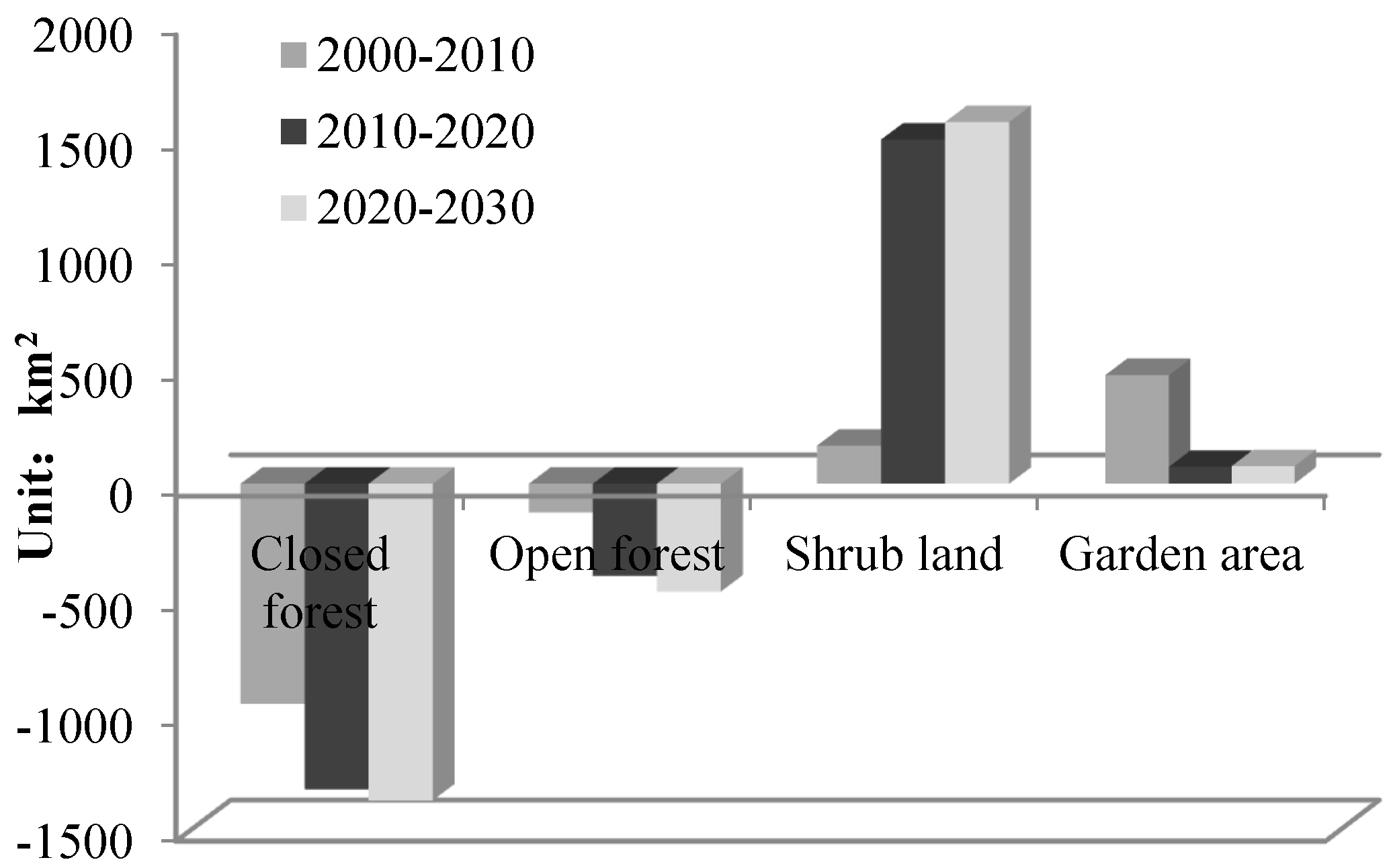
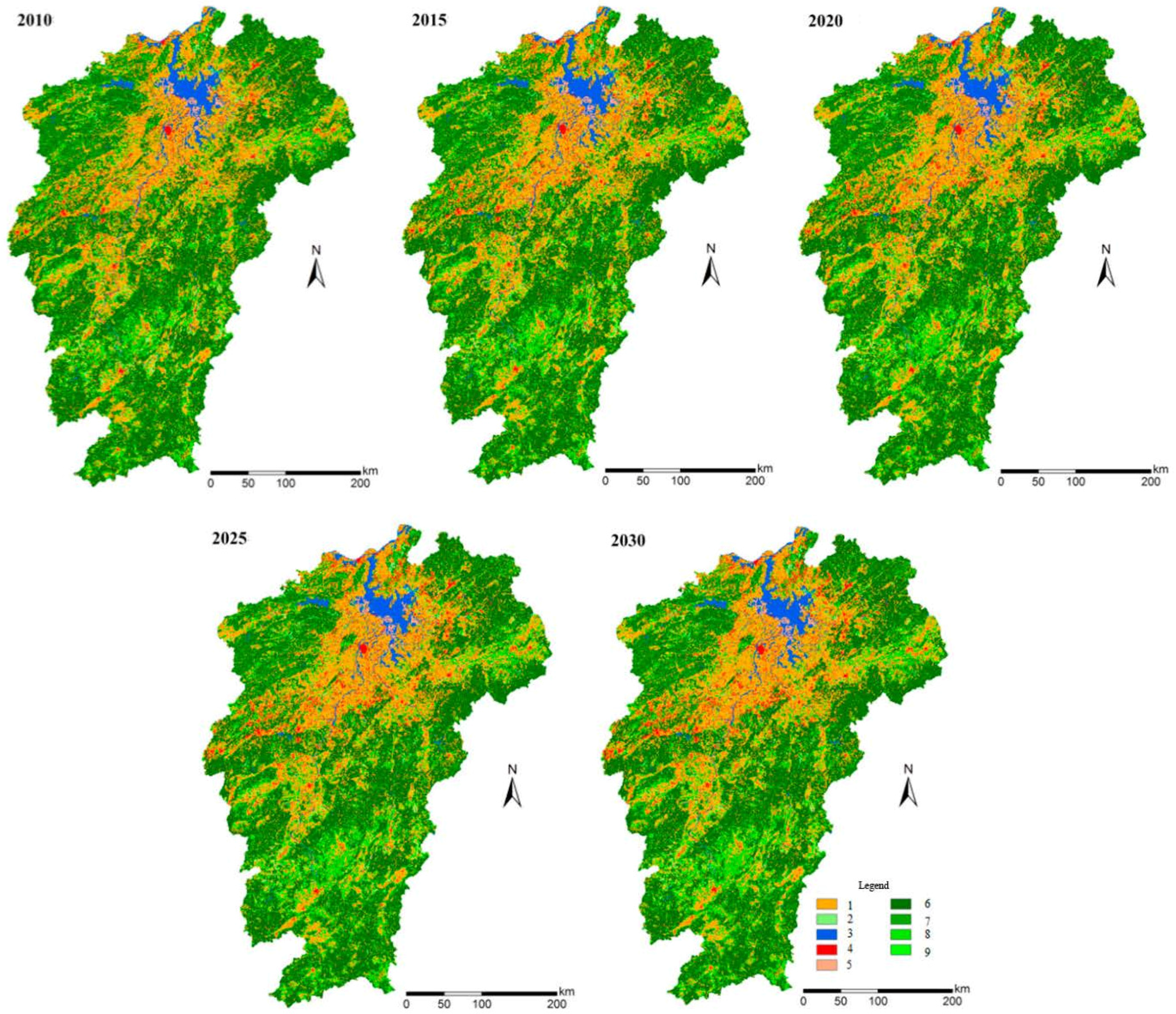
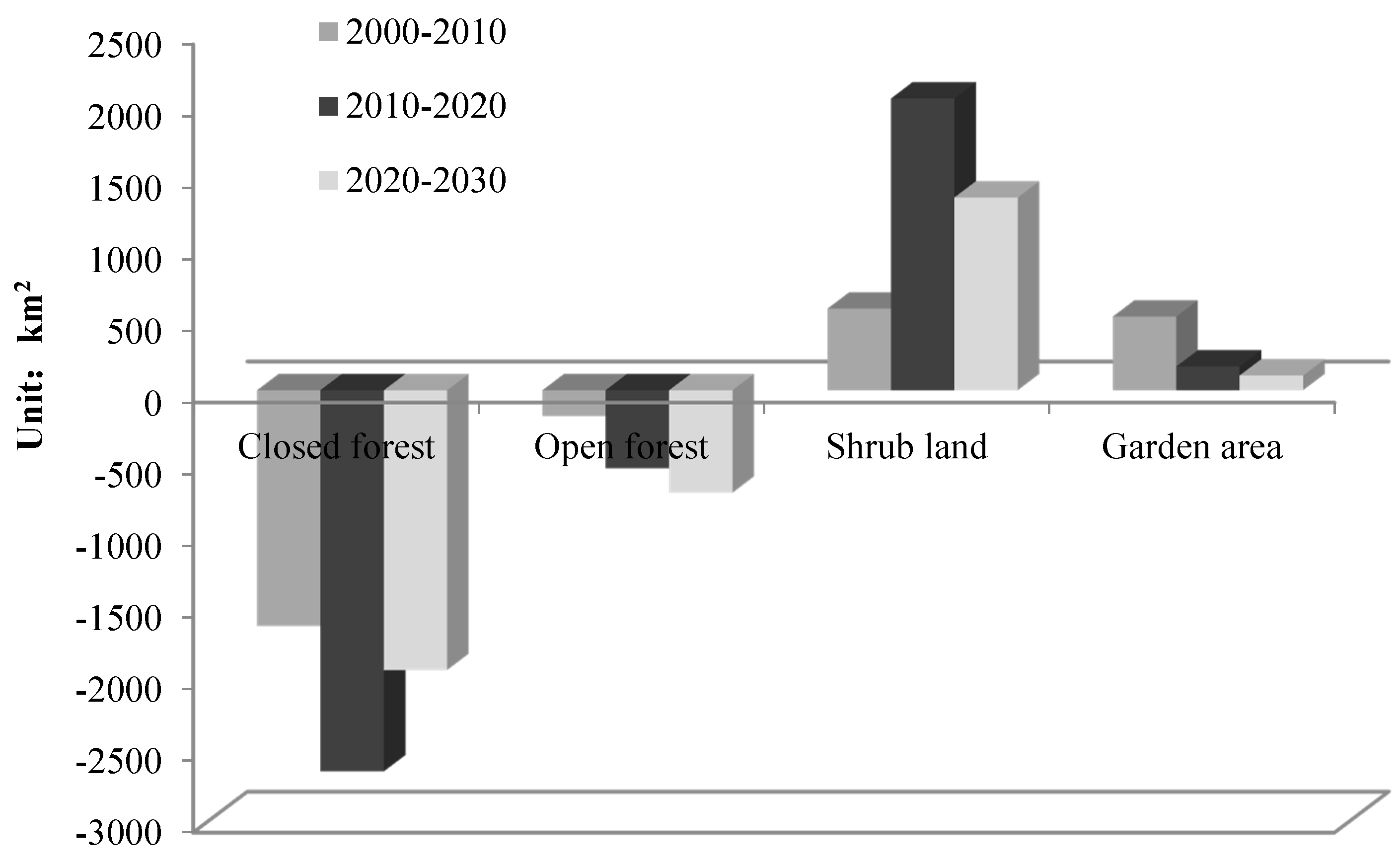
5. Simulation of the Deforestation and Afforestation Processes
5.1. Validation of Simulation Results

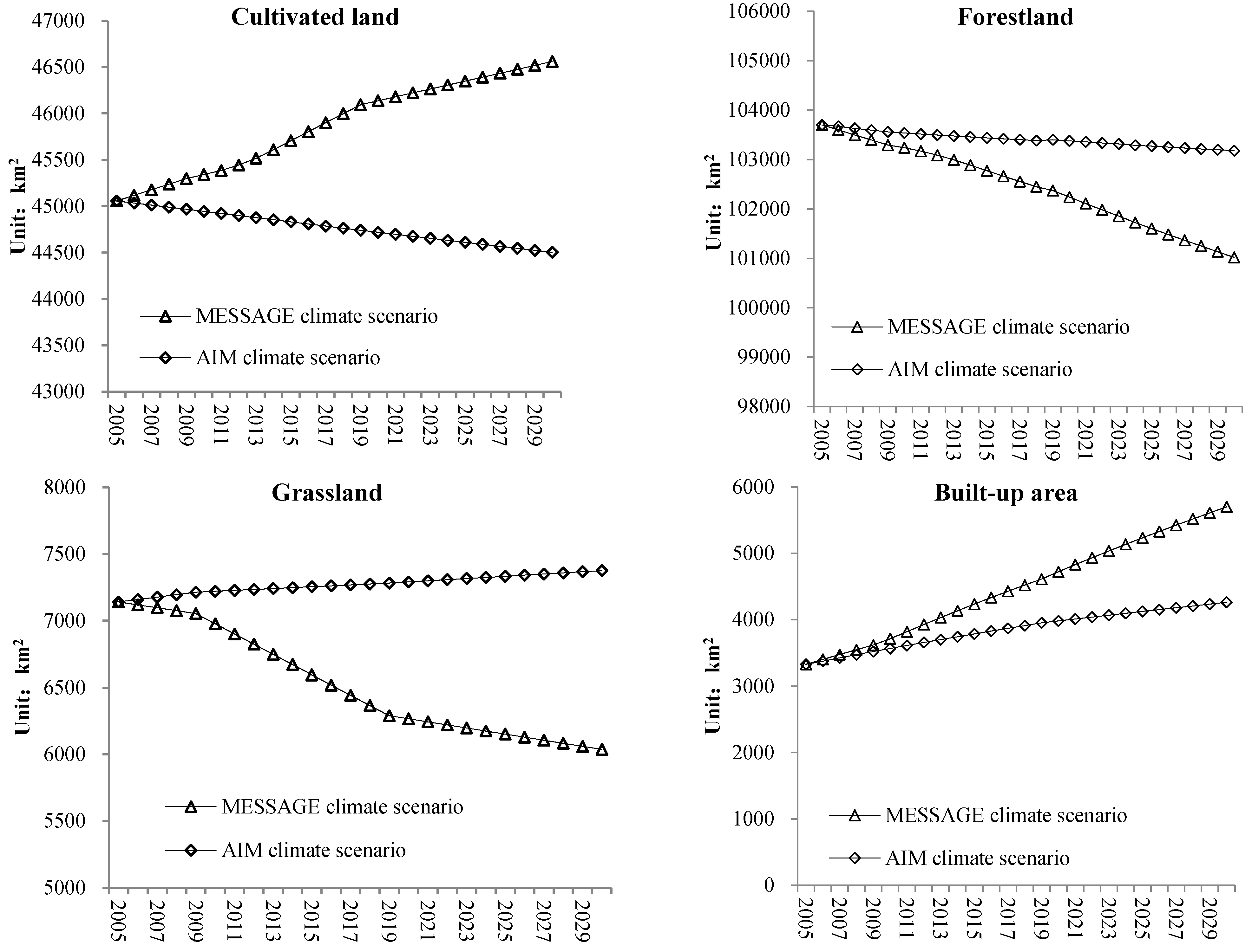
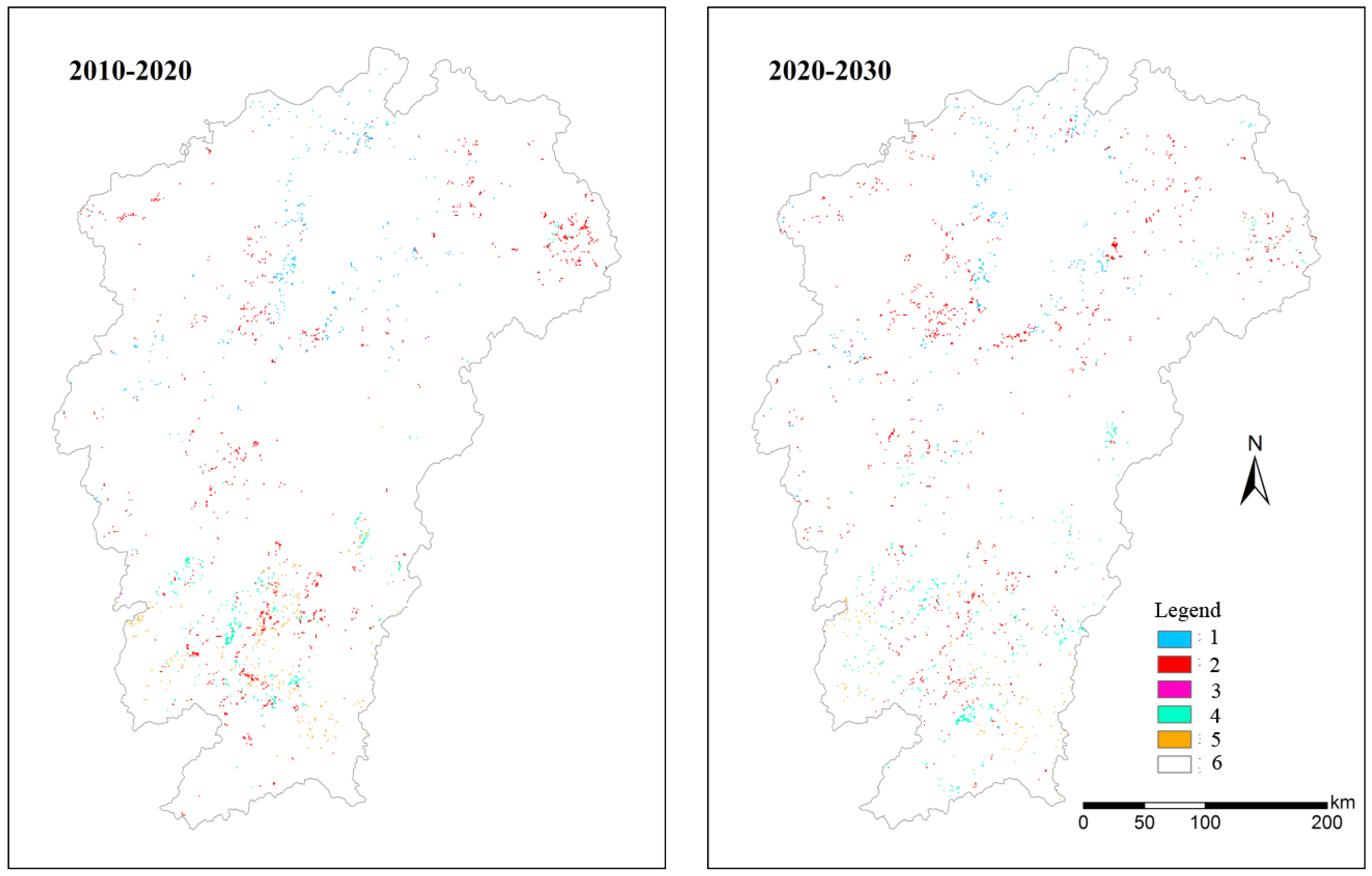
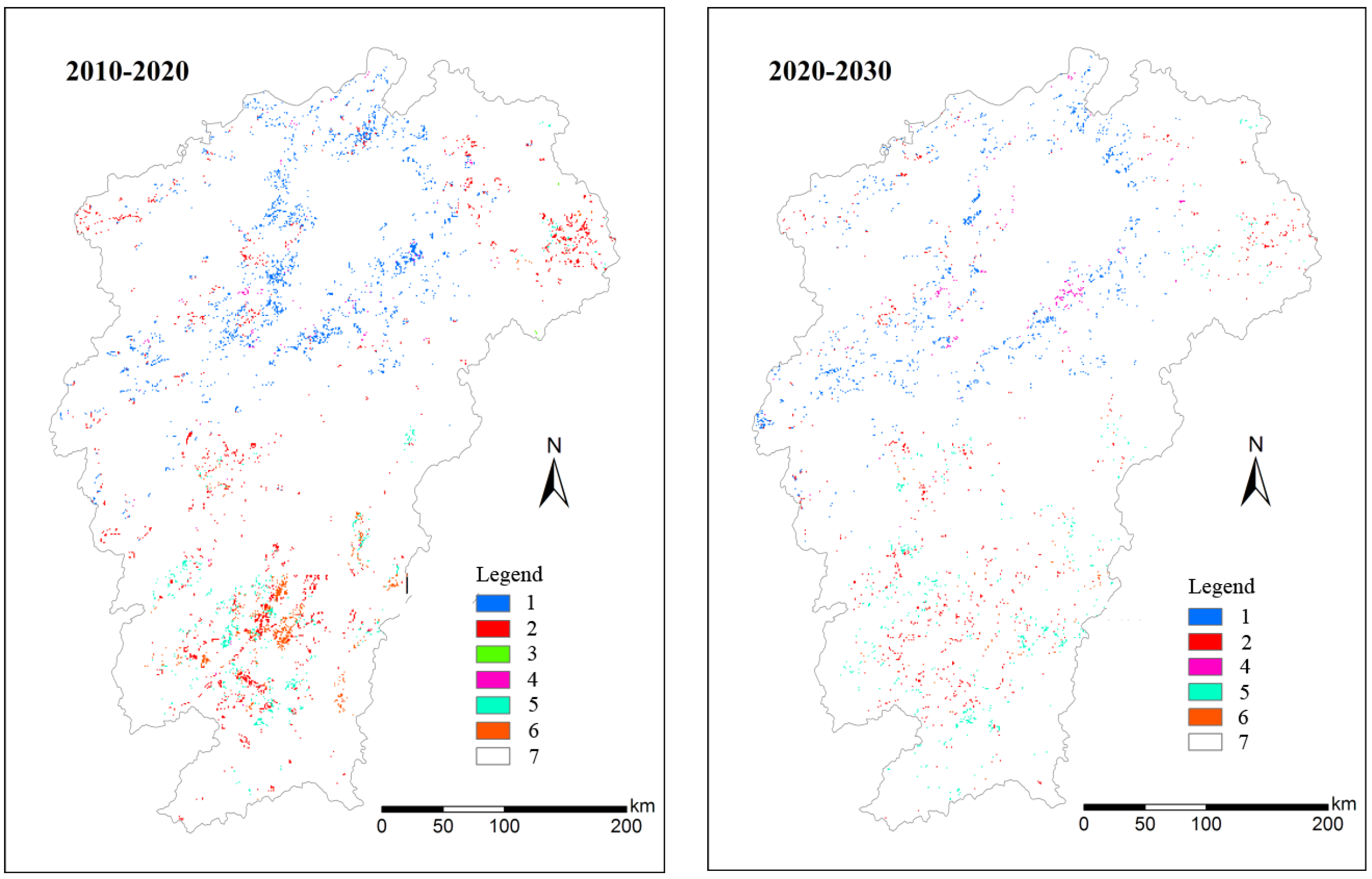
5.2. Analysis of the Simulation Results under the Asia-Pacific Integrated Model (AIM) Climate Scenario


5.3. Analysis of Simulation Results under the Model for Energy Supply Strategy Alternatives and Their General Environmental Impact (MESSAGE) Climate Scenario


6. Conclusions and Discussion
Acknowledgments
Author Contributions
Conflicts of Interest
References
- Foley, J.A.; DeFries, R.; Asner, G.P.; Barford, C.; Bonan, G.; Carpenter, S.R.; Chapin, F.S.; Coe, M.T.; Daily, G.C.; Gibbs, H.K.; et al. Global consequences of land use. Science 2005, 309, 570–574. [Google Scholar] [CrossRef] [PubMed]
- Arabatzis, G.; Christopoulou, O.; Soutsas, K. The EEC Regulation 2080/92 about forest measures in agriculture: The case of poplar plantations in Greece. Int. J. Ecodyn. 2006, 1, 245–257. [Google Scholar] [CrossRef]
- Liu, C.; Mullan, K.; Liu, H.; Zhu, W.; Rong, Q. The estimation of long term impacts of China’s key priority forestry programs on rural household incomes. J. For. Econ. 2014, 20, 267–285. [Google Scholar] [CrossRef]
- Arabatzis, G.; Mattas, K. The individual and social characteristics of poplar investors−cultivators and the factors that affect the size of poplar plantations according to the EU Regulation 2080/92. Agric. Econ. Rev. 2008, 9, 86–95. [Google Scholar]
- Arabatzis, G.; Klonaris, S. An analysis of Greek wood and wood product imports: Evidence from the linear quadratic Almost Ideal Demand System (AIDS). For. Policy Econ. 2009, 11, 266–270. [Google Scholar] [CrossRef]
- Zafeiriou, E.; Arabatzis, G.; Koutroumanidis, T. The fuelwood market inGreece: An empirical approach. Renew. Sustain. Energy Rev. 2011, 15, 3008–3018. [Google Scholar] [CrossRef]
- Kolovos, K.; Kyriakopoulos, G.; Chalikias, M. Co-evaluation of basic woodfuel types used as alternative heating sources to existing energy network. J. Environ. Prot. Ecol. 2011, 12, 733–742. [Google Scholar]
- Chalikias, M.; Kyriakopoulos, G.; Kolovos, K.G. Environmental sustainability and financial feasibility evaluation of woodfuel biomass used for a potential replacement of conventional space heating sources. Part I: A Greek Case Study. Oper. Res. 2010, 10, 43–56. [Google Scholar]
- Rose, S.K. Integrated assessment modeling of climate change adaptation in forestry and pasture land use: A review. Energy Econ. 2014, 46, 548–554. [Google Scholar] [CrossRef]
- He, J. Governing forest restoration: Local case studies of sloping land conversion program in Southwest China. For. Policy Econ. 2014, 46, 30–38. [Google Scholar] [CrossRef]
- Kyriakopoulos, G.; Kolovos, K.G.; Chalikias, M.S. Environmental sustainability and financial feasibility evaluation of woodfuel biomass used for a potential replacement of conventional space heating sources. Part II: A Combined Greek and the nearby Balkan Countries Case Study. Oper. Res. 2010, 10, 57–69. [Google Scholar] [CrossRef]
- Chen, Y.; Li, X.; Tian, Y.; Tan, M. Structural change of agricultural land use intensity and its regional disparity in China. J. Geogr. Sci. 2009, 19, 545–556. [Google Scholar] [CrossRef]
- Van Vuuren, D.P.; Stehfest, E.; den Elzen, M.G.J.; Kram, T.; van Vliet, J.; Deetman, S.; Isaac, M.; Goldewijk, K.K.; Hof, A.; Beltran, A.M.; et al. RCP2.6: Exploring the Possibility to Keep Global Mean Temperature Increase Below 2 °C. Clim. Chang. 2011, 109, 95–116. [Google Scholar] [CrossRef]
- Overmars, K.P.; Verburg, P.H.; Veldkamp, A. Comparison of a Deductive and All Inductive Approach to Specify Land Suitability in a Spatially Explicit Land Use Model. Land Use Policy 2007, 24, 584–599. [Google Scholar] [CrossRef]
- Valbuena, D.; Verburg, P.H.; Bregt, A.K.; Ligtenberg, A. An agent-based approach to model land−use change at a regional scale. Landsc. Ecol. 2010, 25, 185–199. [Google Scholar] [CrossRef]
- Clarke, L.; Edmonds, J.; Jacoby, H.; Pitcher, H.; Reilly, J.; Richels, R. Scenarios of Greenhouse Gas Emissions and Atmospheric Concentrations; Technical Report for U.S. Climate Change Science Program: Washington, DC, USA, 2007; p. 154.
- Sands, R.D.; Leimbach, M. Modeling agriculture and land use in an integrated assessment framework. Clim. Chang. 2003, 56, 185–210. [Google Scholar] [CrossRef]
- Jesper, S. Forest Tenure Reform in Asia and Africa—Local Control for Improved Livelihoods, Forest Management, and Carbon Sequestration; Bluffstone, R.A., Robinson, E.J.Z., Eds.; Resources for the Future Press: Washington, DC, USA, 2014. [Google Scholar]
- Jagger, P.; Luckert, M.M.K.; Duchelle, A.E.; Lund, J.F.; Sunderlin, W.D. Tenure and Forest Income: Observations from a Global Study on Forests and Poverty. World Dev. 2014, 64, S43–S55. [Google Scholar] [CrossRef]
- Moss, R.H.; Edmonds, J.A.; Hibbard, K.A.; Manning, M.R.; Rose, S.K.; van Vuuren, D.P.; Carter, T.R.; Emori, S.; Kainuma, M.; Kram, T.; et al. The next generation of scenarios for climate change research and assessment. Nature 2010, 463, 747–756. [Google Scholar] [CrossRef] [PubMed]
- Taylor, K.E.; Stouffer, R.J.; Meehl, G.A. An overview of CMIP5 and the experiment design. Bull. Am. Meteorol. Soc. 2012, 93, 485–498. [Google Scholar] [CrossRef]
- Van Vuuren, D.P.; Edmonds, J.; Kainuma, M.; Riahi, K.; Thomson, A.; Hibbard, K.; Hurtt, G.C.; Kram, T.; Krey, V.; Lamarque, J.F.; et al. The representative concentration pathways: An overview. Clim. Chang. 2011, 109, 5–31. [Google Scholar] [CrossRef]
- Meinshausen, M.; Smith, S.J.; Calvin, K.; Daniel, J.S.; Kainuma, M.L.; Lamarque, J.F.; Matsumoto, K.; Montzka, S.A.; Raper, S.C.; Riahi, K.; et al. The RCP greenhouse gas concentrations and their extensions from 1765 to 2300. Clim. Chang. 2011, 109, 213–241. [Google Scholar] [CrossRef]
- Ojima, D.; Emilio, M.; William, M. GLP (2005) Science Plan and Implementation Strategy; Technical Report for International Geosphere-Biosphere Program (IGBP): Stockholm, Sweden, 2005; p. 64. [Google Scholar]
- Climate Change 2007: The Physical Science Basis; Technical Report for the Fourth Assessment of Intergovernmental Panel on Climate Change: Geneva, Switzerland, 2007.
- Yu, R.; Wang, X.S.; Yan, Z.; Yan, H.M.; Jiang, Q.O. Regional Climate Effects of Conversion from Grassland to Forestland in Southeastern China. Adv. Meteorol. 2013, 9. [Google Scholar] [CrossRef]
- Jiang, Q.O.; Deng, X.Z.; Ke, X.L.; Zhao, C.H.; Zhang, W. Prediction and simulation of urban area expansion in Pearl River Delta Region under the RCPs climate scenarios. Chin. J. Appl. Ecol. 2014, 25, 3627–3636. (In Chinese) [Google Scholar]
- Rindfuss, R.R.; Walsh, S.J.; Turner, B.L.; Fox, J.; Mishra, V. Developing a science of land change: Challenges and methodological issues. Proc. Natl. Acad. Sci. USA 2004, 101, 13976–13981. [Google Scholar] [CrossRef] [PubMed]
- Lambin, E.F.; Geist, H.J. Land-Use and Land-Cover Change. Local Processes and Global Impacts; Springer-Verlag: Heidelberg, Germany, 2006. [Google Scholar]
- Verburg, P.H.; Overmars, K.P. Combining top-down and bottom−up dynamics in land use modeling: exploring the future of abandoned farmlands in Europe with the Dyna-CLUE model. Landsc. Ecol. 2009, 24, 1167–1181. [Google Scholar] [CrossRef]
- Verburg, P.H.; Eickhout, B.; Meijl, H.V. A multi-scale, multi-model approach for analyzing the future dynamics of European land use. Ann. Reg. Sci. 2008, 42, 57–77. [Google Scholar] [CrossRef]
- Briffa, K.R. Annual climate variability in the Holocene: Interpreting the message of ancient trees. Quat. Sci. Rev. 2000, 19, 87–105. [Google Scholar] [CrossRef]
- Farley, K.A.; Jobbágy, E.G.; Jackson, R.B. Effects of afforestation on water yield: a global synthesis with implications for policy. Glob. Chang. Boil. 2005, 11, 1565–1576. [Google Scholar] [CrossRef]
- Houghton, R.A. Revised estimates of the annual net flux of carbon to the atmosphere from changes in land use and land management 1850–2000. Tellus B 2003, 55, 378–390. [Google Scholar] [CrossRef]
- Canadell, J.G.; le Quéré, C.; Raupach, M.R.; Field, C.B.; Buitenhuis, E.T.; Ciais, P.; Conway, T.J.; Gillett, N.P.; Houghton, R.A.; Marland, G. Contributions to accelerating atmospheric CO2 growth from economic activity, carbon intensity, and efficiency of natural sinks. Proc. Natl. Acad. Sci. USA 2007, 104, 18866–18870. [Google Scholar] [CrossRef] [PubMed]
- Donohue, R.J.; Roderick, M.L.; McVicar, T.R. On the importance of including vegetation dynamics in Budyko’s hydrological model. Hydrol. Earth Syst. Sci. Discuss. 2007, 11, 983–995. [Google Scholar] [CrossRef]
- Odihi, J. Deforestation in afforestation priority zone in Sudano-Sahelian Nigeria. Appl. Geogr. 2003, 23, 227–259. [Google Scholar] [CrossRef]
- Deng, X.Z.; Huang, J.K.; Rozelle, S.; Uchida, E. Cultivated land conversion and potential agricultural productivity in China. Land Use Policy 2006, 23, 372–384. [Google Scholar] [CrossRef]
- Yan, D.; Schneider, U.A.; Schmid, E.; Huang, H.Q.; Pan, L.H.; Dilly, O. Impact of future climate change on land use change in Poyang Lake. Resour. Sci. 2013, 35, 2255–2265. (In Chinese) [Google Scholar]
- Zhang, L. Impact of climate change on geographical distribution of major tree species and natural vegetation in China. Ph.D. Thesis, Chinese Academy of Forestry Science, Beijing, China, 2011. [Google Scholar]
- Jiang, D.; Hao, M.M.; Fu, J.Y.; Zhuang, D.F.; Huang, Y.H. Spatial-temporal variation of marginal land suitable for energy plants from 1990 to 2010 in China. Sci. Rep. 2014, 4. [Google Scholar] [CrossRef] [PubMed]
- Jiang, D.; Zhuang, D.F.; Fu, J.Y.; Huang, Y.H.; Wen, K. Bioenergy potential from crop residues in China: Availability and distribution. Renew. Sustain. Energy Rev. 2012, 16, 1377–1382. [Google Scholar] [CrossRef]
- Ravindranath, N.H.; Somashekhar, B.S.; Gadgil, M. Carbon flow in Indian forests. Clim. Chang. 1997, 35, 297–320. [Google Scholar] [CrossRef]
- Masera, O.R.; Ordóñez, M.J.; Dirzo, R. Carbon emissions from Mexican forests: current situation and long-term scenarios. Clim. Chang. 1997, 35, 265–295. [Google Scholar] [CrossRef]
- Derek, B.; Stevenson, J.; Nelson, V. Does intensification slow crop land expansion or encourage deforestation? Glob. Food Secur. 2014, 3, 92–98. [Google Scholar]
- Wehner, S.; Herrmann, S.; Berkhoff, K. CLUENaban—A land use change model combining social factors with physical landscape factors for a mountainous area in Southwest China. Ecol. Indic. 2014, 36, 757–765. [Google Scholar] [CrossRef]
- Brandt, J.S.; Butsic, V.; Schwab, B.; Kuemmerle, T.; Radeloff, V.C. The relative effectiveness of protected areas, a logging ban, and sacred areas for old-growth forest protection in southwest China. Biol. Conserv. 2015, 181, 1–8. [Google Scholar] [CrossRef]
© 2015 by the authors; licensee MDPI, Basel, Switzerland. This article is an open access article distributed under the terms and conditions of the Creative Commons Attribution license (http://creativecommons.org/licenses/by/4.0/).
Share and Cite
Jiang, Q.; Cheng, Y.; Jin, Q.; Deng, X.; Qi, Y. Simulation of Forestland Dynamics in a Typical Deforestation and Afforestation Area under Climate Scenarios. Energies 2015, 8, 10558-10583. https://doi.org/10.3390/en81010558
Jiang Q, Cheng Y, Jin Q, Deng X, Qi Y. Simulation of Forestland Dynamics in a Typical Deforestation and Afforestation Area under Climate Scenarios. Energies. 2015; 8(10):10558-10583. https://doi.org/10.3390/en81010558
Chicago/Turabian StyleJiang, Qun'ou, Yuwei Cheng, Qiutong Jin, Xiangzheng Deng, and Yuanjing Qi. 2015. "Simulation of Forestland Dynamics in a Typical Deforestation and Afforestation Area under Climate Scenarios" Energies 8, no. 10: 10558-10583. https://doi.org/10.3390/en81010558