
Scheduling of Multiple Chillers in Trigeneration Plants

1
Department of Mechanical and Construction Engineering, Northumbria University, Newcastle upon Tyne NE1 8ST, UK
2
Atal Engineering Ltd, North Point, Hong Kong SAR, China
*
Author to whom correspondence should be addressed.
Energies 2015, 8(10), 11095-11119; https://doi.org/10.3390/en81011095
Submission received: 6 August 2015
/
Revised: 24 September 2015
/
Accepted: 28 September 2015
/
Published: 7 October 2015
(This article belongs to the Special Issue Tri-Generation Cycles, Combined Heat, Power and Cooling (CHPC))
Abstract
:The scheduling of both absorption cycle and vapour compression cycle chillers in trigeneration plants is investigated in this work. Many trigeneration plants use absorption cycle chillers only but there are potential performance advantages to be gained by using a combination of absorption and compression chillers especially in situations where the building electrical demand to be met by the combined heat and power (CHP) plant is variable. Simulation models of both types of chillers are developed together with a simple model of a variable-capacity CHP engine developed by curve-fitting to supplier’s data. The models are linked to form an optimisation problem in which the contribution of both chiller types is determined at a maximum value of operating cost (or carbon emission) saving. Results show that an optimum operating condition arises at moderately high air conditioning demands and moderately low power demand when the air conditioning demand is shared between both chillers, all recovered heat is utilised, and the contribution arising from the compression chiller results in an increase in CHP power generation and, hence, engine efficiency.
1. Introduction
Trigeneration systems have received substantial attention recently mainly because they have the potential to utilise summer waste heat from combined heat and power plant that would otherwise be wasted. Most recently, attention has mainly focused on the development of small systems for residential and small commercial applications (e.g., [1,2,3]). For a more detailed review of recent developments, see Chua et al. [4]. This work concerns itself with the part-load behaviour of trigeneration plants of capacities applicable to commercial applications with particular regard to load sharing between absorption cycle and compression cycle chillers.
Most small- and medium-scale trigeneration plants with electrical capacities of under 5 MWe consist of one or more combined heat and power (CHP) modules with heat recovery to a pressurised hot water circuit which services a combination of building heating demands and a heat-driven absorption cycle chiller plant for air conditioning. Thus, with electrical power, trigeneration is accomplished. At these electrical capacities (i.e., up to around 5 MWe) the CHP prime mover of choice is currently a natural gas (or syngas) fired reciprocating internal combustion engine because they tend to offer superior power generating efficiencies in most applications unless ambient air temperatures are extremely (and consistently) low (in which case gas turbines may compete). The singular disadvantage of using reciprocating engines in trigeneration plants with absorption cycle chillers is that part of the engine heat recovery (i.e., jacket wall and oil cooler) is realised at relatively low temperatures with maximum jacket cooling inlet temperatures of typically 97 °C (or lower particularly in smaller CHP modules) [5]. At these temperature limits, application is restricted to the lower-performing single-effect absorption cycle chiller.
These engines are controllable such that power generating capacity can be varied in response to variations in electrical demand. There is a cut-off below which the engine is not permitted to operate due, in part, to a rapid decline in efficiency. This cut-off is conventionally 50% of the rated electrical generating capacity. As the CHP module turns down to meet a declining electrical demand, there is a decline in efficiency the rate of which increases as the demand falls. Some of this decline in electrical generating efficiency can be recovered as waste heat which results in the heat recovery “efficiency” increasing as the electrical generating efficiency falls.
In circumstances during which the electrical demand falls at a time when the demand for air conditioning is high and cannot be met using the available waste heat from the CHP modules, there is an argument for having a contribution to air conditioning coming from electrical vapour-compression chillers (instead of using boilers to provide additional top-up heat for use by the absorption cycle chillers). In this way, the CHP module’s electrical generating capacity increases to meet the air conditioning load and, in doing so, operates at a higher electrical generating efficiency than would otherwise be the case. There is, therefore, a case to be made for using both absorption and compression chillers in trigeneration plants. Conventionally, compression chillers are usually only used (if at all) in these plants to meet minor air conditioning demands in mid-season that would otherwise be below the turn-down capacity of the absorption cycle chiller. In this paper, we argue that both types of chiller should be routinely used and both should be sized to achieve optimum overall plant performance.
The aim of the research is to develop a procedure for scheduling the air conditioning load between absorption and compression chillers in trigeneration plants. This will be achieved through the following objectives:
- Modelling of a conventional single-effect absorption cycle chiller and centrifugal compression chiller with sufficient detail to capture part-load performance characteristics.
- Simplified modelling of gas-fired reciprocating internal combustion engine-based CHP modules.
- Verification of the various models with typical manufacturers’ performance data.
- Develop an algorithm for optimally scheduling the air conditioning demand between absorption and compression chillers.
- Apply the algorithm to a practical plant configuration case study and evaluate the results.
Of the two CHP module control strategies, a heat-led strategy is one where the CHP module is controlled based on the heating demand and any surplus power generated is exported to the grid connection. A power-led strategy is one where the CHP module is controlled based on the host building power demand and unutilised heat recovery is rejected. The control strategy adopted is largely dependent on economics which, in turn, will depend on local fuel prices, any government incentives and tax exemptions, etc. [6,7]. For instance, a trigeneration economic analysis by Mago and Chamra [8] concluded in favour of a heat-led and a hybrid heat/power-led strategy on economic grounds. Their analysis used typical USA energy prices ruling in 2009 with a ratio of electricity to fuel price of 2.8. The same ratio in the UK in 2009 was typically >4.1 [9] meaning that electricity is more economically dominant in UK conditions. Therefore, a power-led strategy will usually be the most economic approach for commercial buildings in the UK with heat-led only generally used in domestic micro-CHP applications [10]. The work reported here will therefore be confined to power-led trigeneration plants in which no intentional export of electrical power takes place (but electrical import from the grid is available).
2. Review
Cardona and Piacentino [11] were among the first to investigate the load sizing of absorption cycle and compression cycle chillers in trigeneration plant but they did this without considering the detailed part-load performance of the chillers. Most of the recent research on trigeneration economics has mainly focused on the energy or cost management of the CHP plant predominantly when used with absorption cycle chillers but also when using either absorption cycle chillers or compression chillers. Lozano et al. [12] related the operating strategy of the cooling production plant to the operating cost and fuel prices, and identified a profitable fuel price range for either the absorption cycle chiller or electrically-driven compression chiller to provide air conditioning. However, the influence of the size of the primary and auxiliary cooling plant is not investigated. Piacentino et al. [6] investigate the design of trigeneration plants serving clusters of buildings through the development of an optimisation algorithm targeting the net present value of the plant and applied the new algorithm to a cluster of four buildings taking into account local energy prices and tax exemptions [7]. In later work they carried out a sensitivity analysis to investigate the effects of tax exemption for the fuel consumed by CHP in trigeneration plants, observing an increase in tax exemption encouraged a larger optimal size of the cogeneration unit and the absorption cycle chiller but also increased the amount of heat annually wasted as consequence [13]. Chicco and Mancarella [14] developed a new performance indicator—“trigeneration primary energy saving” (TPES)—to evaluate the primary energy savings from different plant combinations comprising absorption cycle chillers, reciprocating vapour-compression chillers and a directly-fired absorption cycle chiller option. They found that using the electrically-driven chiller and directly-fired chiller provided more economic cooling than using a waste heat absorption cycle chiller when the heating demand is high and the coefficient of performance (CoP) of the electrically-driven and directly-fired chillers are high.
Regarding control strategies, Mago and Chamra [8] evaluated trigeneration plants undergoing both heat-led and power-led control as well as a hybrid method in a basic system consisting of a CHP module, absorption cycle chiller and auxiliary boiler. They quantified the benefits of using the hybrid strategy over the other two conventional strategies in terms of the primary energy consumption, operating cost and emission. Kavvadias et al. [15] summarised three other commonly used operating strategies including continuous operation, peak-shaving and base load operation. Facci et al. [16] used dynamic programming to investigate optimum control of trigeneration plants over short time horizons (one day). Transfer function models of the various plant components appear to have been used but few details are supplied and, of course, transfer functions models are usually limited to a finite range of operational behaviour due to plant nonlinearities.
As far as the cooling demand is concerned, Kavvadias et al. [15] suggested that any additional electricity consumed by auxiliary cooling plant should be considered using optimisation (which is the subject of the present work) and suggested that an electrical equivalent load strategy should be used instead of the basic power-led control strategy to offer better peak electricity demand smoothing of the trigeneration system. In related work, Kavvadias and Maroulis [17] used multi-objective function optimisation to find maxima for the net present value, primary energy saving ratio and emissions reduction ratio in trigeneration plants with both absorption cycle and compression cycle chillers. They applied their method to a case study applicable to the Greek energy market with fluctuating fuel and electricity prices however the part-load performance characteristics of the chillers was not accounted for.
For economic assessments, the impact of fuel prices, energy tariffs and tax exemptions on the operation strategy is acknowledged. The importance of using the electricity to gas cost ratio (EGCR) to determine an appropriate operating strategy regarding the allocation of the cogenerated heat (to satisfy the cooling or heating demands) has been addressed by Kong et al. [18,19]. They concluded that the optimal operating strategy is independent of the fuel price when the EGCR is high (other work in this area was also reported by Lozano et al. [12] but only for a fixed thermal load).
It is clear that little attention has been given to the optimised sharing of cooling load between absorption cycle and compression cycle chillers in trigeneration plants taking into account the part-load performance characteristics of the plant—what we refer to in the present work as load scheduling. A study of this aspect therefore forms the basis of the work reported here. The main emphasis of the work reported here and its departure from the work previously reported and summarised above lies in the rigorous modelling of the refrigeration plant in order to capture the underlying performance characteristics when operating at part-load.
3. Modelling
A modelling method of intermediate complexity is used—simple steady-state descriptions of each piece of plant (absorption cycle chiller, compression cycle chiller and CHP module) but with sufficient detail to enable part-load performance behaviour of each to be captured. The complete system to be described is illustrated in Figure 1.
Figure 1.
Trigeneration system.

At the multi-MW scale of the plant capacities involved in this work, it is not feasible to contemplate laboratory-scale validation and only field trial testing may be possible. However, the latter approach would merely lead to typical operational behaviour over prevailing load conditions and would likely involve significant measurement uncertainty (it would not be possible to operate the plant in field conditions to a prescribed experimental plan with controlled boundary conditions). As a compromise therefore, attempts are made in the following to cross check the results of the two chiller models reported here using typical results from manufacturers of large scale chillers.
3.1. Vapour-Compression Chiller
A steady-state model is developed with the following assumptions and limitations:
- Evaporator and condenser refrigerant outlet states are assumed to be saturated (i.e., superheating and sub-cooling effects are not considered).
- Refrigerant pressure losses are neglected.
- In this work, the refrigerants used are taken to be azeotropic compounds.
At the capacity scale typically encountered in commercial trigeneration plants where the vapour compression chiller contribution to load may be high, centrifugal compression technology is most likely to be encountered. The chiller model developed here therefore is based on a high speed (up to 40,000 RPM) centrifugal chiller of the type currently being developed for oil-free (magnetic bearing) compressors [20]. The modelling method adopted broadly follows the approach developed by Bourdouxhe et al. [21].
The cooling load, Qe, is specified.
For the condenser, the saturated condensing temperature is obtained from the following:
from which the condensing pressure is obtained from refrigerant properties:
Likewise for the evaporator:
But it is more convenient to express the evaporating temperature, Te,sat, in terms of the (specified and constant) chilled water outlet temperature from the evaporator:
from which the evaporating pressure is obtained from refrigerant properties:
The required refrigerant mass flow rate is then obtained by an energy balance on the evaporator:
in which, from refrigerant properties:
Based on a backward-curve impeller rotating at N (RPS) with a peripheral velocity of U (m·s−1) it is possible to show that the volume flow rate of refrigerant at the impeller inlet, Vimp,i, can be obtained from the following [21]:
in which
The overall pressure ratio, rP, includes the impeller and its discharge diffuser (i.e., the complete compressor assembly). The pressure ratio for the impeller section only, rP,imp, is obtained from the following [21]:
in which, from refrigerant properties:
The refrigerant mass flow rate is obtained from the following (note that the refrigerant mass flow rate is also obtained in Equation (5) from an evaporator heat balance):
in which,
Thus the work imparted to the impeller is obtained from the following:
And the overall compressor power consumption can be obtained from [21]:
In Equation (10), it is assumed that the various compressor losses can be described by a fixed loss component, Wloss,fixed, comprising mainly electrical motor losses (resistive motor winding losses, etc.) and variable electromechanical losses which are assumed to be in proportion to the impeller power according to the loss factor, α.
The compressor inlet temperature is obtained from the following in which the refrigerant mass flow rate is obtained from Equation (8):
in which, from refrigerant properties:
The compressor efficiency and plant coefficient of performance are now obtained from Equations (12) and (13).
Finally the outlet condenser cooling water temperature and inlet chilled water temperature are obtained:
Note Wloss,fixed does not appear in Equation (14) because this component is considered as a loss to the ambient environment and is not transferred to the refrigerant.
Equations (1)–(11) were coded into two Matlab functions (a parent function containing Equations (1)–(5) and a compressor function containing Equations (6)–(11)). The solution procedure is summarized in the algorithm given below.
| Algorithm |
|
Refrigerant properties were calculated using NIST REFPROP v7 [22] by means of NIST’s Matlab function, ‘refpropm’.
3.1.1 Verification
To check the results predicted by the model, manufacturer’s data are compared in Figure 2 with results predicted by the model described above. It must be stressed here that this is not an attempt at model validation because some of the model parameter assumptions could not be cross-matched with the manufacturer’s data (some were unavailable and others were commercially protected). This comparison is done merely to show that the performance characteristics predicted by the model are broadly similar to what might be expected from a commercially available plant. The plant is an 892.25 kW (design capacity) oil-free centrifugal compressor driven chiller as described by Yik et al. [20]. The chilled water outlet temperature set point is 7 °C and the results show performances at alternative condenser cooling water inlet temperatures of 22 °C, 27 °C and 32 °C. The mass flow rates of chilled water and condenser cooling water are 38.06 kg·s−1 and 50 kg·s−1 respectively. The refrigerant is R134a. Other parameter assumptions used in the model but which could not be cross-matched to the manufacturer’s details are as follows:
εe = εc = 0.75, D = 0.1m, w = 0.014m, β = 130°, Wloss,fixed = 5kW, α = 0.24
Figure 2.
Vapour compression chiller behaviour. (a) Tclgw,i = 32 °C; (b) Tclgw,i = 27 °C; (c) Tclgw,i = 22 °C.
Figure 2.
Vapour compression chiller behaviour. (a) Tclgw,i = 32 °C; (b) Tclgw,i = 27 °C; (c) Tclgw,i = 22 °C.

The results confirm an expected pattern of part-load behaviour of vapour compression chillers in that the performance does not peak at rated conditions but at some intermediate point along the part-load spectrum.
3.2. Absorption Cycle Chiller
As in the previous case, a steady-state model is developed with the following assumptions and limitations:
- Evaporator and condenser refrigerant outlet states are assumed to be saturated (i.e., superheating and sub-cooling effects are not considered).
- Refrigerant pressure losses are neglected.
As has been noted [5], a single-effect absorption cycle refrigeration plant is used due to the limited heating water temperatures available from reciprocating internal combustion engine CHP prime movers. Best performances in plants of this type will accrue from the water and aqueous lithium-bromide refrigerant/absorbent combination which is the adopted fluid pair used here.
The modelling method adopted broadly follows the approach developed by Bourdouxhe et al. [21]. The main difference here is that cooling load, Qe, is specified with an initial estimate of the absorber, Qa, and condenser, Qc, loads which means that the generator load is obtained by an overall cycle heat balance. The algorithm will therefore seek a converged solution through Qa and Qc.
The absorber and condenser are cooled in series in this model. Thus, the condensing temperature is obtained from the following in which Tclgw,i is the cooling water temperature entering the absorber:
Again the constant chilled water outlet temperature from the plant will be specified so the evaporating temperature, evaporating pressure and refrigerant mass flow rate are obtained as in the previous case (Equations (3)–(5)).
The temperature of the absorber solution is obtained from the following (which therefore forms the solution temperature at the absorber outlet):
The generator load is obtained from an overall heat balance (Equation (18)) and, hence, the generator solution is obtained from Equation (19) which forms the generator solution outlet temperature.
The solvent-strong solution concentration is obtained from the equilibrium properties of lithium-bromide solution [23]:
At design-rated capacity, the design solvent-weak solution concentration is obtained similarly (Equation (21)) and the corresponding mass flow rate of strong solution is found from a lithium bromide mass balance about either the absorber or generator (which reduces to Equation (22)), from which the design weak solution mass flow is then obtained (Equation (23)):
in which is the design weak solution mass flow rate, kg·s−1.
At part load, if the (pumped) weak solution flow rate is varied as some proportion, p, of the design value, the weak solution concentration and solution mass flow rates are alternatively obtained from the following:
Solution enthalpies were determined using fluid properties [24]. For the generator and absorber outlet solution (Equations (27) and (28)):
In accordance with conventional practice, a solution heat exchanger (recuperator) is used to precool the strong solution prior to entering the absorber whilst correspondingly preheating the weak solution prior to entering the generator. The temperature of the strong solution entering the absorber is obtained from the heat exchanger effectiveness, εhx, and, hence, the corresponding entering solution enthalpy is obtained from fluid properties [24]:
The temperature of the refrigerant vapour leaving the generator is assumed to be the same as the equilibrium solution temperature at the solution/vapour interface. In turn, this is assumed to be at the lower (entering) weak solution concentration. From this temperature together with the condensing pressure, the enthalpy of this refrigerant vapour is obtained:
Finally, a curve-fit to the solidus line found in the equilibrium data for solutions of lithium bromide [23], provides limiting values of strong concentration and temperature at which solid crystals of lithium bromide might be expected to present. The most vulnerable site for this will be at the outlet strong solution connection of the solution heat exchanger where the solution is at its highest concentration and lowest temperature. (Note that, in this work, the ‘strong’ solution implies strong in solvent not refrigerant.) This calculation is done during simulations to flag up a warning of impending crystallisation and it is expressed by the variable ΔXcrit—the difference between the solidus concentration (in percent) and the actual concentration (i.e., a negative result implies crystal formation and a positive result implies a liquid state). The calculation is carried out using Equation (33).
Algorithm
Equations (3), (4) and (16)–(32), together with the equations described below were coded into a further Matlab function and the following iterative solution procedure was included. The solution procedure is broadly in accordance with that developed by Bourdouxhe et al. [21].
Step 1. Input the target cooling load (Qe) and first approximations for the condenser and absorber loads (Qc, Qa). Input the target chilled water outlet temperature and the boundary conditions (inlet cooling water and generator heating water temperatures and chilled water, cooling water and generator heating water mass flow rates). Input the heat exchanger effectivenesses (εe, εc, εa, εg, εhx). Solve Equations (16)–(32).
Step 2. Calculate zero functions based on energy balances about the absorber and generator:
Step 3. Form the 2 × 2 Jacobian matrix as follows:
The zero functions (Equations (34) and (35)) are thus differentiated with respect to the current absorber and condenser heat loads using a simple numerical discretisation scheme (Equations (36)–(39)) based on a user-supplied heat transfer interval value, ΔQ. In practice, the latter will be selected by trial-and-error as a compromise between accuracy and computational effort. In the present work, a value of 5 kW was found to be satisfactory for the typically multi-MW loads applied in Section 5 and led to convergence errors of less 0.1%.
Thus the Jacobian matrix is re-formed at each iterative sweep to form Equation (40).
Step 4. Update Qa, Qc as follows:
in which:
The inverse of the Jacobian matrix is obtained and the result is used to multiply the current zero function vector (a 2 × 1 vector in this case). The result is then deducted from the current estimates of the absorber and condenser heat loads to produce new estimates of these values (Equation (41)). Essentially, this is a multivariable Newton-Raphson algorithm.
Step 5. Repeat the procedure from Step 2 until two successive values of Qa, Qc agree to within an acceptable tolerance.
Step 6. Conclude the simulation by calculating the cycle coefficient of performance and all outlet water temperatures:
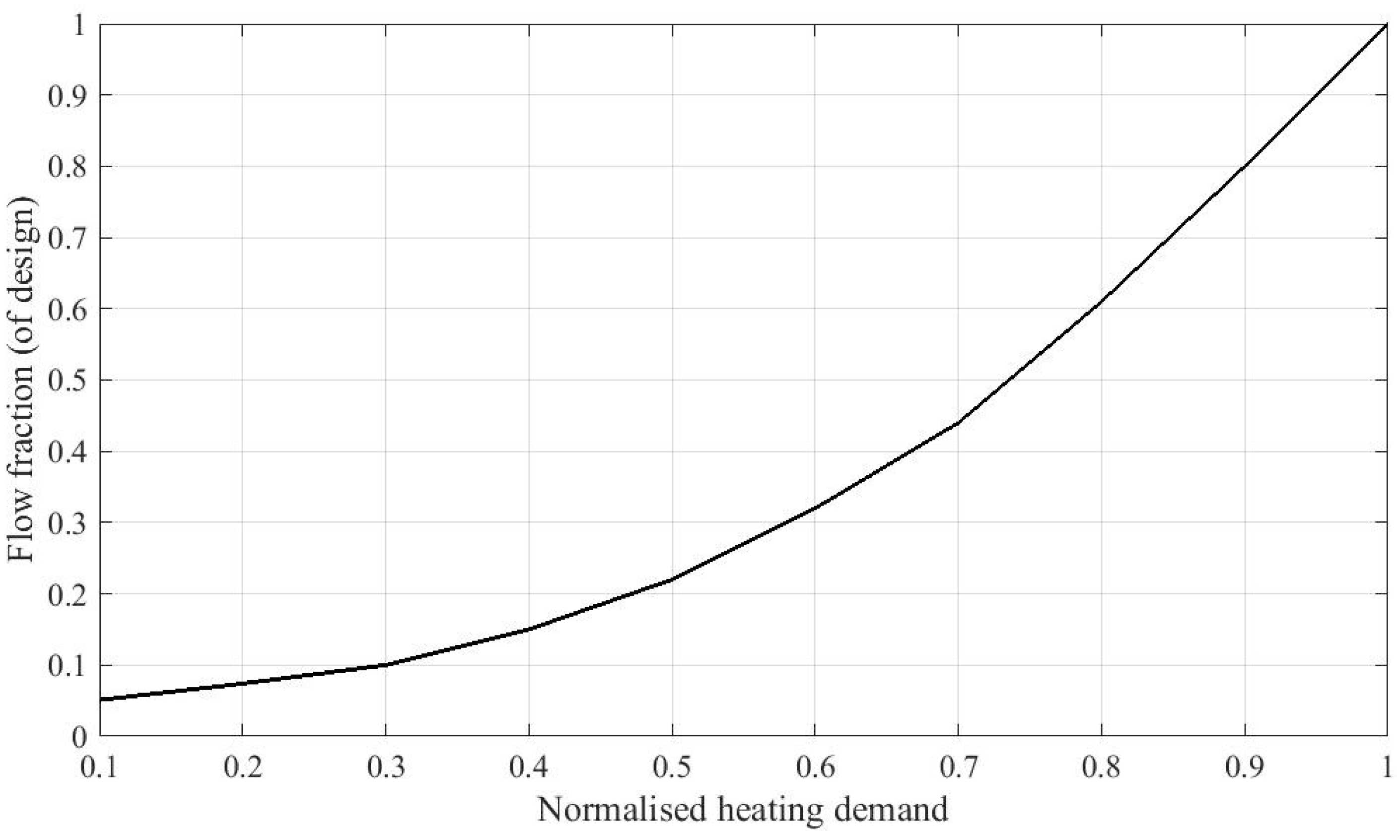
As far as control is concerned, normal practice is to vary the generator heat input in response to variations in cooling demand. In plants with generators heated using hot water, the conventional approach would be to vary the flow rate of hot water to the generator in response to variations in evaporator chilled water outlet temperature. The control valve used to perform this will usually have an equal percentage characteristic [25] for hot water (linear, when steam is used). Therefore, a part-load simulation of the absorption cycle chiller will start with a simulation at design-rated conditions (mghw at the design value and m’sw determined using Equation (23)) and for part load simulations mghw is varied from its design value in proportion to the installed characteristic of an equal percentage control valve as shown in Figure 3 constructed at typical practical values including a valve authority of 0.5. Some manufacturers of these plants also vary the pumping rate of the weak solution as some function of the load proportion. This can be adjusted through the variable p in Equation (24) however in the present work it was assumed that this flow rate remained constant at its design value for all part load conditions.
Figure 3.
Generator heating valve characteristic.

3.2.1 Verification
Two verification tests were carried out based on preliminary results from the absorption cycle chiller model described above. The first involved a comparison with results from a single example case study presented by American Society of Heating, Refrigerating and Air Conditioning Engineers (ASHRAE) [26]. The second involved a comparison with part-load performance data for a single-effect water and lithium bromide solution chiller published by a manufacturer. The first test involved a direct comparison with identical boundary conditions and parameters whereas the second is merely an outline verification to show whether the part-load behaviour predicted by the model is broadly similar to the characteristics evident in commercially-available plant. Input data for the first comparison test are given in Table 1 [26] and the results are compared in Table 2.

Table 1.
Comparison test case—input data [26].
| Variable | Value |
|---|---|
| Qe | 2148 kW |
| Tchw,i/Tchw,o | 12/6 °C |
| Tclgw,i/Tclgw,a,o/Tclgw,o | 27/31.5/35 °C |
| Thw,i/Thw,o | 125/115 °C |
| msw | 12 kg·s−1 |
| mew | 85.3 kg·s−1 |
| mcw | 158.7 kg·s−1 |
| mghw | 74.4 kg·s−1 |
| εhx | 0.654 |
| εe * | 0.588 |
| εc * | 0.238 |
| εa * | 0.328 |
| εg * | 0.465 |
* ASHRAE effectiveness deduced from other input data.
| Variable | ASHRAE result [26] | Result from present work | Difference and% difference (Base = [26]) |
|---|---|---|---|
| Qa | 2984 kW | 2973 kW | −11 kW (−0.37%) |
| Qc | 2322 kW | 2298 kW | −24 kW (−1.03%) |
| Qg | 3158 kW | 3123 kW | −35 kW (−1.11%) |
| CoP | 0.68 | 0.69 | 0.01 (1.47%) |
| Xs | 64.6% | 64.7% | 0.1% (0.16%) |
| Xw | 59.6% | 59.7% | 0.1% (0.16%) |
| Te,sat | 1.8 °C | 1.8 °C | 0 (0%) |
| Tc,sat | 46.2 °C | 46.0 °C | −0.2 K (−0.43%) |
| Tsg,o | 103.5 °C | 103.8 °C | 0.3 K (0.29%) |
| Tsa,o | 40.7 °C | 40.7 °C | 0 (0%) |
| ΔXcrit | (Not given) | 1.3% | - |
The second test case compares the results of the model under part-load conditions with part-load performance data published by a manufacturer for a long-established single-effect water and aqueous lithium bromide plant [27]. The commercial plant has a design rated cooling capacity of 1011 kW at a chilled water outlet temperature of 6.67 °C. The chilled water mass flow rate is 43.5 kg·s−1 and the cooling water mass flow rate 66.7 kg·s−1. The generator heating water flow rate is 75 kg·s−1 (variable with capacity). However most of the other parameters were unavailable and so the values used in the ASHRAE test case were re-used here. These results, therefore, are merely indicative of the part-load characteristic to be expected from this type of plant and do not imply model validity. The results are given in Figure 4. The commercial data are plotted for two alternative cooling water inlet temperatures (23.8 °C and 29.4 °C) whereas the results generated by the model are based the average of these two values (26.6 °C).
The results of the first test case show that the model gives a good agreement with results carried out using an alternative calculation method [26]—Table 1. The results of the part-load performance test case show that the model has part load behaviour which is consistent with commercially-available plant of a type similar to that described by the model (Figure 4). The average of the percentage root-mean-square error values of the reference data and the model-predicted results is 3.24%. Like the vapour-compression chiller, it is evident that peak performance of these plants occurs not at rated conditions but at some intermediate value on the part-load spectrum (here, typically around 50% of design-rated capacity).
Figure 4.
Absorption cycle chiller behaviour ([27], and present work).
Figure 4.
Absorption cycle chiller behaviour ([27], and present work).

3.3. Combined Heat and Power Plant
In most small-to-medium applications of trigeneration, reciprocating internal combustion gas engines tend to be the prime mover of choice mainly due to superior power generating efficiency when compared with other options. At higher capacities (above about 300 kWe) these engines are turbo-charged lean-burn and operate at moderate speed (3000 RPM) consistent with conventional two-pole generators. These engines when used in CHP plant are usually able to module in the capacity range 0.5,1. Manufacturers’ usually supply performance data which gives the power output and recoverable heat output at part-load ratios, PLR, of 1 (rated), 0.75, and 0.5. In this work, we take the part-load performance data at these three points for an example set of CHP module engines and fit quadratic “best fit” curves to the efficiency and heat recovery utilisation (sometimes referred to as “heat efficiency”) data as a function of the part load ratio, PLR.
The fitted equations take the form of Equations (46) and (47).
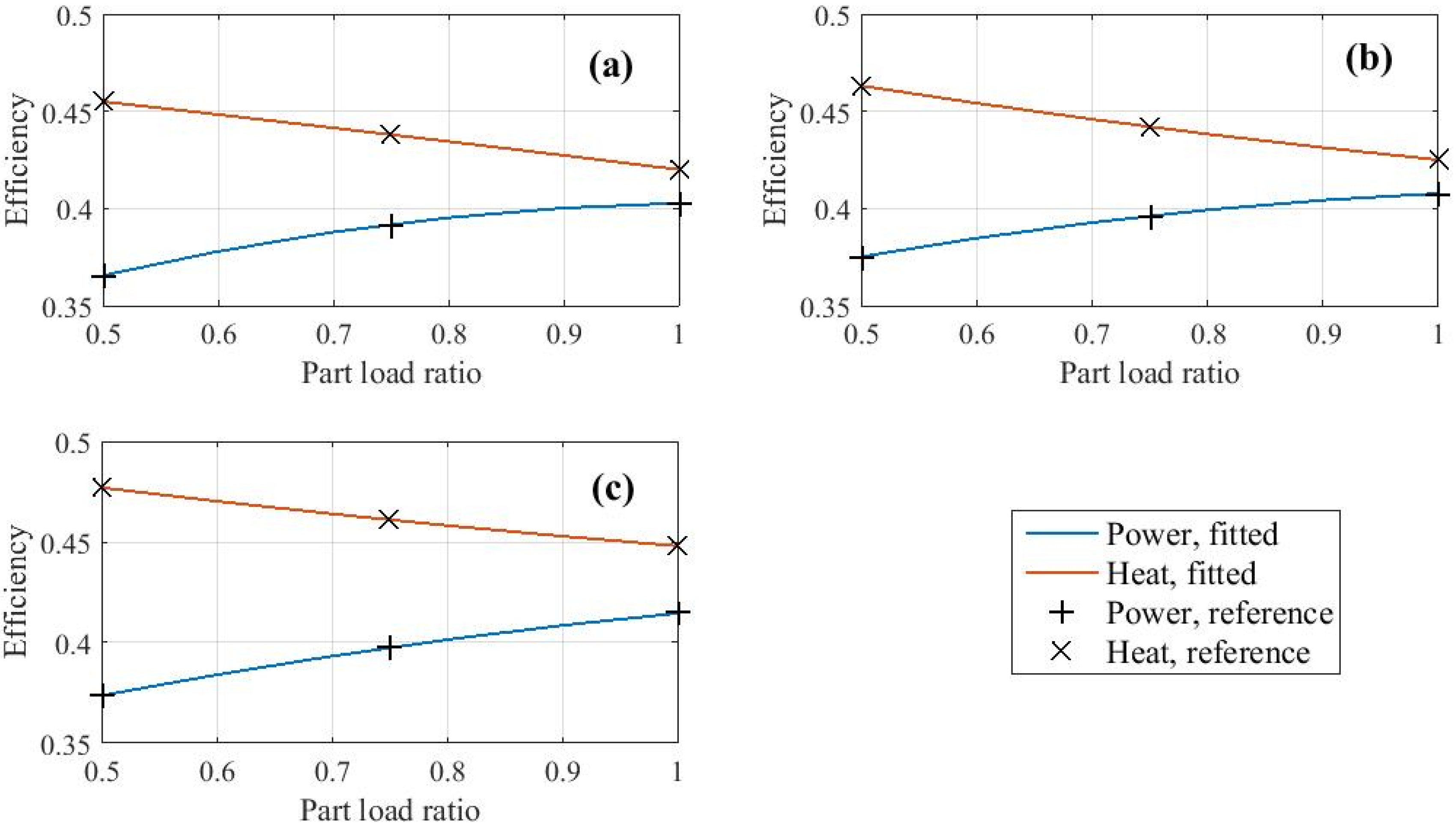
Results of fitting to an example set of three commercially-available CHP module gas engines [28] are given in Table 3 and Figure 5, in which ηp and ηh are the electrical power efficiency and heat recovery utilisation respectively. (Figure 5 confirms that the heat recovery utilisation increases as the electrical power efficiency reduces due to an increasing proportion of the losses being recovered as heat).
Table 3.
Efficiency and heat utilisation of example CHP modules [28]—model fitting.
| Rated kWe | PLR | ηp | ηh | Ap | Bp | Cp | Ah | Bh | Ch |
|---|---|---|---|---|---|---|---|---|---|
| 499 | 1 | 0.403 | 0.420 | 0.267 | 0.260 | −0.124 | 0.486 | −0.058 | −0.008 |
| 0.75 | 0.392 | 0.438 | |||||||
| 0.5 | 0.366 | 0.455 | |||||||
| 1063 | 1 | 0.408 | 0.425 | 0.305 | 0.179 | −0.076 | 0.518 | −0.126 | 0.033 |
| 0.75 | 0.396 | 0.442 | |||||||
| 0.5 | 0.375 | 0.463 | |||||||
| 1790 | 1 | 0.415 | 0.448 | 0.306 | 0.163 | −0.054 | 0.518 | −0.094 | 0.024 |
| 0.75 | 0.398 | 0.461 | |||||||
| 0.5 | 0.374 | 0.477 |
Figure 5.
Quadratic model fitting to example [17] CHP engines. (a) 499 kWe module; (b) 1063 kWe module; (c) 1790 kWe module.
Figure 5.
Quadratic model fitting to example [17] CHP engines. (a) 499 kWe module; (b) 1063 kWe module; (c) 1790 kWe module.

4. Scheduling Algorithm
The two CHP engine Equations (46) and (47) were coded into a Matlab function which forms the parent function for those described in Section 3.1 and Section 3.2. The parent functions receives a target power demand to be met by the CHP module (a value which lies within its generating range), a target cooling demand to be met, and all of the boundary conditions and model parameters described in the previous sections for the two chillers and the CHP module.
Two cost functions are defined as follows; one of these describing financial saving and the other describing carbon saving. The savings described are with reference to a conventional situation in which all electricity is imported from a grid connection, heating demands are met by fuel-fired boilers and air conditioning demand is met by a vapour compression chiller using grid-imported electricity.
For the financial saving cost function, the instantaneous cash saving due to the trigeneration plant operating at a defined set of boundary conditions and power, heating and cooling demands, is given by Equation (48) assuming that no electricity generated by the CHP module is exported:
To define an optimisation problem, we seek a cost function that requires to be minimised. Thus Equation (48) in inverted after dividing through by the electricity import price, Pe,im. The resulting cost function, CFmoney, is then arbitrarily scaled by 100 so that results are finite but non-negligible (Equation (49)):
where are fuel/electricity price ratios for boiler plant and CHP respectively.
Equations (48) and (49) can either be interpreted as the cost and cost factor over a specified period of plant operation (in which case electricity, fuel and heat loads are defined in kWh) or as an instantaneous cost and cost factor (in which case the loads are in kW). In the application presented in Section 5, the latter interpretation is used so that results across a range of load factors can be arrived at, thus capturing plant performance across a full turn-down cycle.
It is possible to define an alternative carbon emission cost function, CFcar, in exactly the same way as in the above where ff,bp and ff,chp are replaced with ff,car (the fuel/electricity carbon emission intensity ratio assuming that the boiler plant and CHP burn the same type of fuel).
Defining ACCshare—the proportion of the cooling demand that is met by the available absorption cycle chiller capacity (and, hence, 1-ACCshare is the remaining proportion of the cooling demand to be met by the vapour compression chiller) it is possible to adjust ACCshare whilst seeking a minimum in either CFmoney or CFcar (depending on which objective is the greater priority in a given application). This is stated formally in Equation (50).
Limits are imposed such that if the load imposed on either chiller is <10% of its rated capacity, its contribution is set to zero. This acknowledges that chillers will be unable to deliver loads of less than 10% of their rated capacities and will therefore shut down. As an example, if the algorithm calls for the absorption cycle chiller to contribute 95% of its rated capacity then this implies that the compression chiller will need to top-up by 5% of its rated capacity if both chillers have identical rated capacities. In these circumstances, the algorithm will reset the compression chiller load to zero and the absorption cycle chiller to 100% of its capacity to meet the load. (The 10% cut-off is typical figure suggested by manufacturers for many for large chiller types—for smaller chillers the cut-off is usually higher (e.g., 20%)).
The Matlab function fminbnd was used to find results for ACCshare which minimise the cost function. fminbnd uses a golden section search algorithm in which the known bounds on ACCshare (i.e., 0 or 0.1,1) are successively narrowed down until a minimum in the cost function value is arrived at. TriGenCHP is the name of the parent function described in Section 3.3 and calls the two chiller functions described in Section 3.1 and Section 3.2.
5. Application, Results and Discussion
To illustrate the application of the chiller scheduling method, the larger of the three CHP modules depicted in Table 3 is focused on. Cooling demands ranging from 500 kW to 3000 kW were investigated in increments of 500 kW. The nominal building power demands were varied from 895 kW (50% of module capacity—the minimum turndown capacity); 1342.5 kW (75% of module capacity) and 1790 kW (rated capacity).
Two chiller sizing strategies were explored. The first assumed that the absorption cycle chiller and vapour compression chiller were each sized at the cooling demand value leading to a 100% over-sizing margin. The second strategy assumed that each chiller is sized at 50% of the cooling demand implying no over-capacity. To accommodate all of these scenarios, a total of 9 alternative chiller boundary conditions and parameter sets are needed. These values were obtained by running preliminary simulations on the chillers at chosen nominal rated operating conditions (95 °C generator inlet temperature for the absorption cycle chiller and a compressor speed of 40000 RPM (667 RPS) for the vapour compression cycle chiller). The data are summarised in Table A1 and Table A2 in the Appendix.
For this illustration, it was assumed that the routine building heating demand (Hdem in Equation (48)) was zero. This scenario might apply in applications in which the demand for sanitary hot water is negligible (or is supplied by alternative plant) such as in office or retail type accommodation. The fuel price for both boilers and CHP was assumed to be the same. Using example UK fuel and electricity prices for small/medium non-domestic consumers [29], prices of 2.927 p/kWh (natural gas) and 10.72 p/kWh (electricity) for the 4th quarter of 2014 were used giving a fuel/electricity price ratio (Equation (48)) of 0.273. For carbon, 2015 emission factors for the UK of 0.18407 (natural gas) and 0.46219 (electricity) were used [30], giving a fuel/electricity carbon emission intensity ratio of 0.398.
Results of minimised cost functions (i.e., maximised money cost savings or maximised carbon emission savings) were obtained for all scenarios and chiller combinations described above and are presented as a function of power-to-cooling ratio (i.e., the power demand divided by the cooling demand) in Figure 6 (cost saving factor) and Figure 7 (carbon emission saving factor). The results presented here are expressed for convenience as maximised cost factors which are the inverse of the original minimised cost functions multiplied by 100. The Figure 6 cost saving factor is therefore simply the instantaneous cash saving at the defined operating condition divided by the price of electricity and so can be converted to net instantaneous cash saving values by multiplying by the electricity price. Likewise, the carbon emission factors of Figure 7 can be converted to instantaneous carbon emission savings by multiplying by the electrical carbon emission intensity factor. (Results are presented in this way so that they can be converted using any local currency and are accurate so long as the fuel/electricity price ratio is similar to the value used here.) Results showing the share of the cooling load met by the absorption cycle chiller are shown in Figure 8.
Figure 6.
Maximised cost factor vs. power-to-cooling ratio. Power demand: (a) 895 kW; (b) 1342.5 kW; (c) 1790 kW.
Figure 6.
Maximised cost factor vs. power-to-cooling ratio. Power demand: (a) 895 kW; (b) 1342.5 kW; (c) 1790 kW.

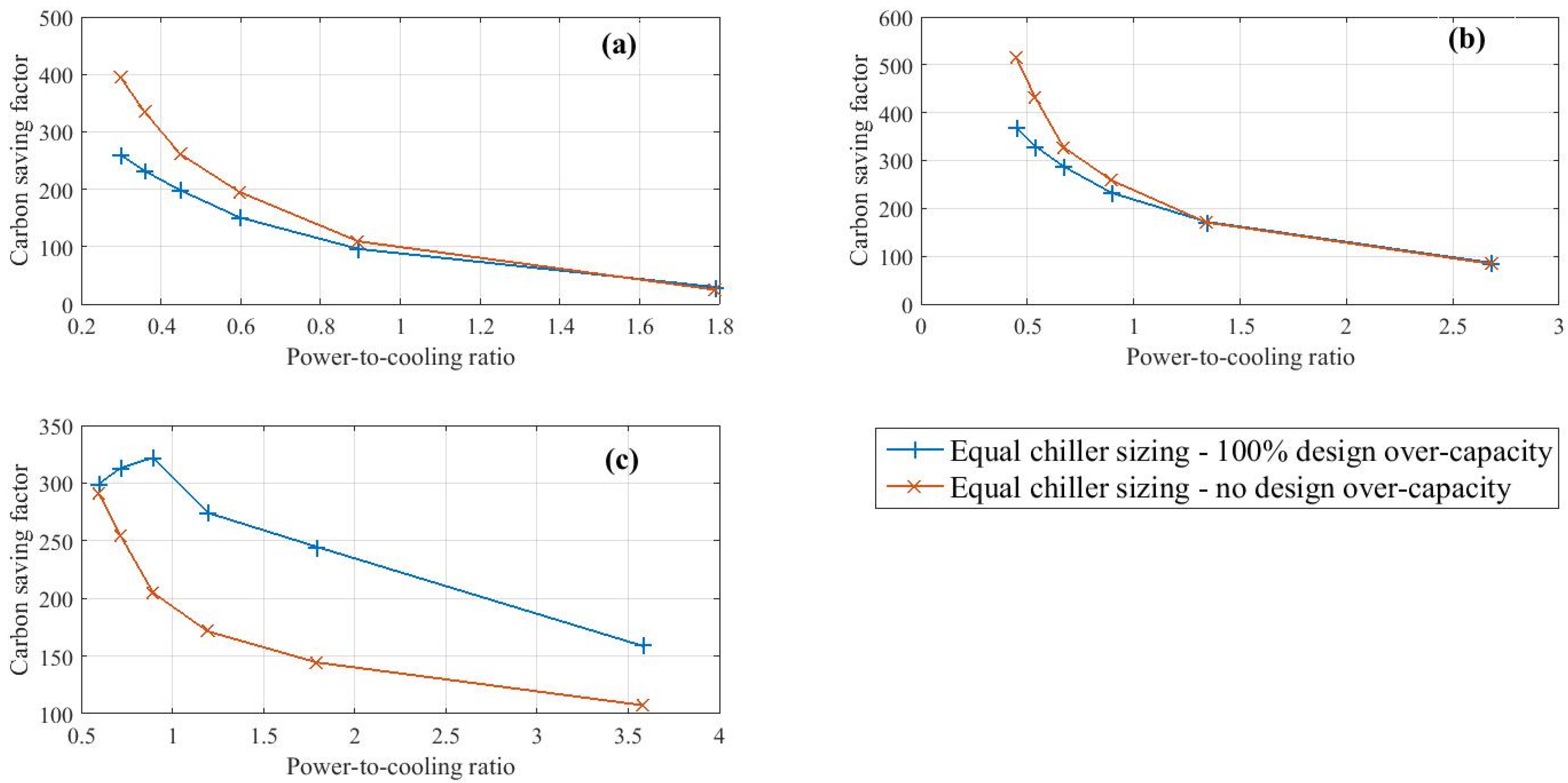
Figure 7.
Maximised carbon factor vs. power-to-cooling ratio. Power demand: (a) 895 kW; (b) 1342.5 kW; (c) 1790 kW.
Figure 7.
Maximised carbon factor vs. power-to-cooling ratio. Power demand: (a) 895 kW; (b) 1342.5 kW; (c) 1790 kW.

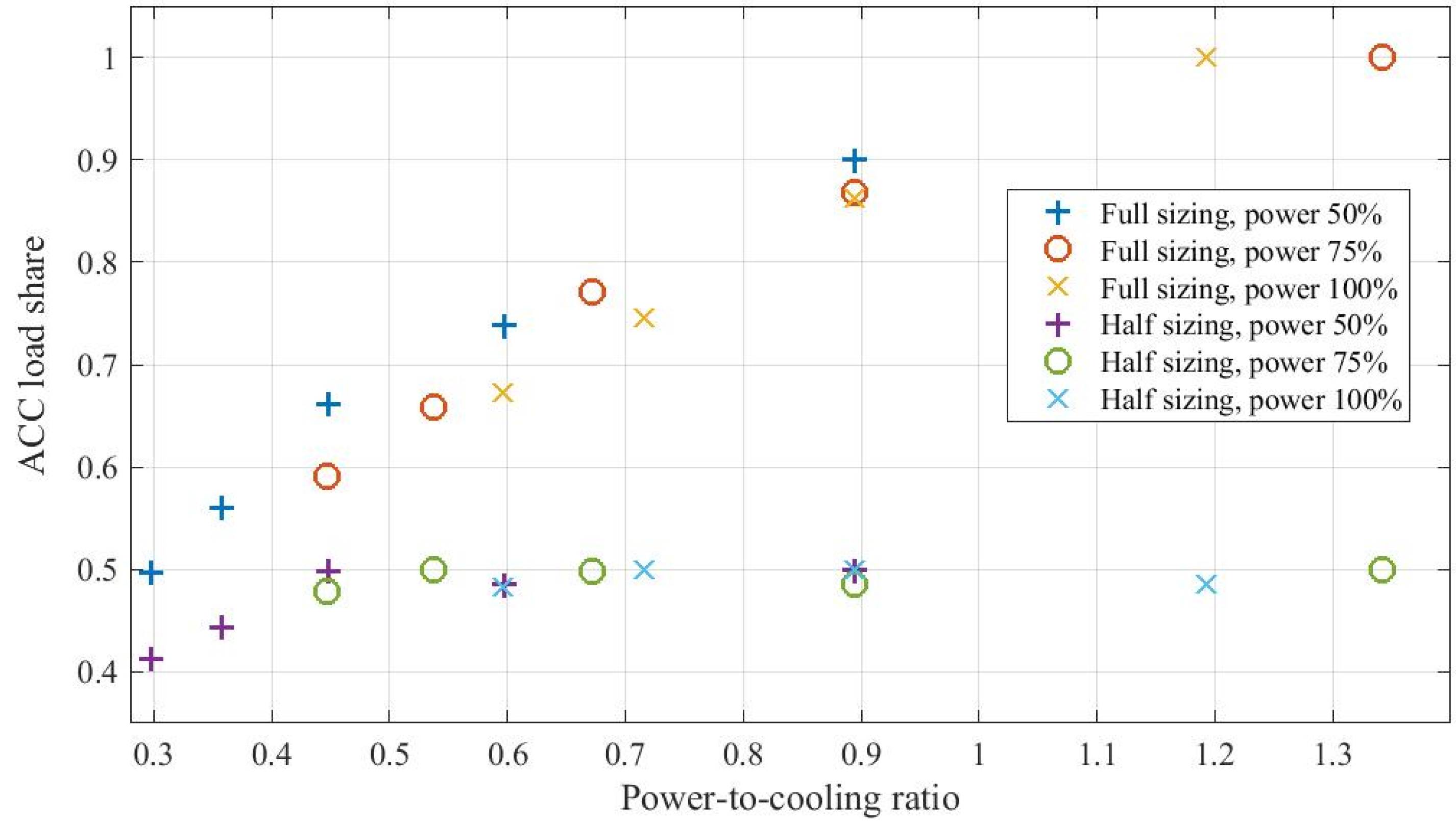
Figure 8.
Share of the cooling load met by the absorption cycle chiller.

5.1 Discussion
Results from both types of cost function minimisation (i.e., money and carbon) present the same broad conclusions (Figure 6 and Figure 7) in that highest savings arise in situations where the power-to-cooling ratio is low and the savings decline as the ratio increases.
The best results arise at very low power-to-cooling ratios when the power demand is moderate (Figure 6b and Figure 7b). In these conditions the absorption cycle chiller and compression chiller share the load (with the dominant share taken by the absorption cycle chiller, Figure 8), all CHP waste heat is utilised, and the increase in power generation prompted by the power required by the compression chiller results in the CHP module operating at higher efficiency.
At lower power demands, there is a small saving advantage when limiting the chiller sizes such that they each meet 50% of the cooling demand but this advantage is reversed at high power demand. The reason for the reversal at high power demand is that the restriction in the absorption cycle chiller size means that a greater share of the load has to be met by the compression chiller but, at high power demand, a proportion of the chiller power has to be imported which reduces savings. This also explains the turning point in the fully-sized performances in Figure 6c and Figure 7c where a rapidly increasing proportion of imported power was observed here as the power-to-cooling ratio falls (i.e., cooling demand increases whilst the power demand is high).
In summary, best results occur when the cooling demand is met by a combination of the absorption cycle chiller and vapour compression cycle chiller in circumstances where the power demand is below the rated capacity of the CHP module. In these circumstances, the transfer of some of the cooling load to the compression chiller causes an increase in CHP module power with a consequential increase in engine efficiency.
6. Conclusions
Trigeneration plants in which the air conditioning load is met by a combination of both absorption cycle and high-efficiency centrifugal vapour compression cycle chillers has been explored in this work. An optimisation algorithm has been developed to find the required operating schedule of the two chiller types when operating together with waste heat from the CHP module (for the absorption cycle chiller) and power from the CHP module (topped up with imported power if necessary) for the compression cycle chiller.
An illustrative case study has been presented to demonstrate the method. Results show that the saving in both operating cost and carbon emission can be maximised when the routine building power demand is less than the rated capacity of the CHP plant and the cooling demand is high. In these conditions the optimisation algorithm shares the load between the two chiller types such that all waste heat is utilised by the absorption cycle chiller but the increased power demand due to the compression chiller results in an increase in the capacity (and, hence efficiency) of the CHP module.
Further work is needed in four areas. Firstly, the exploration of a wider range of operating conditions leading to a robust procedure for the design and sizing of the two chillers. Though the illustrative case study in this work looked at two sizing strategies for the chillers, there are numerous other sizing possibilities. Secondly, there is a need to investigate the performance of plant combinations in the field. This would not be possible at pilot scale because these plants tend to be large and so the identification of potential field installations followed by monitoring and evaluation might be a worthwhile option to pursue. Thirdly, for one such field installation, the development and application of an algorithm similar to that reported here but implemented for real-time control would be beneficial. Finally, the results of this work (and many similar contributions to be found in the literature) are very sensitive to energy prices, tax and other incentives which vary widely from country to country. There is a need to explore common themes among these tariff structures and among blocks of trading nations (e.g., the EU) so that the sensitivity of the economic results for trigeneration plants can be tested more widely.
Author Contributions
Chris Underwood conducted the modelling and generated the results. Bobo Ng carried out the review and advised on the research plan. Francis Yik helped with the modelling of the centrifugal chiller, provided data and advised on the research plan.
Conflicts of Interest
The authors declare no conflict of interest.
List of Symbols
| Symbol | Meaning |
| A | Impeller flow discharge area (m2) |
| ACCshare | Cooling proportion met by absorption cycle chiller (dimensionless) |
| Ap…Cp, Ah…Ch | Power and heat efficiency model fitting coefficients (dimensionless) |
| CF | Cost function (dimensionless) |
| CoP | Coefficient of performance (dimensionless) |
| cp | Specific heat capacity (kJkg-1K-1) |
| D | Impeller diameter (m) |
| E | Electricity demand (kW) |
| F | CHP model fuel energy (kW) |
| F | Zero function heat balance vector (kW) |
| f | Fuel/electricity price ratio (dimensionless) |
| H | CHP plant heat energy and heat demand (kW) |
| h | Enthalpy (kJkg-1) |
| J | Jacobian matrix (dimensionless) |
| kWe, MWe | As energy rate units – the ‘e’ implies electrical power |
| m, m’ | Mass flow rate (kgs-1) – prime superscript denotes design conditions |
| N | Rotational speed (RPS) |
| P | Pressure (Nm-2, bar); fuel/electricity tariff price (money units/kWh) |
| p | Weak solution flow adjustment factor (dimensionless) |
| PLR | Part load ratio (dimensionless) |
| Q | Heat rate (kW) |
| Q | Absorber, condenser heat rate vector (kW) |
| R | Gas constant (kJkg-1K-1) |
| S | Money or carbon saving (currency units or kg) |
| T | Temperature (oC, K) |
| U | Peripheral impeller speed (ms-1) |
| V | Volume flow rate (m3s-1) |
| w | Impeller width at discharge (m) |
| v | Specific volume (m3kg-1) |
| X | Mass concentration (dimensionless or percent) |
| Z | Compressibility factor (dimensionless) |
| β | Impeller angle subtended with respect to horizontal (degree) |
| ΔQ | User-supplied integration interval (kW) |
| ΔX | Concentration differential with solidus state (percent) |
| γ | Index of compression of a perfect gas (dimensionless) |
| η | Efficiency, utilisation (dimensionless) |
| ε | Heat exchanger effectiveness (dimensionless) |
| Subscript | Implication/meaning |
| a | Absorber |
| ac | Air conditioning |
| ACC | Absorption cycle chiller |
| bp | Boiler plant |
| c | Condenser |
| car | Carbon |
| chp | Combined heat and power |
| chw | Chilled water |
| clg | Cooling water |
| com | Compressor |
| crit | Critical (state) |
| dem | Demand (in the context of additional heat) |
| e | Evaporator, electricity (context dependent) |
| f | Fuel |
| g | Generator |
| hw | Heating water |
| hx | Heat exchanger |
| i | Inlet |
| im | Import |
| imp | Impeller |
| loss,fixed | Fixed part of compressor power loss |
| o | Outlet |
| p | Power |
| P | Pressure |
| r | Refrigerant |
| s, ss | Strong solution |
| top | Top-up |
| VCC | Vapour compression chiller |
| w, sw | Weak solution |
Appendix
| Variable | Data | ||||||||
|---|---|---|---|---|---|---|---|---|---|
| Rated capacity (kW) | 250 | 500 | 750 | 1000 | 1250 | 1500 | 2000 | 2500 | 3000 |
| mew (kgs-1) | 12 | 24 | 36 | 51 | 60 | 72 | 96 | 120 | 144 |
| mcw (kgs-1) | 15 | 30 | 45 | 64 | 75 | 90 | 120 | 150 | 180 |
| mhw (kgs-1) | 10 | 20 | 30 | 43 | 50 | 60 | 80 | 100 | 120 |
| msw (kgs-1) | 2.21 | 4.24 | 6.48 | 8.57 | 11.04 | 12.79 | 17.17 | 21.54 | 27.61 |
| Tchw,o (oC) | 7 | ||||||||
| Tclgw,i (oC) | 30 | ||||||||
| Thw,i (oC) | 95 | ||||||||
| ε (all heat exchangers) | 0.75 | ||||||||
| Variable | Data | ||||||||
|---|---|---|---|---|---|---|---|---|---|
| Rated capacity (kW) | 250 | 500 | 750 | 1000 | 1250 | 1500 | 2000 | 2500 | 3000 |
| mew (kgs-1) | 12 | 24 | 36 | 51 | 60 | 72 | 96 | 120 | 144 |
| mcw (kgs-1) | 12 | 24 | 36 | 51 | 60 | 72 | 96 | 120 | 144 |
| D (mm) | 83 | 92 | 99 | 107 | 110.3 | 113.9 | 119.4 | 124.0 | 127.5 |
| Wloss (kW) | 2.5 | 5.5 | 7.5 | 10.0 | 12.5 | 15.0 | 20.0 | 25.0 | 30.0 |
| α | 0.15 | ||||||||
| Rated speed (RPS) | 667 | ||||||||
| w (mm) | 10 | ||||||||
| β (degree) | 130 | ||||||||
| Tchw,o (oC) | 7 | ||||||||
| Tclgw,i (oC) | 30 | ||||||||
| Refrigerant type | R134a | ||||||||
| ε (all heat exchangers) | 0.75 | ||||||||
References
- Moya, M.; Bruno, J.C.; Eguia, P.; Torres, E.; Zamora, I.; Coronas, A. Performance analysis of a trigeneration system based on a micro gas turbine and an air-cooled, indirect fired, ammonia-water absorption chiller. Appl. Energy 2011, 88, 4424–4440. [Google Scholar]
- Ho, J.C.; Chua, K.J.; Chou, S.K. Performance study of a microturbine system for cogeneration application. Renew. Energy 2004, 29, 1121–1133. [Google Scholar] [CrossRef]
- Clausse, M.; Meunier, F.; Coulie, J.; Herail, E. Comparison of adsorption systems using natural gas fired fuel cell as heat source, for residential air conditioning. Int. J. Refri. 2009, 32, 712–719. [Google Scholar] [CrossRef]
- Chua, K.J.; Chou, S.K; Yang, W.M.; Yan, J. Achieving better energy-efficient air conditioning—A review of technologies and strategies. Appl. Energy 2013, 104, 87–104. [Google Scholar] [CrossRef]
- Ryan, W. Driving absorption chillers using heat recovery. ASHRAE J. 2004, 46, S31–S38. [Google Scholar]
- Piacentino, A.; Barbaro, C.; Cardona, F.; Gallea, R.; Cardona, E. A comprehensive tool for efficient design and operation of polygeneration-based energy μgrids serving a cluster of buildings. Part I: Description of the method. Appl. Energy 2013, 111, 1204–1221. [Google Scholar] [CrossRef]
- Piacentino, A.; Barbaro, C. A comprehensive tool for efficient design and operation of polygeneration-based energy μgrids serving a cluster of buildings. Part II: Analysis of the applicative potential. Appl. Energy 2013, 111, 1222–1238. [Google Scholar] [CrossRef]
- Mago, P.; Chamra, L. Analysis and optimization of CCHP systems based on energy, economical, and environmental considerations. Energy Build. 2009, 41, 1099–1106. [Google Scholar] [CrossRef]
- Department of Energy and Climate Change. Table 3.4.1; Quarterly Energy Prices September 2009; Department of Energy and Climate Change: London, UK, 2009; p. 40. [Google Scholar]
- Karmacharya, S.; Putrus, G.; Underwood, C.P.; Mahkamov, K.; McDonald, S.; Alexakis, A. Simulation of energy use in buildings with multiple micro generators. Appl. Therm. Eng. 2014, 581–592. [Google Scholar] [CrossRef]
- Cardona, E.; Piacentino, A. A methodology for sizing a trigeneration plant in Mediterranean areas. Appl. Therm. Eng. 2003, 23, 1665–1680. [Google Scholar] [CrossRef]
- Lozano, M.; Carvalho, M.; Serra, L. Operational strategy and marginal costs in simple trigeneration systems. Energy 2009, 34, 2001–2008. [Google Scholar] [CrossRef]
- Piacentino, A.; Gallea, R.; Cardona, F.; Brano, V.L.; Ciulla, G.; Catrini, P. Optimization of trigeneration systems by mathematical programming: Influence of plant scheme and boundary conditions. Energy Convers. Manag. 2015. [Google Scholar] [CrossRef]
- Chicco, G.; Mancarella, P. Trigeneration primary energy saving evaluation for energy planning and policy development. Energy Policy 2007, 35, 6132–6144. [Google Scholar] [CrossRef]
- Kavvadias, K.; Tosios, A.; Maroulis, Z. Design of a combined heating, cooling and power system: Sizing, operation strategy selection and parametric analysis. Energy Convers. Manag. 2010, 51, 833–845. [Google Scholar] [CrossRef]
- Facci, A.L.; Andreassi, L.; Ubertini, S. Optimisation of CHCP (combined heat power and cooling) systems operations strategy using dynamic programming. Energy 2014, 66, 387–400. [Google Scholar] [CrossRef]
- Kavvadias, K.C.; Maroulis, Z.B. Multi-objective optimisation of a trigeneration plant. Energy Policy 2010, 38, 945–954. [Google Scholar] [CrossRef]
- Kong, X.; Wang, R.; Huang, X. Energy optimization model for a CCHP system with available gas turbines. Appl. Therm. Eng. 2005, 25, 377–391. [Google Scholar] [CrossRef]
- Kong, X.; Wang, R.; Li, Y.; Huang, X. Optimal operation of a micro-combined cooling, heating and power system driven by a gas engine. Energy Convers. Manag. 2009, 50, 530–538. [Google Scholar] [CrossRef]
- Yik, F.W.H.; Lai, J.H.K.; Fong, N.K.; Leung, P.H.M.; Yuen, P.L. A case study on the application of air- and water-cooled oil-free chillers to hospitals in Hong Kong. Build. Serv. Eng. Res. Technol. 2012, 33, 263–279. [Google Scholar] [CrossRef]
- Bourdouxhe, J.-P.; Grodent, M.; Lebrun, J. Reference Guide for Dynamic Models of HVAC Equipment; American Society of Heating, Refrigerating and Air-conditioning Engineers: Atlanta, GA, USA, 1998. [Google Scholar]
- National Institute of Standards and Technology. REFPROP: Reference Fluid Thermodynamic and Transport Properties, Version 7; National Institute of Standards and Technology: Gaithersburg, MD, USA, 2007. [Google Scholar]
- American Society of Heating, Refrigerating and Air Conditioning Engineers (ASHRAE). In Handbook of Fundamentals; American Society of Heating, Refrigerating and Air Conditioning Engineers: Atlanta, GA, USA, 2013; p. 71.
- American Society of Heating, Refrigerating and Air Conditioning Engineers (ASHRAE). In Handbook of Fundamentals; American Society of Heating, Refrigerating and Air Conditioning Engineers: Atlanta, GA, USA, 2013; p. 70.
- Underwood, C.P. Chapter 2; HVAC Control Systems—Modelling, Analysis and Design; E & FN Spon: London, UK, 2002; pp. 52–60. [Google Scholar]
- American Society of Heating, Refrigerating and Air Conditioning Engineers (ASHRAE). In Handbook of Fundamentals; American Society of Heating, Refrigerating and Air Conditioning Engineers: Atlanta, GA, USA, 2013; pp. 17–18.
- Trane Classic Absorption Series (model 294). Available online: http://www.trane.com/download/equipmentpdfs/absprc005en.pdf (accessed on 3 July 2015).
- GE Distributed Power—Jenbacher types 3 and 6 gas engines. Available online: https://www.ge-distributedpower.com/products/power-generation (accessed on 4 July 2015).
- Department of Energy and Climate Change. Table 3.4.1; Quarterly Energy Prices March 2015; Department of Energy and Climate Change: London, UK, 2015; p. 40. [Google Scholar]
- Greenhouse Gas Conversion factor Repository. Available online: http://www.ukconversionfactorscarbonsmart.co.uk/ (accessed on 5 July 2015).
© 2015 by the authors; licensee MDPI, Basel, Switzerland. This article is an open access article distributed under the terms and conditions of the Creative Commons Attribution license (http://creativecommons.org/licenses/by/4.0/).
Share and Cite
MDPI and ACS Style
Underwood, C.; Ng, B.; Yik, F. Scheduling of Multiple Chillers in Trigeneration Plants. Energies 2015, 8, 11095-11119. https://doi.org/10.3390/en81011095
AMA Style
Underwood C, Ng B, Yik F. Scheduling of Multiple Chillers in Trigeneration Plants. Energies. 2015; 8(10):11095-11119. https://doi.org/10.3390/en81011095
Chicago/Turabian StyleUnderwood, Chris, Bobo Ng, and Francis Yik. 2015. "Scheduling of Multiple Chillers in Trigeneration Plants" Energies 8, no. 10: 11095-11119. https://doi.org/10.3390/en81011095