Numerical Analysis on the Optimization of Hydraulic Fracture Networks

Abstract

The clear understanding of hydraulic fracture network complexity and the optimization of fracture network configuration are important to the hydraulic fracturing treatment of shale gas reservoirs. For the prediction of hydraulic fracture network configuration, one of the problems is the accurate representation of natural fractures. In this work, a real natural fracture network is reconstructed from shale samples. Moreover, a virtual fracture system is proposed to simulate the large number of small fractures that are difficult to identify. A numerical model based on the displacement discontinuity method is developed to simulate the fluid-rock coupling system. A dimensionless stress difference that is normalized by rock strength is proposed to quantify the anisotropy of crustal stress. The hydraulic fracturing processes under different stress conditions are simulated. The most complex fracture configurations are obtained when the maximum principle stress direction is perpendicular to the principle natural fracture direction. In contrast, the worst results are obtained when these two directions are parallel to each other. Moreover, the side effects of the unfavorable geological conditions caused by crustal stress anisotropy can be partly suppressed by increasing the viscous effect of the fluid.

1. Introduction

The dense spacing hydraulic fracture network is important for shale gas reservoirs [1,2]. Generally, there are two kinds of factors related to the hydraulic fracturing process. One kind is the geological parameters, such as the rock properties and crustal stress conditions. Another kind is the operating parameters, such as the injection rate and fluid viscosity. Given the geological conditions, it is important to understand how fractures propagate and to find the optimal operating parameters under these geological conditions.

Fracturing treatment designs rely heavily on imprecise estimates of the stimulated reservoir volume derived from micro-seismic observations and through a highly inefficient trial-and-error approach [3]. However, the details of fracture networks cannot be measured by these observation methods. The fracture propagation has also been observed in laboratory [4,5,6]. However, it is difficult to observe fracture network propagation in the laboratory and to know how laboratory experiments relate to the reservoir scale [7]. Compared with the above methods, numerical modelling is much more flexible. Numerical models can be established according to field conditions and all the details can be exported for analysis. Therefore, numerical modeling is an important tool for engineers to predict the geometry of fracture networks [8].

Numerical models should capture all the essential elements so that a simulation reasonably represents the real process [7]. However, the rigorous simulation of all the aspects is very challenging. Many early stage models, such as the PK model [9], PKN model [10], KGD model [11], pseudo-3D models and planar-3D models [12,13], can only be used in simulating the propagation of fractures with highly idealized geometries. Models for the simulation of complex fracture networks are still in development in recent years. These models can roughly be classified into three kinds. The first kind is the models which need grid meshing in the whole region, such as the finite difference method [14], finite element method [15], extended finite element method [16,17,18] and discrete element method [19,20], etc. There are many softwares based on these methods, such as UDEC/3DEC, PFC, RFPA, FLAC, etc. However, while these methods are easy to use, they are far from perfect. As the simulation domain is often several orders bigger than the aperture of fractures, a deformation that is considered as small “noise” in a solid solver may induce dramatic oscillations of fluid pressure in a flow solver [19]. As a result, these methods are ill-conditioned for the fluid-rock coupling system of hydraulic fracturing. Another problem is the complexity of grid re-meshing, which is necessary for the accurate simulation of fracture trajectory [20]. The second kind is meshless methods. Different from traditional methods, meshless methods [21,22,23] are free from meshing and have the capability to deal with moving boundary conditions. Meshless methods are flexible and computationally efficient in simulating fracture propagation, but have not been in used in simulating the complex fracture network propagation in hydraulic fracturing.

The third kind of fracture network simulation model is the models based on Displacement Discontinuity Method (DDM) [24,25,26,27], which is a kind of boundary element method. In DDM-based models, grid meshing is needed only for fractures. The propagation of a fracture network can be simulated within less CPU time because the grid number is far less than in the above models. Fracture aperture can be calculated with higher precision because the stress interaction between fractures is directly calculated by analytical solutions. Moreover, when fractures extend, the grid can be adjusted by simply adding new fracture elements. Based on DDM, Zhang and Jeffrey [28] investigated the injection type on the creation of complex fracture network and it was found that the equal rate injection is better than the equal pressure injection. McClure and Horne [29] simulated the propagation of complex fracture network and showed that fractures may propagate through a mixture of the opening and sliding of preexisting fractures and the propagation of new fractures. Zhang et al. [30] investigated the stability of hydraulic fracture network propagation and found that the localization instability can be suppressed by fluid viscosity. To sum up, the DDM-based models are appropriate for the simulation of complex fracture networks and have been used by more and more researchers [3,7,8,28,29,30,31,32,33].

The Natural Fracture (NF) characterization is also a critical foundation. NFs often lead to the formation of complex fracture geometries by altering the propagating direction of Hydraulic Fracture (HF). However, it’s difficult to obtain the geometry of NFs. For theoretical purposes, idealized NF geometries are acceptable [34], but for engineering purposes, complex fracture networks are required. The Discrete Fracture Network (DFN) model is always used to reconstruct complex NF networks. With the distributions of fracture length, orientation, aperture, etc., and the fracture density, random NF networks can be created [20]. The DFN model has been used by many researchers [3,7,8,20,32]. For example, Riahi and Damjanac [20] investigated the effects of NF connectivity, injection pressure, etc., on the complexity of hydraulic fracture network. Kresse et al. [32] investigated the propagation of fracture networks when complex natural fractures are created. McClure and Horne [7] investigated how shear stimulation can affect the process of fluid propagation. In summary, it’s a useful method to reconstruct the complexity of NF network by random distributions. However, no matter how many distributions are used, the randomly created NF networks are never totally equivalent to the real fracture network.

In this work, the NF network is reconstructed from shale samples. Considering the characteristics of the real NF network, a virtual fracture system is proposed to deal with the small fractures that are difficult to identify from shale samples. A DDM-based numerical model is developed to investigate how hydraulic fracture networks propagate under different stress conditions and how to get complex hydraulic fracture network by adjusting the viscous effect of the fluid.

2. The Model

2.1. Basic Equations

The fluid-rock coupling process of hydraulic fracturing is simulated based on DDM. The following assumptions are used: the domain of the rock matrix is infinite and the rock matrix is homogeneous, isotropous and linearly elastic [35]. The rock matrix is impermeable. The fluid injected is Newtonian, single phase and laminar [7,28,36].

As a kind of boundary element method, the theoretical solution of elastic mechanics [35] is directly used in DDM. Given a fracture system with N fractures, the stress induced by the opening and sliding of these fractures is calculated by [28]:

$$\begin{array}{l}{\sigma }_{\text{n}}\left(x\right)={\displaystyle \sum _{\text{r}=1}^N{\displaystyle {\int }_0^{l_{\text{r}}}\left[G_{11}\left(x,s\right)w\left(s\right)+G_{12}\left(x,s\right)\nu \left(s\right)\right]K\left(x,s\right)\text{d}s}}\\ {\mathrm{\tau }}_{\text{s}}\left(x\right)={\displaystyle \sum _{\text{r}=1}^N{\displaystyle {\int }_0^{l_{\text{r}}}\left[G_{21}\left(x,s\right)w\left(s\right)+G_{22}\left(x,s\right)\nu \left(s\right)\right]K\left(x,s\right)\text{d}s}}\end{array}$$

(1)

where x= (x, y) is the coordinate, w is the normal displacement discontinuity, which equals to the fracture aperture, v is the shear displacement discontinuity, which equals to the sliding distance of fracture surface, l_r is the length of fracture r, G_ij are the hyper singular Green’s functions, which are proportional to the plane strain Young’s modulus [28], σ_n is the normal stress and τ_s is the shear stress, obeying Coulomb’s frictional law characterized by the friction coefficient λ, which limits the shear stress by:

$$\left|{\mathrm{\tau }}_{\text{s}}\right|\le {\mathrm{\lambda }\mathrm{\sigma }}_{\text{n}}$$

(2)

that can act in parts of fractures that are in contact, but vanish along the separated parts. Along the opened fracture portions with fluid pressure p_f, we have:

$${\mathrm{\sigma }}_{\text{n}}=p_{\text{f}}$$

(3)

K is the three dimensional correction coefficient. Using the parameters given by Wu and Olson [37], the correction coefficient K proposed by Olson [38] can be written as:

$$K\left(x_1,x_2\right)=1-\frac{d^3}{{\left[d^2-{\left(h/2\right)}^2\right]}^{3/2}}$$

(4)

where h is the limite layer thickness perpendicular to the simulation plain, d is the distance between points x₁ and x₂.

Volumetric flux q of fluid in fracture is described by:

$$q=-\frac{{\left(w+w_0\right)}^3}{12\mathrm{\mu }}\frac{\partial p_{\text{f}}}{\partial s}$$

(5)

where μ is fluid dynamic viscosity, w₀, which is a reflection of the fracture surface roughness, is the initial hydraulic aperture, w is the aperture, $\frac{\partial p_{\text{f}}}{\partial s}$ is fluid pressure gradient.

The global mass balance requires:

$$\frac{\partial }{\partial t}\left(\frac{\mathrm{\delta }{v}_{\text{f}}}{\mathrm{\delta }L}\right)+\frac{\partial q}{\partial s}=0$$

(6)

where v_f is fluid volume, L is fracture segment length, q is the volumetric flux of fluid.

The fracture growth is based on the maximum hoop stress criterion, with the maximum mixed-mode intensity factor reaching a critical value:

$$\frac{1}{2}\cos \frac{\mathrm{\theta }}{\text{2}}\left[K_{\text{I}}\left(1+\cos \mathrm{\theta }\right)-3K_{\text{II}}\sin \mathrm{\theta }\right]=K_{\text{IC}}$$

(7)

where K_I and K_II are stress intensity factors, K_IC is tensile mode fracture toughness, θ is the fracture propagation direction relative to the current fracture orientation and satisfies:

$$K_{\text{I}}\sin \mathrm{\theta }+K_{\text{II}}\left(3\cos \mathrm{\theta }-1\right)=0$$

(8)

The fractures are meshed with constant displacement elements. The hydraulic fracture problem is solved simultaneously including the effects of viscous fluid flow and coupled rock deformation.

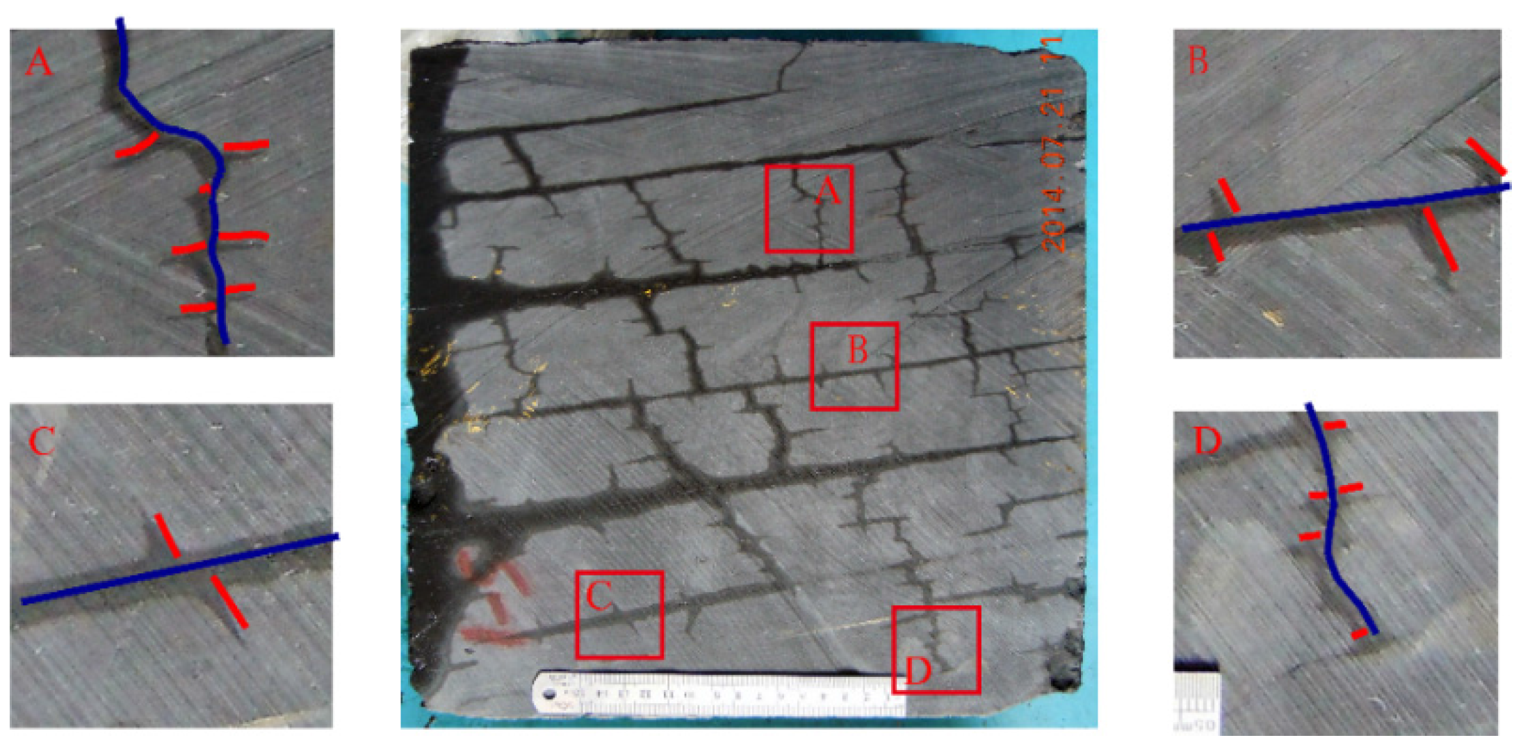
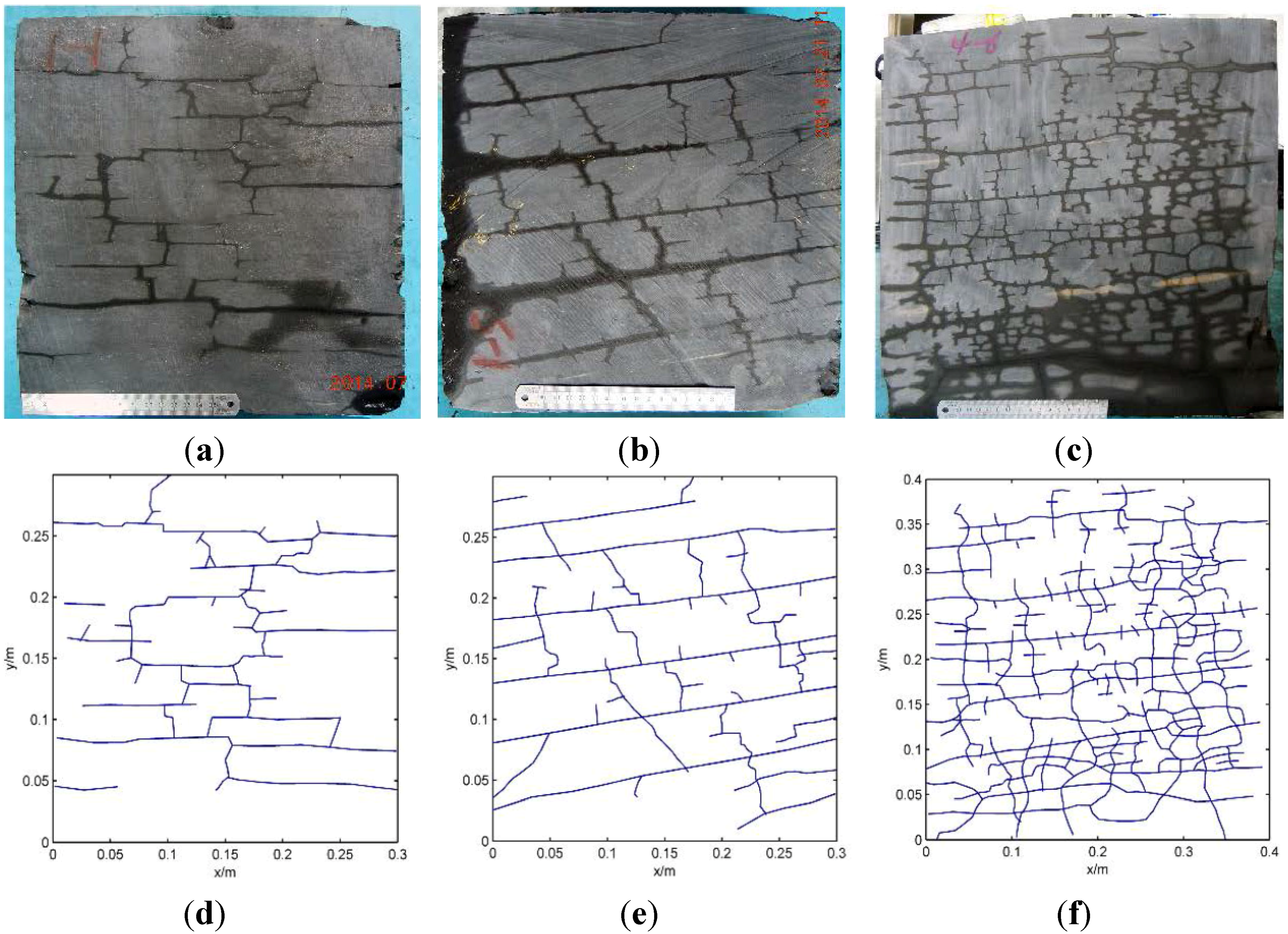
2.2. Natural Fracture Network

NF networks are measured from shale samples, which are sampled from the outcrops of the Longmaxi Formation in South China. As the fracture aperture is always no bigger than 100 μm, it’s impossible to directly obtain the fracture trajectory. Therefore, water was sprinkled over the shale sample. Some water enters NFs so that the rock surface is darker near NFs. The surfaces of the shale samples are shown in Figure 1a–c. The fracture trajectories are identified from the photos to get the data used in modelling. The fracture trajectories are shown in Figure 1d–f.

Figure 1. The natural fracture networks created from the rock sample: (a–c) are the surfaces of the rock sample that wetted by water; (d–f) are the main fractures obtained from the rock sample.

Figure 1. The natural fracture networks created from the rock sample: (a–c) are the surfaces of the rock sample that wetted by water; (d–f) are the main fractures obtained from the rock sample.

Two characteristics are important to our modelling:

(1)

The complete identifying of NF is impossible. By contrast, many small fractures are not clearly shown.

(2)

There are two orthogonal sets of fractures. The length is longer and the connectivity is better for the horizontal set.

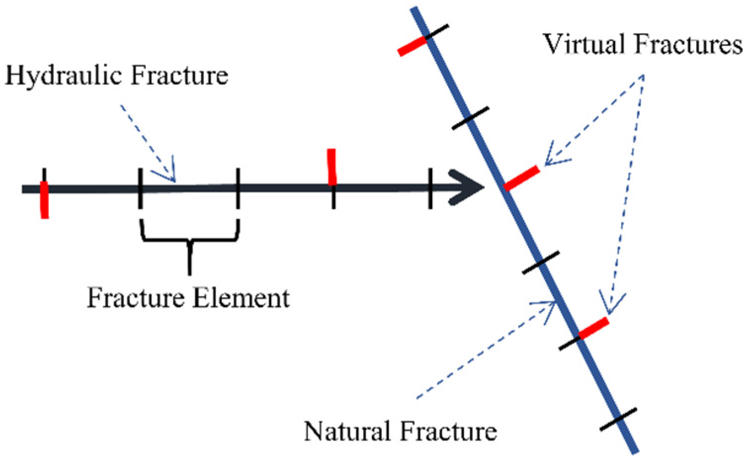
2.3. Virtual Fracture System

There are large number of small fractures that are difficult to be identified. As shown in Figure 2, there are many small fractures that are linked to the main fractures. In fact, there are many other fractures that cannot be seen in the photos. Although the aperture of these fractures is small and the length is short, the strength of these fractures is smaller than the rock matrix. Therefore, the effect of these small fractures is not ignorable.

A virtual fracture system is introduced to simulate these small fractures. First, when a HF encounters a NF, a virtual fracture is added at the other side of the NF. Second, virtual fractures are added randomly to some fracture elements. The methodologies are illustrated in Figure 3. During the simulation, the virtual fractures are checked under the in situ stress conditions. If propagation can occur for a virtual fracture, it means that the in situ stress is so big that the rock may break at the location of the virtual fracture. Under this circumstance, a new fracture element would be added. Otherwise, the small fractures can be treated as if they do not exist and the rock matrix can be treated as homogeneous. This is what the term “virtual” refers to.

Virtual fractures are useful in simulating the creation of complex fracture networks. When virtual fractures extend, new fracture branches are formed and thus the fracture network becomes more complex. The interaction between HF and NF can also be simulated conveniently using the virtual fracture system. The HF will across the NF when the virtual fracture element at the crossing point can extend. Moreover, as no stress is induced by the virtual fractures, no extra computationally demanding is needed. The using of virtual fracture in the modelling will be introduced in Section 2.4.

Figure 2. The small fractures around main fractures.

Figure 2. The small fractures around main fractures.

Figure 3. The setting of virtual fractures. The blue line represents the NF, the black line represents the HF, and the small red lines represent the virtual fracture elements.

Figure 3. The setting of virtual fractures. The blue line represents the NF, the black line represents the HF, and the small red lines represent the virtual fracture elements.

2.4. The Work Flow

The most important process of the modelling is the calculating of p_f, w, v and v_f, where p_f is fluid pressure, w is aperture, v is sliding distance, v_f is fluid volume. A Gauss-Seidel iteration method is used to calculate these values. The balance values of each element are calculated by finding the values which satisfy the Equations (2), (3), (5) and (6). The most time-consuming process is the calculating of in situ stress by Equation (1), which is required for solving these balance values and must be updated in each iteration. As the in situ stress is related to all fractures, the computational demands increase rapidly with the element number. Generally, more than 95% of CPU time is consumed in this process, which is shown as the red dashed box in Figure 4. It must be noted that the virtual fractures are not incorporated in this process. Therefore, although there are large number of virtual fractures, the effectiveness of the solution is not affected.

After p_f, w, v and v_f are updated, the virtual fractures and the ordinary fractures are checked individually to see if fractures could propagate. Specially, for the virtual fractures, as shown in the blue dashed box in Figure 4, we calculate the in situ stress and then the stress intensity factor. If the stress intensity factor is bigger than the fracture toughness, a new ordinary fracture element is added and the corresponding virtual fracture is removed.

Figure 4. The flowchart of the model.

Figure 4. The flowchart of the model.

3. Model Validation

3.1. Against Theoretical Solution

The solving of fracture aperture is a most important foundation. Given the fluid pressure, the profile of the aperture w of a single fracture in infinite rock matrix follows [35]:

$$w\left(x\right)=-\frac{2\left(1-{\nu }_{\text{Po}}\right)}{G}{p}_{\text{f}}a\sqrt{1-\frac{x^2}{a^2}}$$

(9)

where a is the fracture half length, p_f is the net fluid pressure, x is the distance to the center of the fracture, G is the shear modulus, ν_Po is the Poisson’s ratio.

The numerical model is validated against the analytical solution. A single fracture is simulated with the parameters listed in Table 1. The aperture profile of the fracture is compared with the analytical solution as shown in Figure 5. The numerical results agree well with the analytical one, even when there are only ten grids.

The precisely solving of aperture is especially important for the tip element because the intensity factor is calculated by the displacements of the tip element [39]:

$$K_{\text{I}}=\frac{2G}{\kappa +1}w\sqrt{\frac{\mathrm{\pi }}{l}}$$

(10)

$$K_{\text{II}}=\frac{2G}{\kappa +1}v\sqrt{\frac{\mathrm{\pi }}{l}}$$

(11)

where $\mathrm{\kappa }=3-4v_{\text{Po}}$, w and v are the normal and shear displacements of the tip element respectively, l is the length of the tip element.

Table 1. Input parameters for the calculation of fracture aperture profile.

Parameter	Value	Parameter	Value
Fracture length	1 m	Layer thickness	Infinite
$p_{\text{f}}/G$	1	Far-field stress	${\mathrm{\sigma }}_x={\mathrm{\sigma }}_y=0$
Poisson’s ratio	0.1

Table 1. Input parameters for the calculation of fracture aperture profile.

Parameter	Value	Parameter	Value
Fracture length	1 m	Layer thickness	Infinite
$p_{\text{f}}/G$	1	Far-field stress	${\mathrm{\sigma }}_x={\mathrm{\sigma }}_y=0$
Poisson’s ratio	0.1

Figure 5. The comparison of numerical modelling with analytical solution.

Figure 5. The comparison of numerical modelling with analytical solution.

Table 2 shows the precision of the displacements of tip element under different grid numbers. The error of the numerical simulation is significant. The reason is the using of the constant displacement element. Fortunately, the error is almost a constant. As shown in Table 2, the computed aperture is approximately 1.25 times bigger than the analytical value. Therefore, a correction coefficient is introduced, i.e.:

$$K_{\text{I}}=C\frac{2G}{\kappa +1}w\sqrt{\frac{\mathrm{\pi }}{l}}$$

(12)

$$K_{\text{II}}=C\frac{2G}{\kappa +1}v\sqrt{\frac{\mathrm{\pi }}{l}}$$

(13)

where C = 1/1.25 is the correction coefficient.

Table 2. The comparison of numerical modelling with analytical solution for the aperture of tip element. Here x is the coordinate of the center of tip element.

Grid N	(a – x)/L	Numerical (m)	Analytical (m)	Numerical/Analytical
10	0.050	0.498	0.392	1.270
30	0.017	0.290	0.230	1.259
50	0.010	0.225	0.180	1.250
70	0.0071	0.190	0.152	1.250
90	0.0056	0.168	0.134	1.253
100	0.0050	0.159	0.127	1.252

Table 2. The comparison of numerical modelling with analytical solution for the aperture of tip element. Here x is the coordinate of the center of tip element.

Grid N	(a – x)/L	Numerical (m)	Analytical (m)	Numerical/Analytical
10	0.050	0.498	0.392	1.270
30	0.017	0.290	0.230	1.259
50	0.010	0.225	0.180	1.250
70	0.0071	0.190	0.152	1.250
90	0.0056	0.168	0.134	1.253
100	0.0050	0.159	0.127	1.252

3.2. Against Numerical Modelling

We refer for comparison to the model of Wu and Olson [8] for the fracture configurations of a single horizontal wellbore with two initial fractures (Figure 6a) and two horizontal wellbores with one fractures each (Figure 6b). These are the most classic configurations and have been simulated in many works [3,8,32,37,40,41]. The correct simulation of these configurations requires the precisely solving of the stress field and fluid pressure, and the correct calculating of the stress intensity factors of fracture tips. These two configurations are simulated with the parameters listed in Table 3, which is the same to that of Wu and Olson [8]. The results are shown in Figure 7.

Figure 6. Two initiation fractures in (a) a horizontal wellbore and (b) two horizontal wellbores. Blue lines represent horizontal wellbores, and red lines represent initial fractures.

Figure 6. Two initiation fractures in (a) a horizontal wellbore and (b) two horizontal wellbores. Blue lines represent horizontal wellbores, and red lines represent initial fractures.

Figure 7. Comparison of propagation paths for initiation fractures in (a) a horizontal wellbore and (b) two horizontal wellbores. The line width represents the fracture aperture.

Figure 7. Comparison of propagation paths for initiation fractures in (a) a horizontal wellbore and (b) two horizontal wellbores. The line width represents the fracture aperture.

Table 3. Input parameters (Reproduced from Wu and Olson [8]).

Parameter	Value	Parameter	Value
q	8.8 × 10−4 m3/s/m	h	120 m
μ	1.0 cP	KIC	1.0 × 106 Pa.m0.5
E	3.0 × 1010 Pa	Far-field stress	${\mathrm{\sigma }}_x={\mathrm{\sigma }}_y=47 \text{MPa}$
Poisson’s ratio	0.35

Table 3. Input parameters (Reproduced from Wu and Olson [8]).

Parameter	Value	Parameter	Value
q	8.8 × 10−4 m3/s/m	h	120 m
μ	1.0 cP	KIC	1.0 × 106 Pa.m0.5
E	3.0 × 1010 Pa	Far-field stress	${\mathrm{\sigma }}_x={\mathrm{\sigma }}_y=47 \text{MPa}$
Poisson’s ratio	0.35

For the initial configuration as shown in Figure 6a, the two fractures propagate away from each other while for the initial configuration as shown in Figure 6b, the two fractures grow toward each other. In summary, our model compares favorably with previous models.

4. Results and Discussion

4.1. Numerical Setting

As shown in Figure 8, fluid is injected from the center of the region with constant flow rate q_inj. As fluid must be injected in fractures, two small fractures as the red “+” shown in Figure 8 are added. Therefore, the initial fractures may propagate simultaneously along both x and y directions. This is helpful in reducing the influence of initial orientation on final configuration.

The rock matrix is assumed to be infinite. Therefore, no boundary conditions are needed. The maximum principle stress direction of far field stress is represented by ψ. The default input parameters are listed in Table 4, which is used in the following sections if there is no special statement. The simulation is ended when any HF reaches the boundary, i.e., the red dashed box in Figure 8.

Figure 8. The numerical setting.

Figure 8. The numerical setting.

Table 4. The default values of the input parameters.

Parameter	Value	Parameter	Value
q	0.001 m3/s/m	NF aperture	10μm
μ	1 cP	Fracture spacing	0.027 m
E	1.8 × 1010 Pa	ψ	$0°$
Poisson’s ratio	0.18	${\mathrm{\sigma }}_{\text{max}}-{\mathrm{\sigma }}_{\text{min}}$	9 MPa
h	0.3 m	${\mathrm{\sigma }}_{\text{max}}+{\mathrm{\sigma }}_{\text{min}}$	100 MPa
KIC	0.5 × 106 Pa.m0.5	$p_{\text{f}}$ precision $\mathrm{\epsilon }$	1 Pa

Table 4. The default values of the input parameters.

Parameter	Value	Parameter	Value
q	0.001 m3/s/m	NF aperture	10μm
μ	1 cP	Fracture spacing	0.027 m
E	1.8 × 1010 Pa	ψ	$0°$
Poisson’s ratio	0.18	${\mathrm{\sigma }}_{\text{max}}-{\mathrm{\sigma }}_{\text{min}}$	9 MPa
h	0.3 m	${\mathrm{\sigma }}_{\text{max}}+{\mathrm{\sigma }}_{\text{min}}$	100 MPa
KIC	0.5 × 106 Pa.m0.5	$p_{\text{f}}$ precision $\mathrm{\epsilon }$	1 Pa

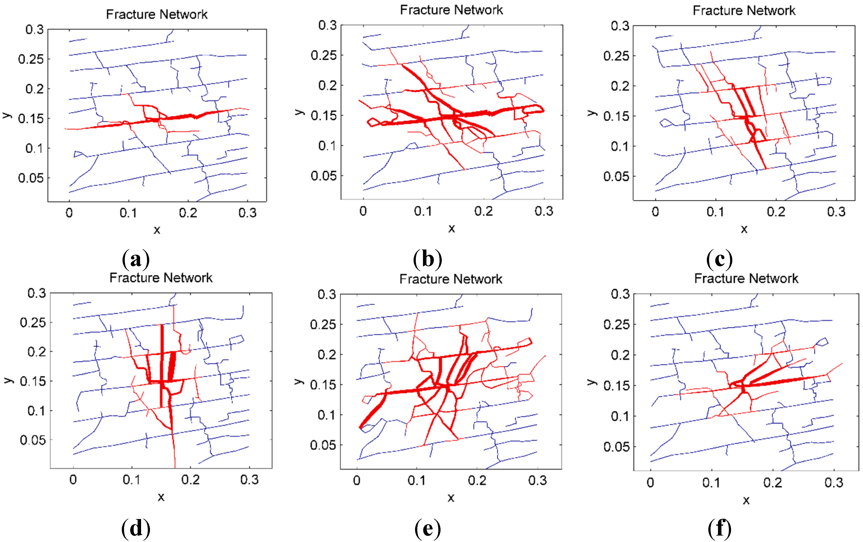
4.2. Quantification of Stress Anisotropy and Fluid Viscosity

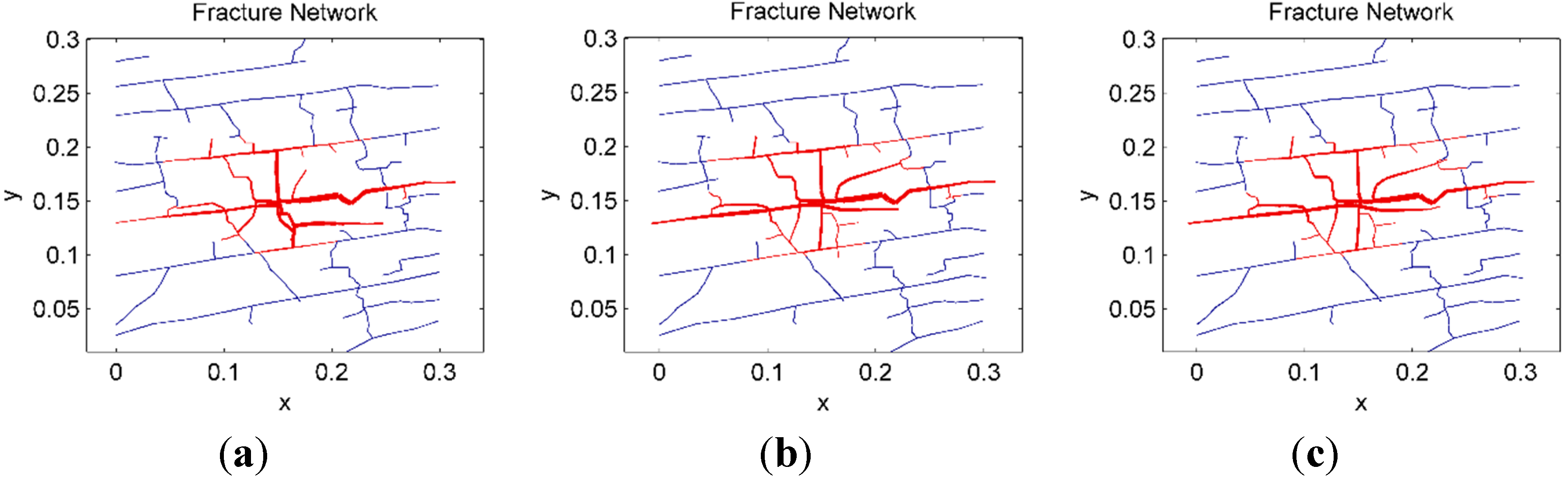
Generally, the stress anisotropy can be quantified by both the stress ratio and stress difference. In this part, we will first check which is more closely related to the propagation of fracture network. The effect of stress ratio is first checked. The fracturing processes under same stress ratio but different stress amplitudes are simulated. The results are shown in Figure 9, which shows different fracture configurations under same stress ratio. By contrast, for the fracturing processes under same stress difference, the final fracture configurations are almost equal as shown in Figure 10. These results indicate that stress difference is better in quantifying the stress anisotropy that related to fracture network configuration.

Figure 9. Fracture configurations under ${\mathrm{\sigma }}_x/{\mathrm{\sigma }}_y=0.8$. The fractures affected by the fluid injection are colored red and other fractures are colored blue: (a) ${\mathrm{\sigma }}_x=10 \text{MPa}$; (b) ${\mathrm{\sigma }}_x=30 \text{MPa}$; (c) ${\mathrm{\sigma }}_x=50 \text{MPa}$.

Figure 9. Fracture configurations under ${\mathrm{\sigma }}_x/{\mathrm{\sigma }}_y=0.8$. The fractures affected by the fluid injection are colored red and other fractures are colored blue: (a) ${\mathrm{\sigma }}_x=10 \text{MPa}$; (b) ${\mathrm{\sigma }}_x=30 \text{MPa}$; (c) ${\mathrm{\sigma }}_x=50 \text{MPa}$.

Figure 10. Fracture configurations under ${\mathrm{\sigma }}_x-{\mathrm{\sigma }}_y=4 \text{MPa}$. The fractures affected by the fluid injection are colored red and other fractures are colored blue: (a) ${\mathrm{\sigma }}_x=10 \text{MPa}$; (b) ${\mathrm{\sigma }}_x=30 \text{MPa}$; (c) ${\mathrm{\sigma }}_x=50 \text{MPa}$.

Figure 10. Fracture configurations under ${\mathrm{\sigma }}_x-{\mathrm{\sigma }}_y=4 \text{MPa}$. The fractures affected by the fluid injection are colored red and other fractures are colored blue: (a) ${\mathrm{\sigma }}_x=10 \text{MPa}$; (b) ${\mathrm{\sigma }}_x=30 \text{MPa}$; (c) ${\mathrm{\sigma }}_x=50 \text{MPa}$.

However, it’s not a good idea to directly use the stress difference to quantify the stress anisotropy because the fracture propagation are related not only to the stress condition, but also to the rock properties. The influence of rock properties can be partly removed by using the dimensionless stress difference which is normalized by rock strength. Considering the initiation fluid pressure $p_{\text{ini}}$ can be used as a characterization of rock strength, the stress difference will be normalized by $p_{\text{ini}}$ in this paper. Here $p_{\text{ini}}$ refers to the fluid pressure above which hydraulic fracture begins to propagate. As discussed by Zhang et al. [30], $p_{\text{ini}}$ is proportional to $K_{\text{IC}}/\sqrt{s}$ , where s is the fracture spacing, then we define:

$$SA=\left({\mathrm{\sigma }}_1-{\mathrm{\sigma }}_2\right)\frac{\sqrt{s}}{K_{\text{IC}}}$$

(14)

where SA is the dimensionless stress difference, ${\mathrm{\sigma }}_1$ and ${\mathrm{\sigma }}_2$ are the two principle stresses, s is the average fracturing spacing of NF network. Specifically, when the principle stress directions are parallel to coordinate axis, the dimensionless stress difference can be written as:

$$S{A}_{xy}=\left({\mathrm{\sigma }}_x-{\mathrm{\sigma }}_y\right)\frac{\sqrt{s}}{K_{\text{IC}}}$$

(15)

where ${\mathrm{\sigma }}_x$ and ${\mathrm{\sigma }}_y$ are the principle stresses along x and y directions respectively.

The viscous effect of fluid is an important operating parameter. Normalized by rock strength, a dimensionless number M is proposed to quantify the viscous effect of fluid by Zhang et al. [30]:

$$M\text{=}\frac{q\mathrm{\mu }{E}^3}{K_{\text{IC}}^4}$$

(16)

where q is flow rate, μ is fluid dynamic viscosity, E is the Young’s modulus.

Although fracture network propagation is related to many factors, including $∆\mathrm{\sigma }$, $K_{\text{IC}}$, q, μ and E, the effects of these factors are not independent. By contrast, the effects of these factors can be represented by two dimensionless numbers, i.e., dimensionless stress anisotropy SA and dimensionless viscous effect M as defined in the Equations (14) and (16).

To check the effectiveness of SA and M, we simulated the fracturing processes under same value of SA and M but different values of $∆\mathrm{\sigma }$, $K_{\text{IC}}$ and μ as listed in Table 5. The simulation results are shown in Figure 11. Although all these parameters are different, the fracture configurations are almost equal as the dimensionless numbers are equal. These results indicate that stress anisotropy and fluid viscosity can be clearly quantified by SA and M, respectively.

Figure 11. Fracture network configurations under same values of M and SA. The fractures affected by the fluid injection are colored red and other fractures are colored blue: (a) ${\mathrm{\sigma }}_x-{\mathrm{\sigma }}_y=1 \text{MPa},\mathrm{\mu }=1 \text{cP},K_{\text{IC}}=0.5$ MPa.m^0.5; (b) ${\mathrm{\sigma }}_x-{\mathrm{\sigma }}_y=3 \text{MPa},$ $\mathrm{\mu }=81 \text{cP},{\text{K}}_{\text{IC}}=1.5$ MPa.m^0.5; (c) ${\mathrm{\sigma }}_x-{\mathrm{\sigma }}_y=5 \text{MPa},\mathrm{\mu }=625 \text{cP},K_{\text{IC}}=2.5$ MPa.m^0.5.

Figure 11. Fracture network configurations under same values of M and SA. The fractures affected by the fluid injection are colored red and other fractures are colored blue: (a) ${\mathrm{\sigma }}_x-{\mathrm{\sigma }}_y=1 \text{MPa},\mathrm{\mu }=1 \text{cP},K_{\text{IC}}=0.5$ MPa.m^0.5; (b) ${\mathrm{\sigma }}_x-{\mathrm{\sigma }}_y=3 \text{MPa},$ $\mathrm{\mu }=81 \text{cP},{\text{K}}_{\text{IC}}=1.5$ MPa.m^0.5; (c) ${\mathrm{\sigma }}_x-{\mathrm{\sigma }}_y=5 \text{MPa},\mathrm{\mu }=625 \text{cP},K_{\text{IC}}=2.5$ MPa.m^0.5.

Table 5. Input parameters.

Parameter	(a)	(b)	(c)
$\left({\mathrm{\sigma }}_x-{\mathrm{\sigma }}_y\right)/\text{Pa}$	1.0 × 106	3.0 × 106	5.0 × 106
$\mathrm{\mu }/\text{cP}$	1	81	625
$K_{IC}/\text{Pa}.{\text{m}}^{0.5}$	0.5 × 106	1.5 × 106	2.5 × 106
Fracture spacing/m	0.027	0.027	0.027
M	93.3	93.3	93.3
SAxy	0.33	0.33	0.33

Table 5. Input parameters.

Parameter	(a)	(b)	(c)
$\left({\mathrm{\sigma }}_x-{\mathrm{\sigma }}_y\right)/\text{Pa}$	1.0 × 106	3.0 × 106	5.0 × 106
$\mathrm{\mu }/\text{cP}$	1	81	625
$K_{IC}/\text{Pa}.{\text{m}}^{0.5}$	0.5 × 106	1.5 × 106	2.5 × 106
Fracture spacing/m	0.027	0.027	0.027
M	93.3	93.3	93.3
SAxy	0.33	0.33	0.33

4.3. Effect of Stress Anisotropy

First, we simulated the fracturing processes under different stress differences. All the other parameters are equal and are listed in Table 4. The results are shown in Figure 12. It’s clear that stress difference has significant effect on fracture configuration. When $S{A}_{xy}=3.3$, i.e., the maximum principle stress direction is parallel to x axis, HF propagates mainly along x axis. With the increase of ${\mathrm{\sigma }}_y$, the propagation distance along y axis increases. Thus, the fracture network is more complex and the affected area is bigger when ${\mathrm{\sigma }}_y$ is bigger. The most complex fracture network is obtained when $S{A}_{xy}=-0.66$, under which circumstance the propagation is dominated by two opposite mechanisms. First, fractures tend to propagates along the principle NF direction, which is roughly parallel to x axis. Second, fractures tend to propagate along the maximum principle stress direction, which is parallel to y axis. The optimal results are obtained when the two opposite mechanisms are balanced by each other.

Figure 12. The final fracture networks. The fractures affected by the fluid injection are colored red and other fractures are colored blue: (a) ${\mathrm{\sigma }}_x-{\mathrm{\sigma }}_y=-10 \text{MPa}$, $S{A}_{xy}=-3.3$; (b) ${\mathrm{\sigma }}_x-{\mathrm{\sigma }}_y=-6\text{ MPa}$, $S{A}_{xy}=-2.0$; (c) ${\mathrm{\sigma }}_x-{\mathrm{\sigma }}_y=-2 \text{MPa}$, $S{A}_{xy}=-0.66$; (d) ${\mathrm{\sigma }}_x-{\sigma }_y=2\text{ MPa}$, $S{A}_{xy}=0.66$; (e) ${\mathrm{\sigma }}_x-{\mathrm{\sigma }}_y=6 \text{MPa}$, $S{A}_{xy}=2.0$; (f) ${\mathrm{\sigma }}_x-{\mathrm{\sigma }}_y=10 \text{MPa}$, $S{A}_{xy}=3.3$.

Figure 12. The final fracture networks. The fractures affected by the fluid injection are colored red and other fractures are colored blue: (a) ${\mathrm{\sigma }}_x-{\mathrm{\sigma }}_y=-10 \text{MPa}$, $S{A}_{xy}=-3.3$; (b) ${\mathrm{\sigma }}_x-{\mathrm{\sigma }}_y=-6\text{ MPa}$, $S{A}_{xy}=-2.0$; (c) ${\mathrm{\sigma }}_x-{\mathrm{\sigma }}_y=-2 \text{MPa}$, $S{A}_{xy}=-0.66$; (d) ${\mathrm{\sigma }}_x-{\sigma }_y=2\text{ MPa}$, $S{A}_{xy}=0.66$; (e) ${\mathrm{\sigma }}_x-{\mathrm{\sigma }}_y=6 \text{MPa}$, $S{A}_{xy}=2.0$; (f) ${\mathrm{\sigma }}_x-{\mathrm{\sigma }}_y=10 \text{MPa}$, $S{A}_{xy}=3.3$.

Second, the fracturing processes under different values of $\mathrm{\psi }$ are simulated, where $\mathrm{\psi }$ is the angle between maximum principle stress direction and the positive direction of x axis as shown in Figure 8. $∆\mathrm{\sigma }={\mathrm{\sigma }}_{\text{max}}-{\mathrm{\sigma }}_{\text{min}}=9 \text{MPa}$ is used in the simulation. All the other parameters for these simulations are equal and are listed in Table 4. The simulation results are shown in Figure 13. The fracture configurations vary significantly with $\mathrm{\psi }$. The propagation distance is further along the maximum principle stress direction. This is favorable for the creation of complex fracture network when the maximum principle stress direction is orthogonal to the principle NF direction.

The affected area is exported to investigate how stress anisotropy affects the fracturing result. The affected area is defined as the area of the region which has experienced a fluid pressure incensement due to the fluid injection [20]. Specifically, a fracture is treated as affected when the fluid pressure incensement is bigger than 0.1 MPa in this paper. The variation of affected area with ψ and SA are shown in Figure 14. The affected area decreases with the increasing of SA and reaches its maximum value when the maximum principle stress direction is orthogonal to the principle NF direction.

Figure 13. The fracture network configurations. The fractures affected by the fluid injection are colored red and other fractures are colored blue. (a) $\mathrm{\psi }=0°$; (b) $\mathrm{\psi }=30°$; (c) $\mathrm{\psi }=60°$; (d) $\mathrm{\psi }=90°$; (e) $\mathrm{\psi }=120°$; (f) $\mathrm{\psi }=150°$.

Figure 13. The fracture network configurations. The fractures affected by the fluid injection are colored red and other fractures are colored blue. (a) $\mathrm{\psi }=0°$; (b) $\mathrm{\psi }=30°$; (c) $\mathrm{\psi }=60°$; (d) $\mathrm{\psi }=90°$; (e) $\mathrm{\psi }=120°$; (f) $\mathrm{\psi }=150°$.

Figure 14. The variation of affected area with $\mathrm{\psi }$ and SA. The result of each simulation is represented by a black point. The smoothed value is represented by the colored surface.

Figure 14. The variation of affected area with $\mathrm{\psi }$ and SA. The result of each simulation is represented by a black point. The smoothed value is represented by the colored surface.

The variation of the average sliding distance of fracture in affected region with ψ and SA is shown in Figure 15. As the sliding of a fracture is caused by the shear stress along the fracture, the sliding distance vary significantly with the crustal stress direction. The sliding distance reaches its maximum value when ψ $\approx 45°$, when the shear stress reaches the maximum value. However, the variation of sliding distance with $\mathrm{\psi }$ is significant only when the value of SA is big. Otherwise, if SA is very small, the sliding is also caused by the induced stress of other fractures, which never vary with the stress direction.

Figure 15. The variation of shear displacements with ψ and SA. The result of each simulation is represented by a black point. The smoothed value is represented by the colored surface.

Figure 15. The variation of shear displacements with ψ and SA. The result of each simulation is represented by a black point. The smoothed value is represented by the colored surface.

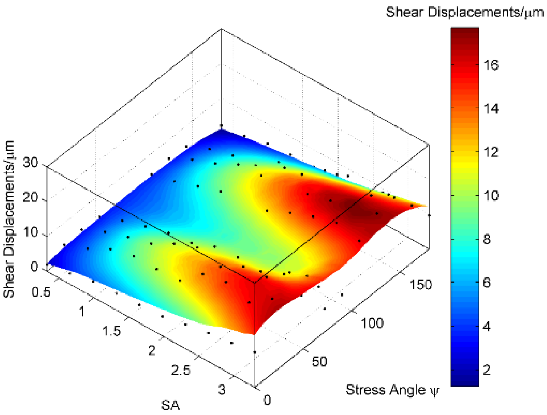
4.4. Effect of Fluid Viscosity

From the analysis of last section, we know the stress anisotropy has significant effect on the fracture network configuration. The problem is, it’s hard to alter the stress condition during fracturing operation. Therefore, when the stress condition is unfavorable for fracturing treatment, the method to reduce the influence of stress anisotropy is very important. As the viscous effect of fluid is one of the most important operating parameters during fracturing treatment, the variation of affected area with SA and M is investigated.

The fracture network propagation under different values of SA and M are simulated. The value of SA is set by adjusting the value of $∆\mathrm{\sigma }={\mathrm{\sigma }}_x-{\mathrm{\sigma }}_y$, the value of M is set by adjusting μ. All the other parameters are listed in Table 4. The affected area is plotted against SA and M in Figure 16, which shows a very clear tendency. When the injection rate is very low or viscous coefficient is small, i.e., the value of M is small, the fracturing result is good only when $S{A}_{xy}\approx -0.6$. By contrast, the optimal fracturing result can be obtained in a wider range of SA_xy when the value of M is bigger. As the dimensionless number M is proportional to both q and μ, these results indicate that, if the crustal stress condition is unfavorable for fracturing treatment, the influence of stress anisotropy can be partly suppressed by increasing the injection rate or fluid viscosity.

Figure 16. The variation of affected area with SA and M. The result of each simulation is represented by a black point. The affected area smoothed from the data points is represented by the colored surface.

Figure 16. The variation of affected area with SA and M. The result of each simulation is represented by a black point. The affected area smoothed from the data points is represented by the colored surface.

5. Conclusions

A natural fracture network can be well represented by identifying the fracture trajectory directly from rock samples along with a virtual fracture system. The virtual fracture system is necessary because it’s impossible to get all the details of NFs. The propagation of virtual fracture can be conveniently simulated within the framework of DDM without the loss of computational efficiency. The virtual fracture system is useful in simulating the HF-NF interactions and is instructive to other numerical methods.

The stress anisotropy can be quantified by defining a dimensionless stress difference SA, which is normalized by the strength of rock matrix. Given the certain value of SA and M, the fracture network has a certain configuration, which is not related to the injection rate, fluid viscosity, stress difference, rock strength, etc.

The propagation direction is dominated mainly by two mechanisms: the NFs and stress condition. As fractures tend to propagate along NFs and the direction of maximum principle stress, the complex fracture network can be formed when these two directions are orthogonal to each other and are balanced by each other. Under this circumstance, the leading propagation direction of HF is not exist. The key point of creating complex fracture network is the eliminating of the leading direction of HF propagation.

The side effect of stress anisotropy on the formation of complex fracture network can be weakened by increasing the viscous effect of fluid. Therefore, if the stress condition is unfavorable to fracturing operation, it is better to increase the injection rate or fluid viscosity.

References

1. Frantz, J.; Jochen, V. Shale gas white paper. Available online: http://www.docin.com/p-364125972.html?qq-pf-to=pcqq.c2c (accessed on 22 October 2015).
2. Harper, J. The marcellus shale—An old “new” gas reservoir in Pennsylvania. Pa. Geol. 2008, 28, 2–13. [Google Scholar]
3. Weng, X. Modeling of complex hydraulic fractures in naturally fractured formation. J. Unconv. Oil Gas Resour. 2015, 9, 114–135. [Google Scholar]
4. Meng, Q.M.; Zhang, S.C.; Guo, X.M.; Chen, X.H.; Zhang, Y. A primary investigation on propagation mechanism for hydraulic fracture in glutenite formation. J. Oil Gas Tech. 2010, 32, 119–123. [Google Scholar]
5. Bunger, A.P.; Gordeliy, E.; Detournay, E. Comparison between laboratory experiments and coupled simulations of saucer-shaped hydraulic fractures in homogeneous brittle-elastic solids. J. Mech. Phys. Solids 2013, 61, 1636–1654. [Google Scholar] [CrossRef]
6. Huang, H.; Zhang, F.; Callahan, P.; Ayoub, J.A. Fluid injection experiments in 2d porous media. SPE J. 2012, 17, 903–911. [Google Scholar] [CrossRef]
7. McClure, M.; Horne, R. Characterizing hydraulic fracturing with a tendency-for-shear-stimulation test. SPE Reserv. Eval. Eng. 2014, 17, 233–243. [Google Scholar] [CrossRef]
8. Wu, K.; Olson, J.E. Simultaneous multifracture treatments: Fully coupled fluid flow and fracture mechanics for horizontal wells. SPE J. 2014, 20, 337–346. [Google Scholar] [CrossRef]
9. Perkins, T.K.; Kern, L.R. Widths of hydraulic fractures. J. Pet. Technol. 1961, 13, 937–949. [Google Scholar] [CrossRef]
10. Nordgren, R.P. Propagation of a vertical hydraulic fracture. Soc. Pet. Eng. J. 1972, 12, 306–314. [Google Scholar] [CrossRef]
11. Geertsma, J.; De Klerk, F. Rapid method of predicting width and extent of hydraulically induced fractures. J. Pet. Technol. 1969, 21, 1571–1581. [Google Scholar] [CrossRef]
12. Advani, S.H.; Lee, T.S.; Lee, J.K. Three-dimensional modeling of hydraulic fractures in layered media: Part I—Finite element formulations. J. Energy Resour. Technol. 1990, 112. [Google Scholar] [CrossRef]
13. Siebrits, E.; Peirce, A.P. An efficient multi-layer planar 3d fracture growth algorithm using a fixed mesh approach. Int. J. Numer. Method Eng. 2002, 53, 691–717. [Google Scholar] [CrossRef]
14. Nagel, N.B.; Sanchez-Nagel, M. Stress shadowing and microseismic events: A numerical evaluation. In Proceedings of the SPE Annual Technical Conference and Exhibition, Denver, CO, USA, 30 October–2 November 2011.
15. Rahman, M.M.; Rahman, S.S. Studies of hydraulic fracture-propagation behavior in presence of natural fractures: Fully coupled fractured-reservoir modeling in poroelastic environments. Int. J. Geomech. 2013, 13, 809–826. [Google Scholar] [CrossRef]
16. Liu, F.S.; Borja, R.I. Extended finite element framework for fault rupture dynamics including bulk plasticity. Int. J. Numer. Anal. Methods Geomech. 2013, 37, 3087–3111. [Google Scholar] [CrossRef]
17. Mohammadnejad, T.; Khoei, A.R. An extended finite element method for fluid flow in partially saturated porous media with weak discontinuities; the convergence analysis of local enrichment strategies. Comput. Mech. 2013, 51, 327–345. [Google Scholar] [CrossRef]
18. Gordeliy, E.; Peirce, A. Coupling schemes for modeling hydraulic fracture propagation using the XFEM. Compu. Methods Appl. Mech. Eng. 2013, 253, 305–322. [Google Scholar] [CrossRef]
19. Fu, P.C.; Johnson, S.M.; Carrigan, C.R. An explicitly coupled hydro-geomechanical model for simulating hydraulic fracturing in arbitrary discrete fracture networks. Int. J. Numer. Anal. Methods Geomech. 2013, 37, 2278–2300. [Google Scholar] [CrossRef]
20. Riahi, A.; Damjanac, B. Numerical study of interaction between hydraulic fracture and discrete fracture network. In Proceedings of the ISRM International Conference for Effective and Sustainable Hydraulic Fracturing, Brisbane, Australia, 20–22 May 2013.
21. Zhuang, X.; Augarde, C.E.; Mathisen, K. Fracture modeling using meshless methods and level sets in 3d: Framework and modeling. Int. J. Numer. Methods Eng. 2012, 92, 969–998. [Google Scholar] [CrossRef]
22. Zhuang, X.; Huang, R.; Liang, C.; Rabczuk, T. A coupled thermo-hydro-mechanical model of jointed hard rock for compressed air energy storage. Math. Probl. Eng. 2014, 2014. [Google Scholar] [CrossRef]
23. Rabczuk, T.; Belytschko, T. Cracking particles: A simplified meshfree method for arbitrary evolving cracks. Int. J. Numer. Methods Eng. 2004, 61, 2316–2343. [Google Scholar] [CrossRef]
24. Li, H.; Liu, C.L.; Mizuta, Y.; Kayupov, M.A. Crack edge element of three-dimensional displacement discontinuity method with boundary division into triangular leaf elements. Int. J. Numer. Methods Biomed. 2001, 17, 365–378. [Google Scholar] [CrossRef]
25. Yan, X.Q.; Liu, B.L. Fatigue growth modeling of cracks emanating from a circular hole in infinite plate. Meccanica 2012, 47, 221–233. [Google Scholar] [CrossRef]
26. Birgisson, B.; Wang, J.L.; Roque, R.; Sangpetngam, B. Numerical implementation of a strain energy-based fracture model for HMA materials. Road Mater. Pavement Des. 2007, 8, 7–45. [Google Scholar] [CrossRef]
27. Dong, C.Y.; Lo, S.H.; Cheung, Y.K. Numerical analysis of the inclusion-crack interactions using an integral equation. Comput. Mech. 2003, 30, 119–130. [Google Scholar] [CrossRef]
28. Zhang, X.; Jeffrey, R. Development of fracture networks through hydraulic fracture growth in naturally fractured reservoirs. In Proceedings of the ISRM International Conference for Effective and Sustainable Hydraulic Fracturing, Brisbane, Australia, 20–22 May 2013.
29. McClure, M.W.; Horne, R.N. Conditions required for shear stimulation in EGS. In Proceedings of the European Geothermal Conference, Pisa, Italy, 3–7 June 2013.
30. Zhang, Z.; Li, X.; He, J.; Wu, Y.; Zhang, B. Numerical analysis on the stability of hydraulic fracture propagation. Energies 2015, 8, 9860–9877. [Google Scholar] [CrossRef]
31. Olson, J.E. Multi-fracture propagation modeling: Applications to hydraulic fracturing in shales and tight gas sands. In Proceedings of the U.S. Rock Mechanics Symposium (USRMS), San Francisco, CA, USA, 29 June–2 July 2008.
32. Kresse, O.; Weng, X.W.; Gu, H.R.; Wu, R.T. Numerical modeling of hydraulic fractures interaction in complex naturally fractured formations. Rock Mech. Rock Eng. 2013, 46, 555–568. [Google Scholar] [CrossRef]
33. McClure, M.W.; Horne, R.N. Discrete Fracture Network Modeling of Hydraulic Stimulation: Coupling Flow and Geomechanics; SpringerBriefs in Earth Sciences, Springer International Publishing: London, UK, 2013. [Google Scholar]
34. Zhang, X.; Jeffrey, R.G. Fluid-driven multiple fracture growth from a permeable bedding plane intersected by an ascending hydraulic fracture. J. Geophys. Res. Solid Earth 2012, 117. [Google Scholar] [CrossRef]
35. Crouch, S.L.; Starfield, A.M. Boundary Element Methods in Solid Mechanics; George Allen & Unwin: London, UK, 1983. [Google Scholar]
36. Weng, X.; Kresse, O.; Cohen, C.; Wu, R.; Gu, H. Modeling of hydraulic-fracture-network propagation in a naturally fractured formation. SPE Product. Oper. 2011, 26, 368–380. [Google Scholar] [CrossRef]
37. Wu, K.; Olson, J.E. Investigation of the impact of fracture spacing and fluid properties for interfering simultaneously or sequentially generated hydraulic fractures. SPE Product. Oper. 2013, 28, 427–436. [Google Scholar] [CrossRef]
38. Olson, J.E. Predicting fracture swarms—The influence of subcritical crackgrowth and the crack-tip process zone on joint spacing in rock. In The Initiation, Propagation, and Arrest of Joints and Other Fractures; Geological Society of London Special Publication: London, UK, 2004; Volume 231, pp. 73–87. [Google Scholar]
39. De, X.; Qin, Q.; Changan, L. Numerical Method and Engineering Application of Fracture Mechanics; Science Press: Beijing, China, 2009. (In Chinese) [Google Scholar]
40. Kresse, O.; Cohen, C.; Weng, X.; Wu, R.; Gu, H. Numerical modeling of hydraulic fracturing in naturally fractured formations. In Proceedings of the 45th US Rock Mechanics/Geomechanics Symposium, San Francisco, CA, USA, 26–29 June 2011.
41. Nagel, N.B.; Gil, I.; Sanchez-nagel, M.; Damjanac, B. Simulating hydraulic fracturing in real fractured rocks—overcoming the limits of pseudo3d models. In Proceedings of the SPE Hydraulic Fracturing Technology Conference, The Woodlands, TX, USA, 24–26 January 2011.