Methodologies and Advancements in the Calibration of Building Energy Models

Abstract

Buildings do not usually perform during operation as well as predicted during the design stage. Disagreement between simulated and metered energy consumption represents a common issue in building simulation. For this reason, the calibration of building simulation models is of growing interest. Sensitivity and uncertainty analyses play an important role in building model accuracy. They can be used to identify the building model parameters most influent on the energy consumption. Given this, these analyses should be integrated within calibration methodologies and applications for tuning the parameters. This paper aims at providing a picture of the state of the art of calibration methodologies in the domain of building energy performance assessment. First, the most common methodologies for calibration are presented, emphasizing criticalities and gaps that can be faced. In particular the main issues to be addressed, when carrying out calibrated simulation, are discussed. The standard statistical criteria for considering the building models calibrated and for evaluating their goodness-of-fit are also presented. Second, the commonly used techniques for investigating uncertainties in building models are reviewed. Third, a review of the latest main studies in the calibrated simulation domain is presented. Criticalities and recommendations for new studies are finally provided.

1. Introduction

Since the mid-1970s, building simulation (BS) has emerged as an attempt to emulate reality [1] and improve on traditional manual methods to study and optimize the energy performance of buildings and systems. At first, BS was used throughout the design process, from the early stages to detailed construction phases. As Clarke pointed out [1], simulation may be used at any design stage to address relevant questions when assisting the building design practice. So far, the BS domain has grown and continuous improvements are being made to software features and, above all, to the building models robustness [2]. In response to current high and ambitious sustainability goals, building design has been recently subjected to changes, involving BS directly. As the main focus is still to reduce the energy demand of the building and optimize its energy performance, BS, as a clear response, is of growing importance. However, its potential is not fully exploited and even acknowledging the upward slope of its productivity for the last two decades, its uptake is still restricted [2]. It is much more common to see BS applications in construction or advanced design phases rather than in early phases (e.g., concept design). Despite this, a recent boost has been given to BS by its application in post-construction stages [3]. Buildings do not perform as well as predicted. Several studies have thus highlighted great discrepancies between simulated building energy performance and measured performance [3,4,5]. Due to this, an extensive interest in building real-monitoring and operation diagnostic has been aroused and the disagreement between measured and simulated data has thus become a primary issue in the BS domain. In order to make BS a more reliable tool for the design process, improvements towards a better match of the simulated and monitored building energy performance have emerged as an imminent need.

This particular application of building simulation is customarily called calibrated simulation (CS). It corresponds to the process of fine-tuning or of “calibrating” the simulation inputs so that the observed energy consumptions closely match those predicted by the simulation program [6]. The use of CS is growing in importance and many activities [3], mostly related to the commissioning or the assessment of the energy retrofit scenario of existing buildings, in fact require a calibration-based study. In particular, on-going and post-construction commissioning of new and existing buildings requires the use of calibrated simulation for operational optimization of control strategies or for diagnostic purposes for further prediction of energy savings [7,8,9].

Additionally, CS has been officially endorsed by the International Performance Measurements and Verification protocol (IPMVP) [10]. Within IPMVP two main approaches for energy savings projects are listed; retrofit isolation options (Option A and B) and whole facility options (Option C and D) [10]. Option D is a simulation-based approach that requires models to be calibrated based on measured monthly or hourly data. CS, within Option D, is the suggested procedure for performance and usage verification of the whole building or specific building components. The IMPVP approach is also applied in the Federal Energy Management Program (FEMP) Measurements and Verification (M&V) guidelines [11].

However, although many improvements have been made in BS and the use of CS is growing fast, many issues and criticalities still characterize the calibration process. When performing CS, it is important to distinguish different levels of calibration. First, depending on the monitored data available, calibration can be performed hourly, or monthly. Second, the type of in-depth analysis on the building model can regard only the building system or the whole building, also described within M&V guidelines [10].

Several studies based on calibration have been carried out [6,12,13,14,15,16,17] but as yet no universal consensus guidelines have been presented. There are thus standard criteria for validating a calibrated model but the lack of a formal and recognized methodology still makes CS a process highly dependent on the user’s skills and judgments.

This paper aims at providing a review of the state of the art in the domain of calibrated simulation. In particular it reviews the current techniques used for calibrating a building model, focusing on gaps and criticalities related to CS. The paper is organized as follows: the scope and applications of CS is given in the introduction; Section 2 briefly outlines the main issues faced when calibrating a building model; Section 3 presents the statistical criteria used for judging the goodness-of-fit of the calibrated models; Section 4 reviews the most used calibration techniques in building simulation domain; Section 5 focuses on the reliability of building models and presents the techniques for investigating uncertainties; Section 6 and Section 7, respectively, provide a brief description of the main CS applications and point out criticalities and gaps in CS.

2. Typical Calibration Issues

Building energy models are complex and composed of a large number of input data. When modeling a building within a simulation program, the accuracy especially relies on the ability of the user to input the parameters (input data) that results in a good model of the actual building energy use [3]. Given the large number of parameters involved, the process of calibrating a detailed energy model is a highly undetermined problem that brings to a non-unique solution [15,18].

It is quite common to use a “trial and error” method to calibrate a building model. This kind of approach, driven by experience assumptions, may bring inexperienced users to time consuming and unsolved problems. Usually building energy models are complex. Many assumptions on the building characterization, with a direct impact on the simulation results, have to be made. Moreover the process of modeling acquires higher degree of difficulty during calibration. Therefore, in order to handle properly the model complexity during calibration, the tuning process of the model parameters requires domain experts’ knowledge.

It is essential to define the level of calibration to work on and, more importantly, to verify if the data collected are adequate for carrying out the calibration. To this regard, in order to compare predicted consumption with measured consumption, utility bills data are necessary; they represent the minimum requirement for CS, in terms of measurements and history data about the building. Additionally, depending on the input data available, different levels of calibration can be listed [17,18], as reported in Table 1. Utility bills are necessary for all the calibration levels. The period of availability of measured data or utility bills should be at least one-year-long in order to provide reliable results. Level 1 is a first calibration based on incomplete and split information due to the availability of nothing but as-built data. It is thus the weakest calibration level as the information about the building definition and operation is not detailed and cannot be cross-checked with on-site visits. In Level 2 site visits or inspections allow verifying as-built data and collect more information. In Level 3, which is based on detailed audit of the case study, on-spot measurement of the building operation and energy consumption are collected. Level 4 and 5, based, respectively, on short-term and long-term monitoring, are the most detailed levels of calibration. At this level data loggers are thus installed in the building to collect all the required missing information.

Table 1. Calibration levels based on the building information available [17,18].

Calibration Levels	Building Input Data Available
	Utility Bills	As-Built Data	Site Visit or Inspection	Detailed Audit	Short-Term Monitoring	Long-Term Monitoring
Level 1	X	X
Level 2	X	X	X
Level 3	X	X	X	X
Level 4	X	X	X	X	X
Level 5	X	X	X	X	X	X

Table 1. Calibration levels based on the building information available [17,18].

Calibration Levels	Building Input Data Available
	Utility Bills	As-Built Data	Site Visit or Inspection	Detailed Audit	Short-Term Monitoring	Long-Term Monitoring
Level 1	X	X
Level 2	X	X	X
Level 3	X	X	X	X
Level 4	X	X	X	X	X
Level 5	X	X	X	X	X	X

CS is a complex process, which is usually based on the users’ experience. Many issues can be faced when dealing with calibration. Previous studies [6,17,18,19,20] investigated CS application focusing on the main issues that characterize CS. In particular a very detailed review was carried out recently by Coakley et al. [19], about the state of the art, in the CS domain, gathering the most recent applications of CS depending on the type of building model and on the approach used (manual or automated). The review hereby presented intents to start from the background provided within [19] and integrate it with the more recent applications and findings in the CS domain. In particular, a detailed review of the current sensitivity and uncertainty analyses used for calibration is also presented aiming at underpin it as crucial and essential part of the process of calibration.

The list of the issues affecting calibration proposed by [19], revised and integrated by the authors of this paper is hereinafter provided as follows:

-

Standardization. Statistical criteria are used for assessing whether or not a building model can be considered calibrated. They do not provide a method about how calibrating a building model. Therefore, so far, there is no formal and recognized standard methodology or guidelines for CS, which is usually carried out based on users’ judgment and experience.

-

Calibration costs. The modeling process does not represent an easy task, even for building simulation that does not require calibration. Calibrated models are far more complicated and require higher expenses than “uncalibrated” models. Calibration, as no automated procedure has been defined yet, is highly time-consuming indeed. Furthermore time and expense for collecting sub-metered data, contribute to CS costs.

-

Model complexity. Depending on the type of energy model created and on the model complexity, the number of input data considered may vary. Normative quasi-steady models are simpler than transient energy models, created within energy simulation program (e.g., EnergyPlus, TRNSYS (Transient System Simulation Tool), etc.). The degree of simplification of the building model concerns directly the input data, as the more complex the models is, the larger amount of input data are required.

-

Model input data. Large quantity of input data are always involved in the building modeling process. However, the quantity may vary depending on the level of detail pursued in the model definition and on the data availability (e.g., problems of data quality). Measured data are sometime used for providing the model with further information (e.g., building occupancy, temperature set point, etc.) during validation of the calibrated model based on statistical indices.

-

Uncertainty in building models. When manual calibration is carried out, a deterministic approach is usually adopted. However as not all input data affect the investigated energy consumption in the same ways, it is important to identify, throughout a screening analysis, the parameters that influence the most the building model, and define their level of uncertainty.

-

Discrepancies identification. Issues concerning the reason of discrepancies between simulated consumption and measured consumption is often encountered during CS. Experienced users may be able to detect the underlying causes of the mismatch due to their building simulation skills and knowledge. These disagreements may be linked to a chain of causes or imputation errors in building model definition or also to measurements errors.

-

Automation. So far, no approved automated methodology for calibration has been presented. Various CS application, based on users’ experience and manual approach, can be listed. An automated methodology will so far reduce expenses and also attempt to wider the knowledge of calibration to other professionals.

-

User’s experience. Another issue that should be taken into consideration is the user’s experience. Reddy et al. [17] claims that “calibration is highly dependent on the personal judgment of the analyst doing the calibration”. Since from the first stages of simulation, the user’s experience can affect calibration results. Even with a systematic and automated procedure, users are still responsible of CS and a more than basic knowledge of the building simulation domain is required for applying the procedure. A deep sensibility towards the modeling process may in fact reduce calibration expenses, in terms of timing and avoiding mistakes.

3. Criteria for the Model Goodness-of-Fit

So far statistical indices are the most used criteria for evaluating the accuracy of calibration and whether or not a model should be considered calibrated. These criteria determine how well simulated energy consumption matches the measured utility data at the selected time interval. They do not constitute a methodology for calibrating buildings models, but rather a measure of the goodness-of-fit of the building energy model.

After calibration has been endorsed as a methodology for the energy savings estimation, statistical indices have become the international reference criteria for the validation of calibrated models. They have been recommended by three main international bodies in the following documents:

-

American Society of Heating, Refrigerating and Air-Conditioning Engineers (ASHRAE) Guidelines 14 [21];

-

International Performance Measurements and Verification protocol (IPMVP) [19]; and

-

M&V guidelines for FEMP [11].

During calibration two main sets of data are needed: the simulation data set, from the building model created, and the metered data set, from the real building monitoring. The building model data set is composed of large quantity of data, among which, the most influencing parameters have to be selected in order to find a matching between simulated and measured energy consumption. Commonly the Mean Bias Error (MBE) and the Coefficient of variation of the Root Mean Square Error (Cv(RMSE)) are the two statistical indices used. The consideration of both indices allows preventing any calibration error due to errors compensation. MBE measures how closely simulated data corresponds to monitored data. It is an overall measure of how biased the data are. MBE is calculated, as reported in Equation (1), as the total sum of the difference between measured and simulated energy consumption at the calculation time intervals (e.g., month) of the considered period. The difference is then divided by the sum of the measured energy consumption.

$$MBE \left(\%\right)= \frac{{{\displaystyle \sum }}_{Period}{\left(S-M\right)}_{Interval}}{{{\displaystyle \sum }}_{Period}{M}_{Interval}}\times 100\%$$

(1)

where

-

M is the measured energy data point during the time interval; and

-

S is the simulated energy data point during the same time interval.

Due to a compensation effect (positive and negative values contribute to reduce MBE final value), MBE usually is not a “stand-alone” index, but it is assessed together with the Cv(RMSE). The Root Mean Squared Error (RMSE) is a measure of the sample deviation of the differences between the measured values and the values predicted by the model. The Cv(RMSE) is the Coefficient of Variation of RMSE and is calculated as the RMSD normalized to the mean of the observed values. Cv(RMSE) is either a normalized measure of the variability between measured and simulated data and a measure of the goodness-of-fit of the model. It specifies the overall uncertainty in the prediction of the building energy consumption, reflecting the errors size and the amount of scatter. It is always positive. Lower Cv(RMSE) values bring to better calibration. It is calculated as follows in Equations (2)–(4):

$$Cv\left(RMS{E}_{Period}\right)= \frac{RMS{E}_{Period}}{A_{Period}}\times 100$$

(2)

$$RMS{E}_{Period}=\sqrt{\frac{{{\displaystyle \sum }}^{\text{}}{\left(S-M\right)}_{Interval}^2}{N_{Interval}}}$$

(3)

$$A_{Period}= \frac{{{\displaystyle \sum }}_{Period}{M}_{Interval}}{N_{Interval}}$$

(4)

where N_Interval is the number of time intervals considered for the monitored period.

In addition, Reddy et al. [6] have proposed an aggregated index that considers all three main types of the building energy uses (electricity in kWh, demand in kW, gas use in m³). It is a weighted mean of MBE and Cv that takes into account the weight of each energy quantity on the total annual energy cost.

In order to consider a model calibrated, a threshold limit of the MBE and the Cv(RMSE) must be respected. Depending on the time interval for the calibration (monthly or hourly) and in compliance with the requirements of the Standard/Protocol considered, the limit threshold is subjected to slight differences, as reported in Table 2.

Table 2. Threshold limits of statistical criteria for calibration in compliance with [10,11,21].

Statistical Indices	Monthly Calibration			Hourly Calibration
	St. 14	IPMVP	FEMP	St. 14	IPMVP	FEMP
MBE [%]	±5	±20	±5	±10	±5	±10
Cv(RMSE) [%]	15	-	15	30	20	30

Table 2. Threshold limits of statistical criteria for calibration in compliance with [10,11,21].

Statistical Indices	Monthly Calibration			Hourly Calibration
	St. 14	IPMVP	FEMP	St. 14	IPMVP	FEMP
MBE [%]	±5	±20	±5	±10	±5	±10
Cv(RMSE) [%]	15	-	15	30	20	30

If a model is calibrated in compliance with these limits, “it is sufficiently close to the physical reality that it is intended to simulate” [16]. However, these thresholds represent a first guidance for the building calibration and should not be taken as definite values. The presented statistical indices are related only to the predicted building energy consumption. The compliance with the thresholds can also be achieved with different models, as the solution is not unique and may not guarantee that all the model input data are correctly tuned. As stated before, calibration is an underdetermined problem.

Moreover it is important to note that this validation approach does not take into account uncertainties in the model and takes no notice of other influent parameters, such as indoor condition, temperature trend and occupancy.

4. Calibration Methodologies for Building Simulation Models

Clarke et al. [22] have proposed four main categories of calibration methodologies, revised also by Reddy et al. [16]:

(1)

manual calibration methods based on an iterative approach;

(2)

graphical-based calibration methods;

(3)

calibration based on special tests and analysis procedures; and

(4)

automated techniques for calibration, based on analytical and mathematical approaches.

Different methods, from the four main categories above, can be used during the same calibration process. For example, both graphical and mathematical/statistical methods can be used in synergy to improve the calibration of a building model. Moreover, both manual and automated calibration can be based on analytical procedures.

4.1. Manual Calibration

This first category includes all CS applications without a systematic or an automated procedure. It is based on users’ experience and judgment and it is also the most commonly used in simulation applications [12,23,24]. It includes “trial and error” approaches, which are based on an iterative manual tuning of the model input parameters. Input data are altered based on the users’ experience and knowledge about the building. Manual calibration corresponds thus to subjective and ad-hoc approaches.

4.2. Graphical Techniques

Within the manual calibration methodologies, techniques based on graphical representations and comparative displays of the results are included. They generally consist of time-series and scatter plots. Apart from classical and time-series plots [23,24,25] still used for calibration purposes, innovative methods have been also employed to this regard; two main techniques can be listed for their wide application:

-

3D comparative plots; and

-

calibration and Characteristic signature.

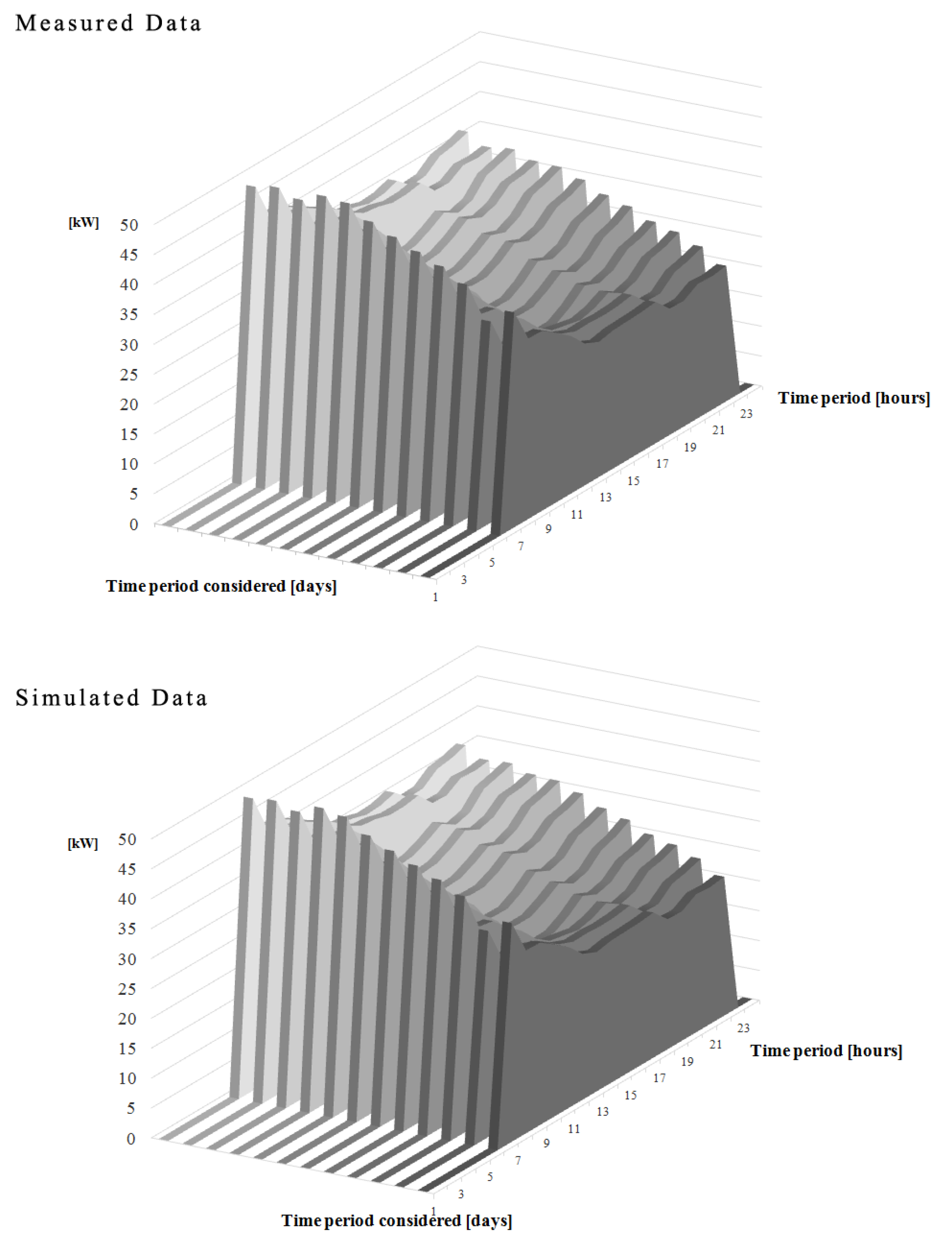
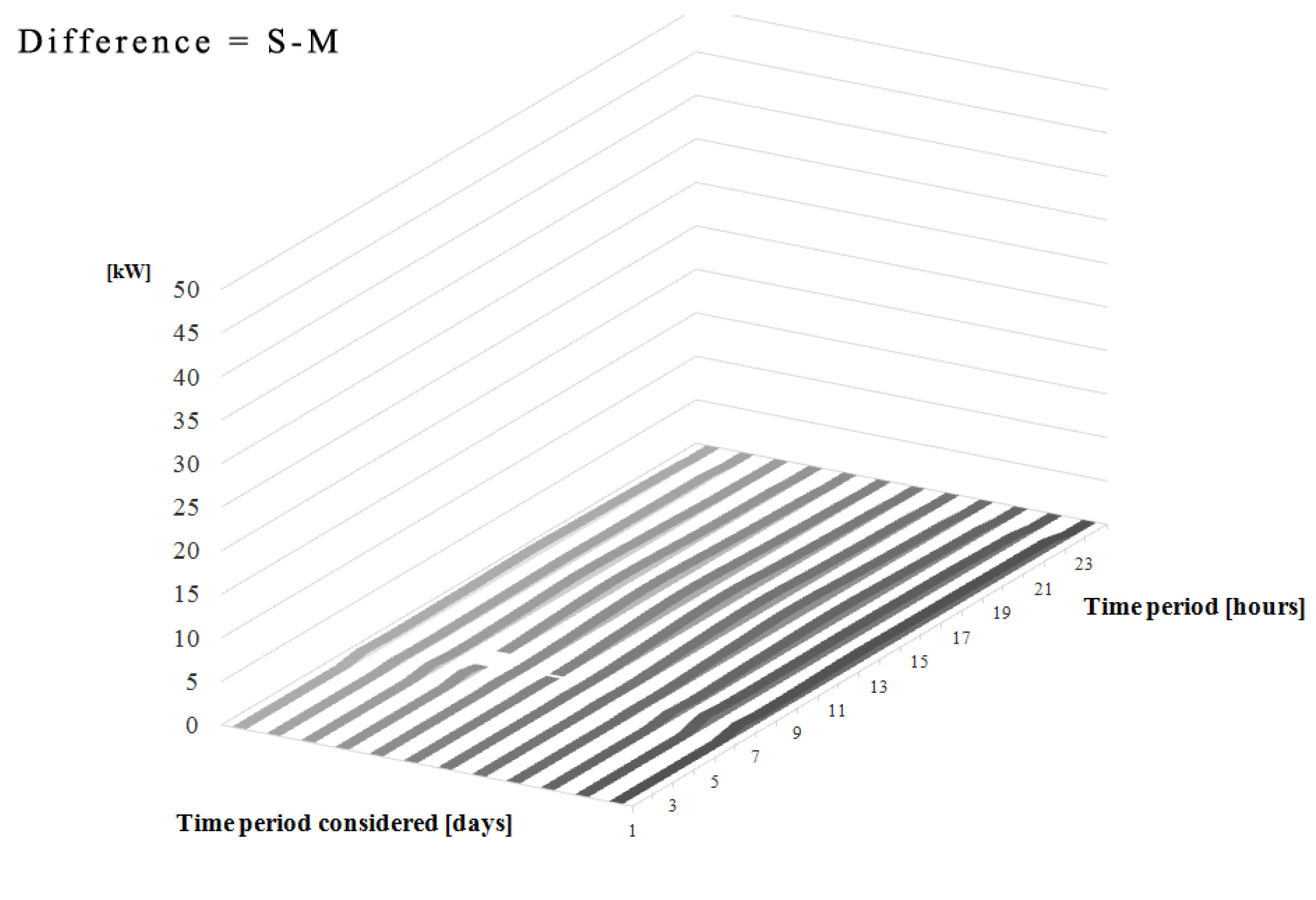
4.2.1. 3D Comparative Plots

A 3D plot approach has been developed to analyze hourly differences, during the whole simulation period, between simulated and measured data [26]. This method is used for calibrating time-dependent parameters, such as schedule loads. Hourly values are computed and compared in the plot. The originality of this method relies on the increased ease of identifying even small differences in the measured and simulation data comparison. An example 3D plot, created by the authors and pictured in Figure 1 shows on a daily basis three different D graphical plots, representing measured data, simulated data and the difference between simulated and measured data, respectively. This type of representation has also been used with statistical indices (MBE and Cv(RMSE)) for analyzing the goodness-of-fit of the building model.

Figure 1. Example of 3D comparative plots.

Figure 1. Example of 3D comparative plots.

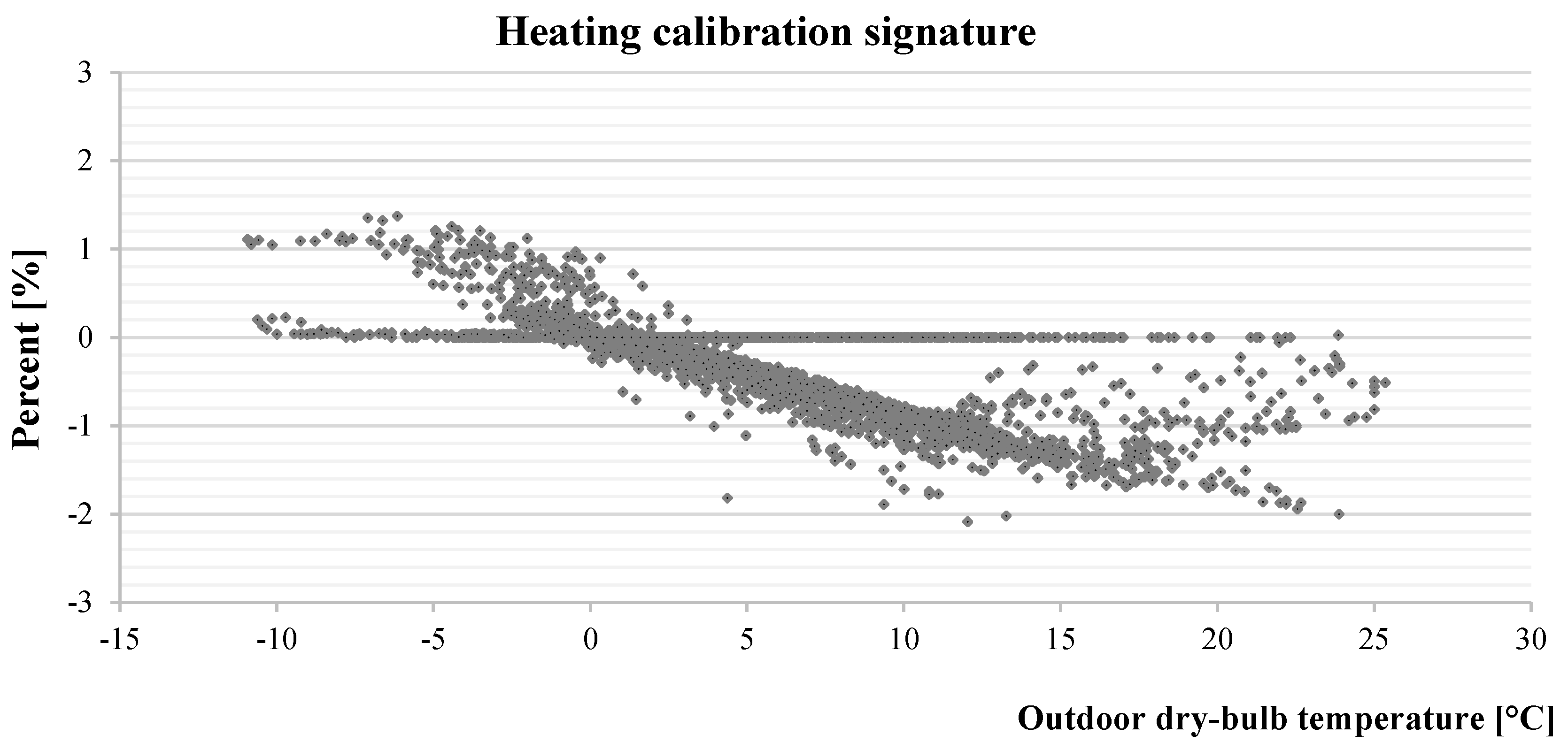
4.2.2. Calibration Signature

The term signature is used to refer to a graphical representation of the difference between the simulated and the measured energy performance of a particular case study [27]. It corresponds to a normalized plot of the differences between the predicted and simulated energy consumption, as a function of the outdoor air temperature.

$$Residual=S-M$$

(5)

$$Calibration signature = \frac{- Residual }{M_{maximum}}\times 100\%$$

(6)

For each temperature, the difference between measured and simulated energy values, divided by the maximum measured energy value and multiplied by 100%, is plotted versus the temperature, to draw the trend of the signature. For a model perfectly calibrated the signature should be a flat line. An example calibration signature is depicted in Figure 2.

Figure 2. Example of calibration signature.

Figure 2. Example of calibration signature.

Another signature, referred as characteristic signature, should be defined for comparing values from two distinguished simulations, instead of values from measured and simulated data. The characteristic signature should be taken as reference or baseline for the measured values. Characteristic signatures are generally calculated based on a daily average basis and are denoted by a characteristic shape due to the climate and the system type considered.

$$Characteristic signature= \frac{Change in energy consumption}{M_{maximum}}\times 100\%$$

(7)

When assessing both characteristic and calibration signatures, the differences between the two curves help users detect errors in the simulation inputs for calibrating the model. It is thus possible to study the effect of the input parameters variation in the building models looking at the calculated signature.

A proposed methodology based on the use of the calibration and characteristic signatures is presented in [27] as a fast procedure. Assessed for both heating and cooling consumption, usually the calibration signature is compared to the characteristic signature of the investigated system configuration or studied climate, to verify if, varying one or more parameters, the signatures are similar, and an acceptable value of the combined error, ERROR_TOT, is reached. This error is calculated as follows:

$$ERRO{R}_{TOT}= \left[\left(RMS{E}_{CLG}^2+RMS{E}_{HTG}^2\right)+\left(MB{E}_{CLG}^2+MB{E}_{HTG}^2\right)\right]$$

(8)

where

• subscripts _HTG and _CLG refer, respectively, to the heating and cooling time intervals considered;
• RSME is the Root Mean Squared Error calculated as in Equation (3); and
• MBE is the Mean Bias Error calculated as in compliance with Equation (1).

When the minimum of ERROR_TOT is achieved, then the calibration can be considered concluded.

Several applications of this methodology can be found in research and academic US studies [28,29,30]. In particular, it has been presented within Sub-Task D2 of the International Energy Agency ECBCS Annex 40 “Commissioning of Buildings and HVAC Systems for Improved Energy Performance” [31].

4.3. Calibration Based on Analytical Procedures

This category is based on analytical and test procedures, such as short or long-term monitoring periods. It can be distinguished from the automated methodologies as it does not employ mathematical or statistical procedure for the calibration process.

Among the special tests that can be used for calibrating the building models, measurement tests (such as blower door tests or wall thermal transmittance measures) are considered. As they are quite invasive, especially when buildings are constantly occupied, they cannot always be performed.

Short-term monitoring and in situ inspections can also assist the calibration process. For example, the PSTAR (Primary and Secondary Term Analysis and Renormalization) method [32] is a unified method of hourly simulations of a building and analysis of performance data, based on the use of short-term monitoring data.

The building energy balance is assessed as sum of the heat flows calculated after the audit inspection. Heat flows are assessed based on macro-dynamic calculations. Each heat flow term is then classified as primary or secondary depending on its magnitude. Primary terms are then renormalized (calibrated) based on monitored data.

Within this category, calibrations that are assisted by audit reports are also included. This builds on building verification from the audit information and technical specifications.

4.4. Automated Techniques for Calibration Based on Analytical and Mathematical Approaches

Automated techniques include all approaches that cannot be considered user driven and are built on sort of automated procedures [19]. They can be based on mathematical procedures (e.g., Bayesian calibration) or analytical approaches.

4.4.1. Bayesian Calibration

Bayesian analysis is a statistical method that employs probability theory to compute a posterior distribution for unknown parameters (θ) given the observed data (y). It is used for calibration purposes for incorporating directly uncertainties in the process [33,34]. Traditionally, the Bayesian technique was used for the model predictions in other domains (such as geochemistry [35] or geology [36,37]) rather than in building physics simulation. However, recently different studies [38,39,40] have focused on the application of this technique to the building simulation domain.

Based on the Bayesian theory [41], a set of values of the uncertain parameters θ of the energy model is formulated in order to find a matching between the simulation outcomes and the measured data y. Three different sources of uncertainty are investigated: parameter uncertainty in the energy model; discrepancy δ(x) between the energy model and the real building behavior; observation error ε(x). A prior probability density function is assigned to each calibration uncertain parameter based on users’ judgment and experience.

The formulation adopted for denoting the observation y(x) is the following:

$$y\left(x\right)= \text{η}\left(x,\text{θ}\right)+\text{δ}\left(x\right)+\text{ε}\left(x\right)$$

(9)

Observations (y) are calculated as a results of simulation outcomes from the model (η(x, θ)) having known parameters (x), unknown parameters (θ), observation errors (ɛ(x)) and discrepancies δ(x). A Gaussian process, based on a multivariate normal vector is adopted to denote η(x,θ) and δ(x). The energy model outputs are thus denoted as normal distribution. In order to solve the multivariate distribution the Markov Chain Monte Carlo algorithm is used to compute the probability density function of the calibration parameters considered. Finally a posterior distributions function of each uncertain parameter is assessed.

4.4.2. Meta-Modeling

According to Van Gelder et al. [42], a meta-model is a mathematical function which coefficients are determined based on a limited number of input/output combinations. Different meta-models techniques can be found in literature [42]: polynomial regression (PR), multivariate adaptive regression splines (MARS), kriging (KR), radial basis function networks (RBF), and sigmoidal neural networks (NN).

A meta-model can be defined as a “model of a model” [43] or a surrogate model that is usually used for reducing the model complexity. It is thus a simpler and computationally faster version of the model. For instance, meta-models created within building simulation programs are based on an essential characterization of the building. This type of building energy models is defined by varying all of the input parameters of the original and more complex model within a certain range, around its baseline design. Usually for creating an n sample of the p inputs, sampling techniques, like in the Monte Carlo Analysis as further described in the paper, are used.

Once the meta-model is derived from the full original model, an optimization algorithm is applied. One of the main benefits of meta-modeling is the reduced simulation time that allow different optimization scenarios to be performed. Meta-modeling is also employed as sensitivity analysis for the assessment of the building energy performance.

4.4.3. Optimization-Based Methods

The term optimization is used in building simulation to refer to an automated approach based on numerical simulation and mathematical optimization [44,45]. Optimization-based methods are usually built on the coupling between a building simulation software (e.g., EnergyPlus, TRNSYS, etc.) and an optimization program (e.g., GenOpt), which employs optimization algorithms [45,46,47]. Simulation-based optimization has recently been used for various applications in building simulation [48,49,50], and also for the calibration of building models [43,51]. In order to perform the optimization, an objective function has to be set within the optimization program. Usually in calibration application the objective function is defined as a function of the difference between measured and simulated data. The optimization is thus based on the matching between a set of measured data and simulated data.

5. Model Uncertainties

Uncertainty and sensitivity analyses represent an integral part of the modeling process, especially for calibrated simulation. Saltelli et al. [52] claimed the relevance of sensitivity analyses in the modeling process models when dealing with uncertainties, treating the choice of the model as one of the sources of uncertainty. Recently uncertainty and sensitivity analyses have found applications in various engineering fields and especially in the building physics domain [18,33,39,53,54,55,56,57,58,59,60,61,62,63,64]. They can help overcoming gaps in the building knowledge, identifying and ranking the sources of uncertainties. As Campolongo et al. [54] stated, “uncertainty and sensitivity analyses study how the uncertainties in the model inputs (X₁, X₂, …, X_k) affect the model response Y”. The uncertainty analysis (UA) aims to quantify the output variability. On the other hand, as claimed by Saltelli et al. [41] “sensitivity analysis (SA) is the study of how the uncertainty in the output of a model can be apportioned to different sources of uncertainty in the model input”.

Notwithstanding uncertainties are often overlooked in calibration studies and not included in calibration methodologies. They are referred as procedural techniques [19] that can be used to assist improving the calibration process. Nevertheless, considering that calibration is a highly under-determined problem, it is important to account for uncertainties in the model during CS. Uncertainties can thus hold a great potential for the design practice. Their identification can have a great impact on the model reliability. Uncertainty analyses may assist calibration for better probabilistic predictions, especially when analyzing different retrofit scenario or during commissioning. In fact even when the building model is created upon the “best plausible estimates”, in terms of input parameters values and building system and operation definition, disagreements between simulated and measured energy consumption may be encountered. Such discrepancies may be attributed to an incomplete knowledge of the building; the building model may thus not reflect correctly the real behavior of the building intended to be simulated.

In the building physics domain, uncertainties may result from different sources. Heo [34] identified four main categories of uncertainty sources in building models, when carrying out studies on energy retrofit analyses. Table 3 lists them.

Table 3. Source of uncertainty in building energy models [34].

Category	Factors
Scenario uncertainty	Outdoor weather conditions
	Building usage/occupancy schedule
Building physical/operational uncertainty	Building envelope properties
	Internal gains
	HVAC systems
	Operation and control settings
Model inadequacy	Modeling assumptions
	Simplification in the model algorithm
	Ignored phenomena in the algorithm
Observation error	Metered data accuracy

Table 3. Source of uncertainty in building energy models [34].

Category	Factors
Scenario uncertainty	Outdoor weather conditions
	Building usage/occupancy schedule
Building physical/operational uncertainty	Building envelope properties
	Internal gains
	HVAC systems
	Operation and control settings
Model inadequacy	Modeling assumptions
	Simplification in the model algorithm
	Ignored phenomena in the algorithm
Observation error	Metered data accuracy

All four categories refer to uncertainties in the physical domain of the building. The first category “Scenario uncertainty” concerns the external environment (e.g., outdoor weather conditions) and the building use. Usually, real weather data are used for creating real weather file to be employed in simulation instead of TMY weather data. Incomplete and fragmented data can determine uncertainties in the data collection and consequently in the definition of the real weather data. Similarly, uncertainties can affect the definition of the building use, which is set by means of schedules expressing the building occupancy and operation. The second category refers to uncertainties in the building modeling, with special regard to the building envelope thermo-physical properties, the building internal gains (people, appliances, lightings, etc.), the HVAC definition and its operational and control settings. The third category refers to uncertainties in the building model as physical representation of the real phenomena. Each building model is thus an approximation of a real building, created on the basis of assumptions and simplifications. The last category refers to observation errors in the measured data. The data quality of measurement used for calibrating the model can affect the accuracy of the results. Therefore uncertainties in measured data have thus to be taken into account.

From literature, different methods for SA and UA can be applied. First, it is essential to distinguish two main approaches: external and internal methods [55]. Within internal methods fall all those approaches where, the mathematics equations, which the simulation models are built on, are not subjected to review. Internal methods won’t be described within the present paper, as the focus of this section will be on uncertainties coming from outside the system. The deterministic approach used for defining and simulating the building models is not discussed. Indeed, external methods include all methods aiming to alter the simulation model parameters and measure the effect of their variation on the outputs. Under the umbrella of the external methods two different categories can be identified [54]: local and global approaches. The first category includes both screening methods and local methods. They are both considered One At a Time (OAT) method as one parameter (input data) is varied at time while all the others are maintained constant. Uncertainties in one parameter are thus calculated for studying how the variations affect the model output. Interactions between different model inputs are therefore overlooked. Global sensitivity methods are, on the other hands, based on varying more parameters simultaneously. They study thus the influence of uncertain input on the whole space.

5.1. Screening-Based Method

Screening analyses are local sensitivity analyses usually aimed at identifying the most important or influent parameters to be considered in further global SA.

5.1.1. Sensitivity Index

It is an OAT method and one of the simplest methods for screening the most important parameters over the investigated output in a model. Standard values and two extreme values on the standard one (minimum and maximum values) are defined for the studied model parameters. To evaluate the sensitivity of each parameter a specific measure, the sensitivity index (SI) is calculated. It corresponds to the output difference, in %, for the extreme values of the parameter considered. It is calculated for each parameter once at time. It is formulated as follows [57]:

$$SI= \frac{E_{max}- E_{min}}{E_{max}}\times 100\%$$

(10)

When the parameter SI changes considerably, the parameter can be considered sensitive, thus influent.

5.1.2. Differential Sensitivity Analysis

Another simple method used for carrying out a sensitivity analysis is the Differential Sensitivity Analysis method (DSA) [64]. Each parameter is varied once at a time. The measure used for assessing the variation of the input on the studied output is the influence coefficient (IC). It is a non-dimensional measure calculated as follows:

$$IC=\frac{\frac{\mathrm{\Delta }OP}{O{P}_{bc}}}{\frac{\mathrm{\Delta }IP}{I{P}_{bc}}}$$

(11)

where

• OP is the output data value;
• IP is the input data value; and
• the subscript _bc indicates the values referring to the baseline model.

Usually DSA is employed in compliance with other screening techniques, like the Morris method [18,64].

5.1.3. Elementary Effects

The most common screening technique is the Morris method, also known as method of the “Elementary Effects” (EE) [54,65]. It is an OAT method as well. It is one of the most effective local SA methods due to its global approach. For this reason it also considered a global SA method rather than a local one. The model sensitivity to the parameter analyzed is investigated through two measures: the mean value and standard deviation of the computed EE for each factor investigated. They are both used to rank the parameters for their influence on the output considered. For this reason this method is also referred as the EE method. The EE of a given parameter X_i at a given point is formulated as follows [54,56]:

$$E{E}_i= \frac{Y\left(x_1,x_{i-1},x_i+{\mathrm{\Delta }}_{i+1},\dots ,x_k\right)-Y\left(x_1,\dots ,x_k\right)}{{\mathrm{\Delta }}_i}$$

(12)

where

• Y is the system output evaluated before and after the variation of the i_th parameter; and
• Δ is an incremental effect that is a multiple of 1/(p − 1).

As different trajectories are defined each time a new parameter is changed, the baseline value is every time different.

For each factor k, r different elementary effects, as r different trajectories, are sampled. The mean values μ_i of the sample of r value of EE_i, as measure of the overall effect of the input X_i on the output Y, is then assessed. Moreover, the standard deviation σ_i of each of the k distributions of values of EE_i, as an expression of the interactions effects, is also computed. The formulation for μ_i and σ_i are, respectively, presented in Equations (12) and (13):

$${\text{μ}}_i=\frac{{{\displaystyle \sum }}_{j=1}^{r}E{E}_i(X^j)}{r}$$

(13)

$${\text{σ}}_i=\sqrt{\frac{{{\displaystyle \sum }}_{j=1}^r{[E{E}_i(X^j)-{\text{μ}}_i]}^2}{r}}$$

(14)

The results are usually plotted in the typical two-dimensional graph proposed by Morris [65]. Mean values μ for each parameter (on the X-axe) are compared to the corresponding standard deviation σ (on the Y-axe). The points with the highest values of both the measures are the most critical for calibration. The parameters with high standard deviations but low mean have also to be considered influential for calibration, as the lower values of μ can be attributed to compensation errors (negative and positive values).

A revised version of the Morris method has been developed by Saltelli et al. [18,54,56]. Instead of the mean value calculation, this version is based on the absolute value of the mean, μ_i^∗, in order to avoid cancellation errors.

$${\text{μ}}_i^{*}=\frac{{{\displaystyle \sum }}_{j=1}^r{\left|E{E}_i (X^j)\right|}_i()}{r}$$

(15)

The EE method does not allow UA as it does not take into account the shape of probability density function of the parameters. It cannot be considered a quantitative analysis as it does not quantify the parameters influence. However this method can be used to isolate the very few influent parameters and rank them among a large number of studied parameters. For this reason it has been widely employed in building energy analyses and in the first stages of calibrated simulation [38,64,66,67].

5.2. Regression Analysis

Regression analysis are used both in the early design stages, for considering different design scenarios and their impact on the building energy consumption, and in post-construction stages, for assisting the calibration of building models. Regression equations are thus employed for carrying out global sensitivity analysis to identify the most influencing parameters in the energy consumptions of the building model to be calibrated [41]. It is a method commonly used to reduce the computational costs. As statistical method, it aims to estimate the relationships between different variables in a model, investigating how a dependent variable changes based on the variation of an independent variable. Specifically it aims to estimate the regression function, which is the function of the independent variable. In particular standardized regression coefficients are used in SA for applying sensitivity rankings to the input parameters [41]. They represent a mean of the parameter influence on the model. Based on the relative magnitude of the regression coefficients, a sensitivity ranking is assessed.

Applications of similar mathematical models to the domain of building simulation can be found in literature [62,63,68,69].

5.3. Variance-Based Method

Variance-based methods aim to decompose the uncertainty of the outputs over the input variables. Usually two main sensitivity measures are assessed within this type of technique:

-

first-order index, S_i, which represents the effect of the input parameter X_i on output variation y;

-

total order index, S_Ti, that measures the effect of the parameter alone and the sensitivity of the interaction of the parameter with all other parameters, as described in Equation (16).

S_Ti = S_i + S_ij + S_ik + … + S_ijk + …

(16)

The variance-based method can cope with non-linear and non-monotonic models and appreciate the interaction effects among input factors.

5.3.1. ANOVA

The Analysis Of Variance (ANOVA) technique is a variance-based method used for global sensitivity analysis purpose [70,71]. This is a statistical technique where the output variance is divided over the input variables. The variance is a measure of the output dispersion, used to assess the relevance of each input design variable. This technique is based on the decomposition of the model variance into first-order index, second-order or higher-order indices and the total effect index.

5.3.2. FAST

The Fourier amplitude sensitivity test (FAST) was first introduced by Cukier et al. [72] in the 1970s and used for carrying out global SA of mathematical models. The classical FAST method [72] was used to compute only the first order sensitivity index S_i, while an extended version has been later proposed by Saltelli et al. [73] for the simultaneous estimation of the first and total sensitivity index, respectively, S_i and S_Ti, for a given factor X_i [41].

The FAST method is considered superior to other local SA methods as it allows apportioning the output variance to the variance in the input parameters [73]. It computes the individual contribution of each input factor, referred as “main effect” in Statistics, to the output variance [41,73].

Sobol [41,73] has developed a global SA method, which is considered a natural and more general extension of the FAST approach. In this case, the main effect, S_i, and the interaction terms, S_ij, are calculated together with higher-order terms computed by means of MCA. Both FAST and Sobol’s method allow the evaluation of each parameter contribution to the variance caused by the main effect, however FAST is computationally faster than Sobol’s that decomposes all the output variance indeed.

5.4. Monte Carlo Method

Monte Carlo analysis (MCA) is one of the most commonly used techniques for carrying out global sensitivity and uncertainty analysis [43,59,67,74,75,76,77,78]. It is based on a repeated number of simulations with a random sampling of the models input. Each uncertain model input is defined through a probability distribution. All input parameters are then varied simultaneously. MCA assesses an estimate of the overall uncertainty in the model predictions based on the uncertainties in the input parameters.

Different techniques may be used for sampling the data: random, stratified sampling and Latin Hypercube Sampling [79]. In the first case the input values are a random sample from the probability distribution. Stratified sampling is an improvement of the random technique that, based on the subdivision of the probability distribution of the input factor into different strata of equal probability, force the sample to conform to the whole distribution studied [80]. Latin Hypercube sampling is a stratified sampling where the values generated for each input factor come from a different stratum.

MCA is based on a matrix that contains, for N model runs, the randomly generated sample values of each of the input parameters under examination. MCA allows a better coverage of the sample space of the input parameters [77] as, for example with a Latin Hypercube Sampling, N, then evaluated N times, once for each row of the sample, creating an input-output map within the parameters.

6. Calibrated Simulation Applications

A list of the main and most recent applications of CS is reported in Table 4. All studies are classified according to some criteria characterizing the calibration process:

-

the calibration methodology adopted;

-

the calibration level pursued;

-

the model complexity;

-

the simulation tool used; and

-

the integration of SA/UA in the calibration process.

Reddy et al. [6] presented a four-step general methodology for calibrating building models, which is accompanied by a detailed review of calibration techniques [17] and applied to three case studies [16]. The methodology proposed does not aim to find a unique and best calibrated solution but it rather aims to find a small set of most plausible solutions indeed. Although tested with the DOE-2, in the ASHRAE research project 1051-RP, the methodology can be applied to any simulation program. It was developed as a robust but flexible methodology for calibrating building models. The core of the methodology is represented by the sensitivity analysis for identifying the parameters that influence the most the model outputs during calibration. First a set of influential parameters are defined with their best-guess value; secondly Monte Carlo simulations are run to filter and to identify the more sensitive parameters to be tuned for calibration. The case studies were investigated for the calibration level 4. After sensitivity analysis is performed, a set of the most plausible solutions for the parameters tuning is defined to make the measured consumption match the predicted ones from the simulation program. The methodology has also been applied to other case studies [81] and used for research activities [82].

Bertagnolio et al. [18] developed an evidence-based calibration methodology intended to be manual but systematic [83] and applied it to a real office building. The application of the developed methodology is quite detailed, and ranges from the calibration level 1 to level 4 (see Table 1 for further specifications). The methodology builds mainly on an intensive use of a sensitivity analysis (Morris method) and (non-intrusive) measurements. The case study was modeled, based on the available measured energy use data, as a simplified building energy model. The accuracy of the building model was verified for each calibration level fulfilling the MBE and Cv(RMSE) statistical indices.

Eisenhower et al. [13] developed a systematic and automated approach for calibrating building energy models. The methodology identifies critical and influential parameters and automatically tunes them to calibrate the building model. In particular, after a first sampling of all the model parameters (2063), a sensitivity analysis was run for ranking the parameters, in terms of their impact on the output results. A quasi-Monte Carlo approach was used as SA. From 2063 input data sampled, a set of top 10 parameters was defined for the calibration stage. In order to reduce the calibration computation time a meta-model of the case study was created within the EnergyPlus program.

Heo et al. [34,38] applied a Bayesian calibration of normative energy models for accounting uncertainties during the retrofitting of existing buildings. Calibration was carried out to assess a set of energy retrofit measures to apply to the case study. The normative energy model of the case study was also compared with a detailed transient model created in EnergyPlus. CS is assisted by the Morris method, to screen and reduce the number of parameters to calibrate. From the results, it emerged that the calibrated normative model predicts as accurately as the calibrated transient model, but requires much lower computation time.

Raftery et al. [84] presented an evidence-based method for CS and applied it to a real monitored building [85]. The method aims to improve the reliability of calibrated models classifying the changes made to the building model depending on a hierarchy of sources. This hierarchy impacts on the source reliability that brings to changes in the model. These changes are stored by a control program that allows the users to review the building model and the changes made to its. After the modeling is completed, an iterative calibration is carried out until the model can be considered calibrated and its accuracy verified.

Taheri et al. [51] carried out an optimization-aided model calibration method and applied it to an existing university building for a five-month calibration period. Based on first monitored data, occupancy schedules were created and implemented in the EnergyPlus building model. An objective function, based on the difference between the measured and simulated zone mean air temperature was defined to calibrate the building model. The calibration process was divided into four steps in order to investigate and tune the most influent parameters, in the building model; starting from a number of eight parameters in the first calibration, the number of parameters investigated was reduced to two in the second and third calibrations, and to one in the fourth and fifth calibrations. The same method was also applied to other case studies [86,87,88].

Maile et al. [20] developed a method, named Energy Performance Comparison Methodology (EPCM), for providing feedback in the building design and operation, and especially for investigating the buildings performance problems based on a comparison of measured and simulated energy performance data. The EPCM is a three-step method: preparation, matching, and evaluation steps.

Another interesting two-step methodology was proposed by Palomo del Barrio et al. [89], with specific regard to the validation of empirical models. Based on the analysis of the model parameters space, the methodology first checks the model validity to detect significant disagreements between measurements and simulations in the model performance (sensitivity analysis), and then investigates the differences between model simulations and measurements (optimization of model parameters).

7. Conclusions

Due to recent interest both in studies concerning the disagreement between measured building energy consumption and predicted energy consumption by building energy simulation programs and in the assessment of the occupant behavior, the application of calibration has expanded. Assessment of occupant behavior also involves sensitivity and uncertainty analyses, since the occupancy related to the building usage is one of the main sources of uncertainty in the building simulation models. However, despite the increasing importance and use of CS, the lack of a harmonized and officially recognized procedure for performing calibration of building energy models still remains a major issue.

This study reviews the most used calibration methodologies in the domain of building simulation, aiming to highlight the pros and cons of the calibration and pointing out criticalities and gaps of such methodologies. With regard to the model complexity, automated models, based on mathematical and statistical techniques, tend to use simplified models, rather than more detailed ones, in order to reduce computational time. Manual and graphical methods may also avoid the use of highly complex models. Complex models are in fact hard to handle and to tune when using both manual methods and automated procedures. Additionally, automated methods may bring a reduction on the computational time of the calibration process. Of course even if automated methods can provide guidance to “non-properly” experienced users towards calibration, they may represent procedures, which are too complex, bringing users to a confusing and unorganized process. User’s skills and knowledge constitute an essential and primary element for performing calibration; they thus directly impact on the calibration running time, regardless of the calibration method applied and the accuracy of the building models achieved.

Among the methods presented some are emerging more than others, being applied in many studies. The current trend, based on the literature review hereby presented, is the search for and use of automated methods, based on the implementation of sensitivity and uncertainty analysis, to fine-tune the models and improve thus their accuracy. This is particularly true for complex dynamic models of buildings that are used by professionals. In many cases, it is possible to have large sets of measured data, however, due to the high number of parameters of a dynamic model and the computational time necessary, the process of calibrating the model is done merely with a trial error approach. Application in the design professionals’ community is the challenge that calibrated simulation will face in the next future.

Table 4. List of the most recent published application CS in the domain of building simulation.

Author	Title	Year	Journal/Conference	Ref.	Calibration Characterization
					Model type		Calibration level	Calibration Method		SA/UA	Monitoring period	Simulation tool or Standard
Palomo del Barrio, E.; Guyon, G.	Application of parameters space analysis tools for empirical model validation	2004	Energy and Buildings, 36, 23-33	[89]	-	whole building model	-	-	Optmi-zation	SA	-	CLIM2000
Liu, S.; Henze, G.P.	Calibration of building models for supervisory control of commercial building	2005	9th International Building Simulation Association (IBPSA) Conference 2005	[48]	Detailed	whole building model	-	Automated	Optmi-zation	-	-	EnergyPlus, GenOpt
Pan, Y.; Huang, Z.; Wu, G.	Calibrated building energy simulation and its application in a high-rise commercial building in Shanghai	2007	Energy and Buildings, 39, 651-657	[12]	Detailed	whole building model	Level 3	Manual	Iterative	-	-	DOE-2
Reddy, T.A.; Maor, I.; Panjapornpon, C.	Calibrating Detailed Building Energy Simulation Programs with Measured Data–Part II: Application to Three Case Study Office Buildings (RP-1051)	2007	HVAC and Research, 13, 221-241	[16]	Detailed	whole building model	Level 4	Mathema-tical	-	Montecarlo	N.A.	DOE-2
Hassan, M.A.; Shebl, S.S.; Ibrahim, E.A.; Aglan, H.A.	Modeling and validation of the thermal performance of an affordable, energy efficient, healthy dwelling unit	2011	Journal of Building Simulation 4, 255-262	[24]	Detailed	whole building model	Level 4-5	Manual	Iterative	-	Short-term	Visual DOE-4
Liu, G.; Liu, M.	A rapid calibration procedure and case study for simplified simulation models of commonly used HVAC systems	2011	Building and Environment 46, 409-420	[28]	-	whole building model	Level 4	Graphical	Calibration Signature	NA	Short-term	-
Raftery, P.; Keane, M.; Costa, A.	Calibrating whole building energy models: Detailed case study using hourly measured data	2011	Energy and Buildings 2011, 43, 3666-3679	[85]	Detailed	whole building model	Level 4	Manual	Iterative	-	Long-term	EnergyPlus
Bertagnolio, S.; Randaxhe, F.; Lemort, V.	Evidence-based calibration of a building energy simulation model: Application to an office building in Belgium	2012	12th International Conference for Enhanced Building Operations, Manchester, UK	[83]	Normative (quasi-steady)	whole building model	Level 1 to 4	-	evidence-based	Morris Method	Short-term	ISO 13790
Heo, Y.; Choudhary, R.; Augenbroe, G.A.	Calibration of building energy models for retrofit analysis under uncertainty	2012	Energy and Buildings 47, 550-560	[38]	Normative (quasi-steady)	whole building model	-	Mathema-tical	Bayesian	Morris Method	-	ISO 13790
Fontanella,G.; Basciotti, D.; Dubisch, F.; Judex, F.; Preisler, A.; Hettfleisch, C.; Vukovic, V.; Selke, T.	Calibration and validation of a solar thermal system model in Modelica	2012	Journal of Building Simulation 5, 293-300	[25]	Detailed	Solar System	Level 4	-	Optmiza-tion	-	Short-term	Modelica (Dymola), GenOpt
Maile, T.; Bazjanac, T.; Fischer, M.	A method to compare simulated and measured data to assess building energy performance	2012	Building and Environment 56, 241-251	[90]	Detailed	whole building model	N.A.	Manual	Iterative	-	Long-term	Not specified
Parker, J.; Cropper, P.; Shao, L.	A calibrated whole building simulation approach to assessing retrofit options for Birmingham airport	2012	IBPSA-England, 1st Building Simulation and Optimization Conference, Loughborough, UK	[91]	Detailed	whole building model	Level 2	Manual (Raftery et al.)	Iterative	-	Long-term	IES
Kim, Y.; Yoon, S.; Park, C.	Stochastic comparison between simplified energy calculation and dynamic simulation	2013	Energy and Buildings 64, 332-342	[59]	Simplified (A), detailed (B)	whole building model	-	Matema-tical	Bayesian	SA-Morris Method	-	ISO 13790 (A), EnergyPlus (B)
Manfren, M.; Aste, N.; Moshksar, R.	Calibration and uncertainty analysis for computer models–A meta-model based approach for integrated building energy simulation	2013	Applied Energy 103, 627-641	[39]	Simplified and detailed	whole building model	Level 4	Mathema-tical	Bayesian, Meta-modelling	with Bayesian calibration	Short-term	-
O’Neill, Z.; Eisenhower, B.	Leveraging the analysis of parametric uncertainty for building energy model calibration	2013	Journal of Building Simulation 5, 365-377	[13]	meta-model	whole building model	Levels 4-5	Automated	Optmi-zation	quasi-Montecarlo approach	Long-term	EnergyPlus, Design-Builder
Taheri, M.; Tahmasebi, F.; Mahdavi, A.	A case study of optimization-aided thermal building performance simulation calibration	2013	13th Conference of IBPSA Chambéry, France	[51]	Dynamic	whole building model	Level 4	Automated	Optmi-zation	-	Short-term	EnergyPlus, GenOpt
Mihai, A.; Zmeureanu, R.	Calibration of an energy model of a new research center building	2014	13th Conference of IBPSA Chambéry, France	[92]	Dynamic	whole building model	Level 4	Manual	evidence-based	-	Short-term	eQuest
Mustafaraj, G.; Marini, D.; Costa, A.; Keane, M.	Model calibration for building energy efficiency simulation	2014	Applied Energy 130, 72-85	[93]	Dynamic	whole building model	Level 3-4	Manual	Iterative (based on Bertagnolio and Raftery methods)	SA	Short-term	Design-Builder, EnergyPlus
Penna, P.; Gasparella, A.; Cappelletti, F.; Tahmasebi, F.; Mahdavi A.	Optimization-based calibration of a school building based on short-term monitoring data	2014	10th European Conference on Product and Process Modeling	[88]	Detailed	whole building model	Level 3-4	Automated	Optmiza-tion	-	Short-term	TRNSYS, GenOPt

Table 4. List of the most recent published application CS in the domain of building simulation.

Author	Title	Year	Journal/Conference	Ref.	Calibration Characterization
					Model type		Calibration level	Calibration Method		SA/UA	Monitoring period	Simulation tool or Standard
Palomo del Barrio, E.; Guyon, G.	Application of parameters space analysis tools for empirical model validation	2004	Energy and Buildings, 36, 23-33	[89]	-	whole building model	-	-	Optmi-zation	SA	-	CLIM2000
Liu, S.; Henze, G.P.	Calibration of building models for supervisory control of commercial building	2005	9th International Building Simulation Association (IBPSA) Conference 2005	[48]	Detailed	whole building model	-	Automated	Optmi-zation	-	-	EnergyPlus, GenOpt
Pan, Y.; Huang, Z.; Wu, G.	Calibrated building energy simulation and its application in a high-rise commercial building in Shanghai	2007	Energy and Buildings, 39, 651-657	[12]	Detailed	whole building model	Level 3	Manual	Iterative	-	-	DOE-2
Reddy, T.A.; Maor, I.; Panjapornpon, C.	Calibrating Detailed Building Energy Simulation Programs with Measured Data–Part II: Application to Three Case Study Office Buildings (RP-1051)	2007	HVAC and Research, 13, 221-241	[16]	Detailed	whole building model	Level 4	Mathema-tical	-	Montecarlo	N.A.	DOE-2
Hassan, M.A.; Shebl, S.S.; Ibrahim, E.A.; Aglan, H.A.	Modeling and validation of the thermal performance of an affordable, energy efficient, healthy dwelling unit	2011	Journal of Building Simulation 4, 255-262	[24]	Detailed	whole building model	Level 4-5	Manual	Iterative	-	Short-term	Visual DOE-4
Liu, G.; Liu, M.	A rapid calibration procedure and case study for simplified simulation models of commonly used HVAC systems	2011	Building and Environment 46, 409-420	[28]	-	whole building model	Level 4	Graphical	Calibration Signature	NA	Short-term	-
Raftery, P.; Keane, M.; Costa, A.	Calibrating whole building energy models: Detailed case study using hourly measured data	2011	Energy and Buildings 2011, 43, 3666-3679	[85]	Detailed	whole building model	Level 4	Manual	Iterative	-	Long-term	EnergyPlus
Bertagnolio, S.; Randaxhe, F.; Lemort, V.	Evidence-based calibration of a building energy simulation model: Application to an office building in Belgium	2012	12th International Conference for Enhanced Building Operations, Manchester, UK	[83]	Normative (quasi-steady)	whole building model	Level 1 to 4	-	evidence-based	Morris Method	Short-term	ISO 13790
Heo, Y.; Choudhary, R.; Augenbroe, G.A.	Calibration of building energy models for retrofit analysis under uncertainty	2012	Energy and Buildings 47, 550-560	[38]	Normative (quasi-steady)	whole building model	-	Mathema-tical	Bayesian	Morris Method	-	ISO 13790
Fontanella,G.; Basciotti, D.; Dubisch, F.; Judex, F.; Preisler, A.; Hettfleisch, C.; Vukovic, V.; Selke, T.	Calibration and validation of a solar thermal system model in Modelica	2012	Journal of Building Simulation 5, 293-300	[25]	Detailed	Solar System	Level 4	-	Optmiza-tion	-	Short-term	Modelica (Dymola), GenOpt
Maile, T.; Bazjanac, T.; Fischer, M.	A method to compare simulated and measured data to assess building energy performance	2012	Building and Environment 56, 241-251	[90]	Detailed	whole building model	N.A.	Manual	Iterative	-	Long-term	Not specified
Parker, J.; Cropper, P.; Shao, L.	A calibrated whole building simulation approach to assessing retrofit options for Birmingham airport	2012	IBPSA-England, 1st Building Simulation and Optimization Conference, Loughborough, UK	[91]	Detailed	whole building model	Level 2	Manual (Raftery et al.)	Iterative	-	Long-term	IES
Kim, Y.; Yoon, S.; Park, C.	Stochastic comparison between simplified energy calculation and dynamic simulation	2013	Energy and Buildings 64, 332-342	[59]	Simplified (A), detailed (B)	whole building model	-	Matema-tical	Bayesian	SA-Morris Method	-	ISO 13790 (A), EnergyPlus (B)
Manfren, M.; Aste, N.; Moshksar, R.	Calibration and uncertainty analysis for computer models–A meta-model based approach for integrated building energy simulation	2013	Applied Energy 103, 627-641	[39]	Simplified and detailed	whole building model	Level 4	Mathema-tical	Bayesian, Meta-modelling	with Bayesian calibration	Short-term	-
O’Neill, Z.; Eisenhower, B.	Leveraging the analysis of parametric uncertainty for building energy model calibration	2013	Journal of Building Simulation 5, 365-377	[13]	meta-model	whole building model	Levels 4-5	Automated	Optmi-zation	quasi-Montecarlo approach	Long-term	EnergyPlus, Design-Builder
Taheri, M.; Tahmasebi, F.; Mahdavi, A.	A case study of optimization-aided thermal building performance simulation calibration	2013	13th Conference of IBPSA Chambéry, France	[51]	Dynamic	whole building model	Level 4	Automated	Optmi-zation	-	Short-term	EnergyPlus, GenOpt
Mihai, A.; Zmeureanu, R.	Calibration of an energy model of a new research center building	2014	13th Conference of IBPSA Chambéry, France	[92]	Dynamic	whole building model	Level 4	Manual	evidence-based	-	Short-term	eQuest
Mustafaraj, G.; Marini, D.; Costa, A.; Keane, M.	Model calibration for building energy efficiency simulation	2014	Applied Energy 130, 72-85	[93]	Dynamic	whole building model	Level 3-4	Manual	Iterative (based on Bertagnolio and Raftery methods)	SA	Short-term	Design-Builder, EnergyPlus
Penna, P.; Gasparella, A.; Cappelletti, F.; Tahmasebi, F.; Mahdavi A.	Optimization-based calibration of a school building based on short-term monitoring data	2014	10th European Conference on Product and Process Modeling	[88]	Detailed	whole building model	Level 3-4	Automated	Optmiza-tion	-	Short-term	TRNSYS, GenOPt

References

1. Clarke, J.A. Energy Simulation in Building Design, 2nd ed.; Butterworth Heinemann: Oxford, UK, 2001. [Google Scholar]
2. Hensen, J.L.M.; Lamberts, R. Introduction to building performance simulation. In Building Performance Simulation for Design and Operation, 1st ed.; Hensen, J.L.M., Lamberts, R., Eds.; Spon Press: Oxfordshire, UK, 2011. [Google Scholar]
3. Claridge, D.E. Building simulation for practical operational optmization. In Building Performance Simulation for Design and Operation, 1st ed.; Hensen, J.L.M., Lamberts, R., Eds.; Spon Press: Oxfordshire, UK, 2011. [Google Scholar]
4. Emily, M.; Ryan, E.M.; Sanquist, T.F. Validation of building energy modeling tools under idealized and realistic conditions. Energy Build. 2012, 47, 375–382. [Google Scholar] [CrossRef]
5. Dall’O’, G.; Sarto, L.; Sanna, N.; Martucci, A. Comparison between predicted and actual energy performance for summer cooling in high-performance residential buildings in the Lombardy region (Italy). Energy Build. 2012, 54, 234–242. [Google Scholar] [CrossRef]