
Wheel Torque Distribution of Four-Wheel-Drive Electric Vehicles Based on Multi-Objective Optimization

Abstract
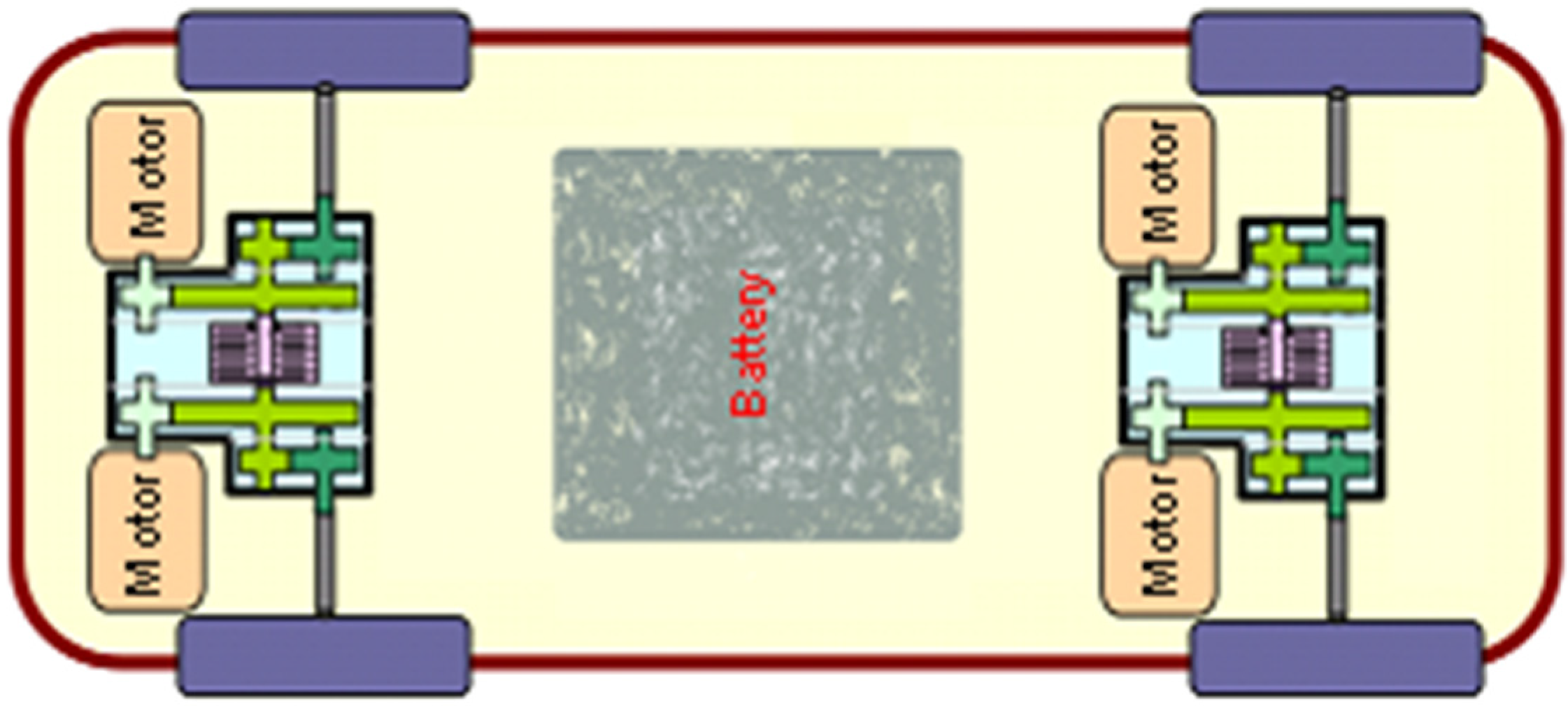
:1. Introduction

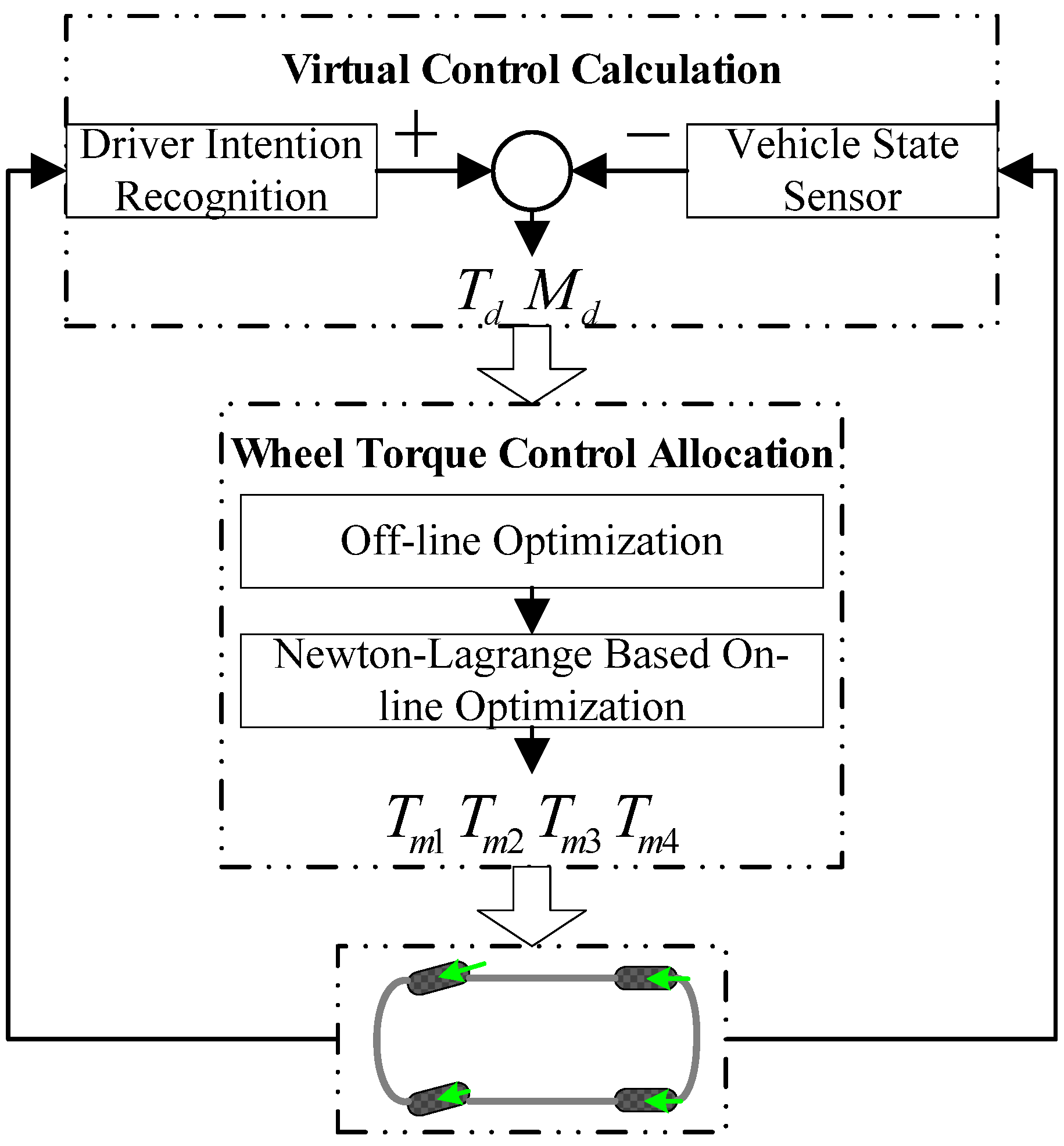
2. The Wheel Torque Control Strategy

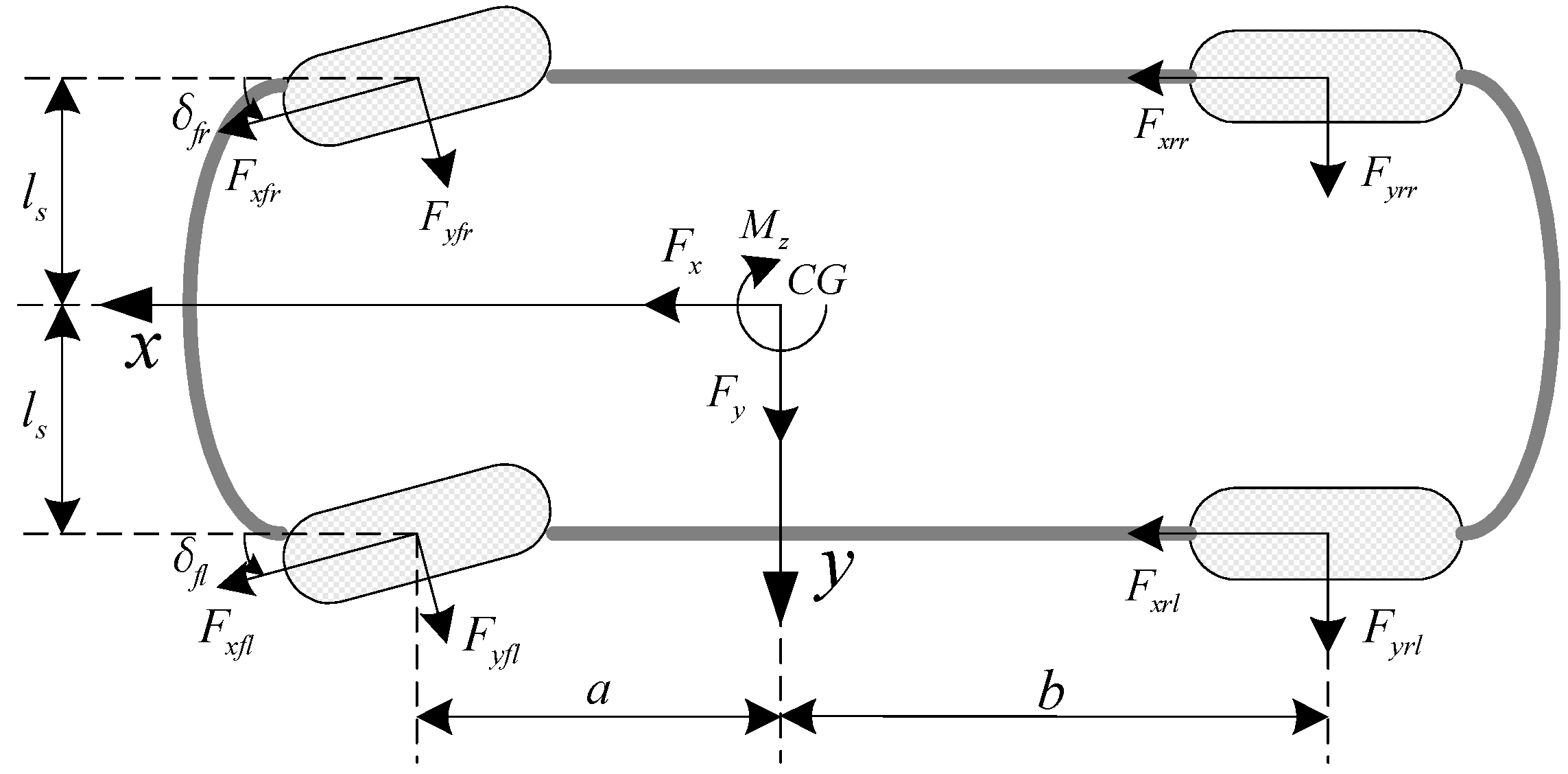
3. Desired Yaw Moment Calculation

4. Wheel Torque Control Allocation
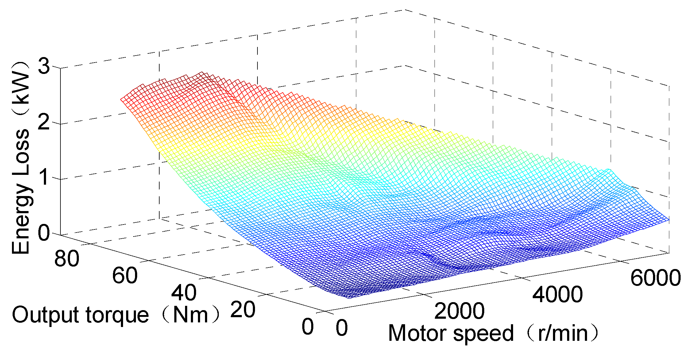
4.1. The Multi-Objective Optimization Algorithm

4.2. Off-Line and On-Line Optimization


5. Simulation and Discussion

| Parameters | Values | Parameters | Values |
|---|---|---|---|
| Vehicle Mass | 1486 kg | Motor Number | 4 |
| Wheelbase | 2.578 m | Motor Rated Power | 8 kW |
| Vehicle Moment of Inertia | 2023 kg·m2 | Motor Peak Torque | 78 Nm |
| Wheel Rolling Radius | 0.298 m | Motor Rated Speed | 2900 rpm |

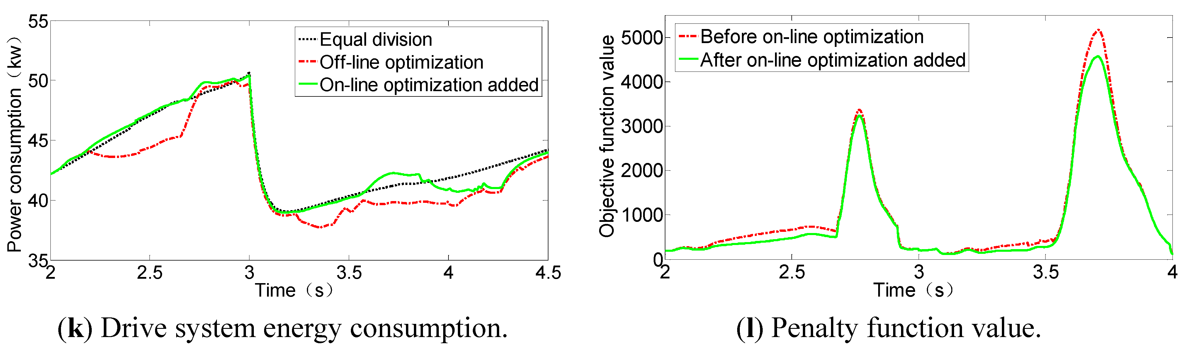
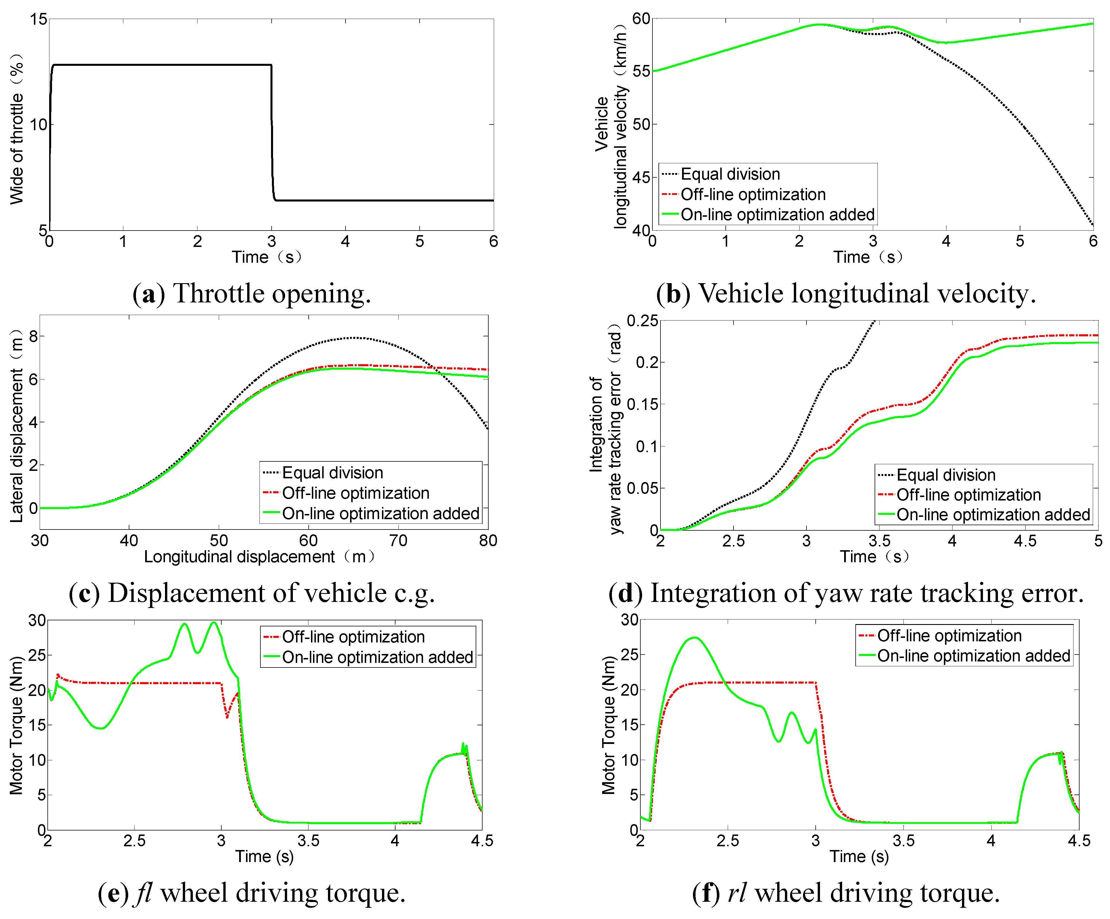
5.1. Large Acceleration Simulation


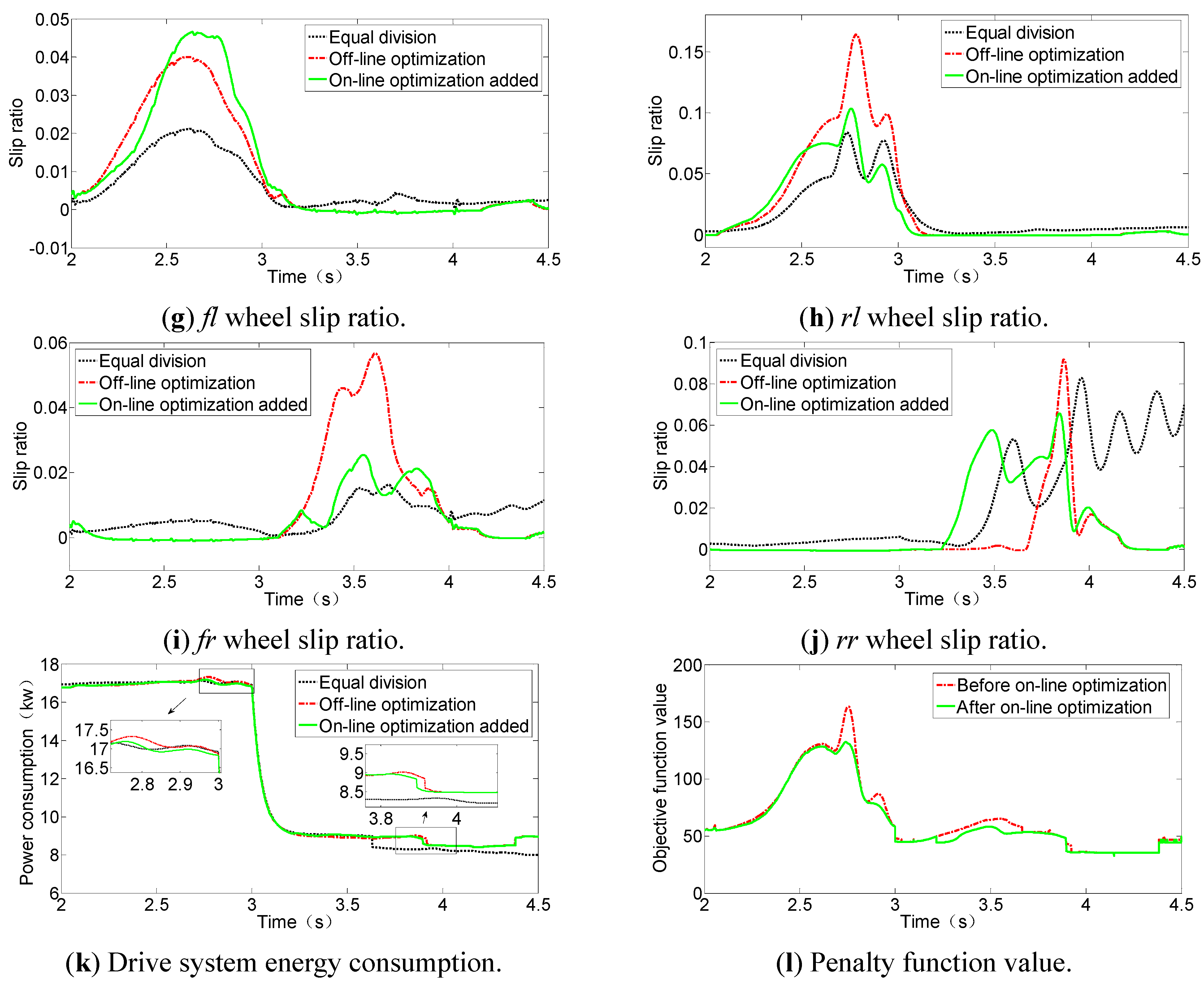
5.2. Small Acceleration Simulation


5.3. Discussion
6. Conclusions
Acknowledgments
Author Contributions
Conflicts of Interest
References
- Wu, T.; Zhang, M.B.; Ou, X.M. Analysis of future vehicle energy demand in China based on a Gompertz function method and computable general equilibrium model. Energies 2014, 7, 7454–7482. [Google Scholar] [CrossRef]
- He, H.W.; Peng, J.K.; Xiong, R.; Fan, H. An acceleration slip regulation strategy for four-wheel drive electric vehicles based on sliding mode control. Energies 2014, 7, 3748–3763. [Google Scholar] [CrossRef]
- Sakai, S.; Sado, H.; Hori, Y. Motion control in an electric vehicle with four independently driven in-wheel motors. IEEE/ASME Trans. Mechatron. 1999, 4, 9–16. [Google Scholar] [CrossRef]
- Lin, C.; Zhang, Z.J.; Ma, J. Dual-motor Anti-slip Differential Drive System. Chinese Patent China 200810097693.5, 2009. [Google Scholar]
- Jeongmin, K.; Chiman, P. Control algorithm for an independent motor-drive vehicle. IEEE Trans. Veh. Technol. 2010, 59, 3213–3222. [Google Scholar] [CrossRef]
- Li, F.Q.; Wang, J.; Liu, Z.D. Motor torque based vehicle stability control for four-wheel-drive electric vehicle. In Proceedings of the IEEE Vehicle Power and Propulsion Conference, Dearborn, MI, USA, 7–11 September 2009; pp. 1596–1601.
- Peng, H.; Hori, Y. Optimum traction force distribution for stability improvement of 4WDEV in critical driving condition. In Proceedings of the 9th IEEE International Workshop on Advanced Motion Control, Istanbul, Turkey, 27–29 March 2006; pp. 596–601.
- He, Z.Y.; Ji, X.W. Nonlinear robust control of integrated vehicle dynamics. Veh. Syst. Dyn. 2012, 50, 247–280. [Google Scholar] [CrossRef]
- Falcone, P.; Tseng, H.E.; Borrelli, F.; Asgari, J.; Hrovat, D. MPC-based yaw and lateral stabilization via active front steering and braking. Veh. Syst. Dyn. 2008, 46, 611–628. [Google Scholar] [CrossRef]
- Javad, A.; Ali, K.S.; Mansour, K. Adaptive vehicle lateral-plane motion control using optimal tire friction forces with saturation limits consideration. IEEE Trans. Veh. Technol. 2009, 58, 4098–4107. [Google Scholar] [CrossRef]
- Wang, R.R.; Chen, Y.; Feng, D.W. Development and performance characterization of an electric ground vehicle with independently actuated in-wheel motors. J. Power Sources 2011, 196, 3962–3971. [Google Scholar] [CrossRef]
- Chen, Y.; Wang, J.M. Energy-efficient control allocation with applications on planar motion control of electric ground vehicles. In Proceeding of the 2011 American Control Conference, San Francisco, CA, USA, 29 June–1 July 2011; pp. 2719–2724.
- Chen, Y.; Wang, J.M. Design and experimental evaluations on energy efficient control allocation methods for over actuated electric vehicles: Longitudinal motion case. IEEE/ASME Trans. Mechatron. 2014, 19, 538–548. [Google Scholar] [CrossRef]
- Leonardo, D.N.; Aldo, S.; Patrick, G. Wheel torque distribution criteria for electric vehicles with torque-vectoring differentials. IEEE Trans. Veh. Technol. 2014, 63, 1593–1602. [Google Scholar] [CrossRef]
- Horiuchi, S.; Okada, K.; Nohtomi, S. Improvement of vehicle handling by nonlinear integrated control of four wheel steering and four wheel torque. JSAE Rev. 1999, 20, 459–464. [Google Scholar] [CrossRef]
- Gu, J.; Ouyang, M.; Lu, D. Energy efficiency optimization of electric vehicle driven by in-wheel motor. Int. J. Automot. Technol. 2013, 14, 763–772. [Google Scholar] [CrossRef]
- Huang, H.X.; Han, J.Y. Mathematical Programming; Tsinghua University Press: Beijing, China, 2006; pp. 289–291. [Google Scholar]
- Lu, P. Constrained tracking control of nonlinear systems. Syst. Control Lett. 1997, 27, 305–314. [Google Scholar] [CrossRef]
- Wang, J.M. Coordinated and Reconfigurable Vehicle Dynamics Control; The University of Texas at Austin: Austin, TX, USA, 2007; pp. 80–104. [Google Scholar]
- Novellis, L.D.; Sorniotti, A.; Gruber, P. Optimal wheel torque distribution for a four-wheel-drive fully electric vehicle. SAE Int. J. Passeng. Cars–Mech. Syst. 2013, 6, 128–136. [Google Scholar] [CrossRef]
© 2015 by the authors; licensee MDPI, Basel, Switzerland. This article is an open access article distributed under the terms and conditions of the Creative Commons Attribution license (http://creativecommons.org/licenses/by/4.0/).
Share and Cite
Lin, C.; Xu, Z. Wheel Torque Distribution of Four-Wheel-Drive Electric Vehicles Based on Multi-Objective Optimization. Energies 2015, 8, 3815-3831. https://doi.org/10.3390/en8053815
Lin C, Xu Z. Wheel Torque Distribution of Four-Wheel-Drive Electric Vehicles Based on Multi-Objective Optimization. Energies. 2015; 8(5):3815-3831. https://doi.org/10.3390/en8053815
Chicago/Turabian StyleLin, Cheng, and Zhifeng Xu. 2015. "Wheel Torque Distribution of Four-Wheel-Drive Electric Vehicles Based on Multi-Objective Optimization" Energies 8, no. 5: 3815-3831. https://doi.org/10.3390/en8053815