System Identification and Resonant Control of Thermoacoustic Engines for Robust Solar Power

Abstract

It was found that thermoacoustic solar-power generators with resonant control are more powerful than passive ones. To continue the work, this paper focuses on the synthesis of robustly resonant controllers that guarantee single-mode resonance not only in steady states, but also in transient states when modelling uncertainties happen and working temperature temporally varies. Here the control synthesis is based on the loop shifting and the frequency-domain identification in advance thereof. Frequency-domain identification is performed to modify the mathematical modelling and to identify the most powerful mode, so that the DSP-based feedback controller can online pitch the engine to the most powerful resonant-frequency robustly and accurately. Moreover, this paper develops two control tools, the higher-order van-der-Pol oscillator and the principle of Dynamical Equilibrium, to assist in system identification and feedback synthesis, respectively.

1. Introduction

Thermoacoustic dynamics can be represented into a feedback-loop interconnected by the heat-transfer dynamics of heating source and the acoustic dynamics of working gas. On the interface with the acoustic subsystem, the heating subsystem in the loop is affected by the temperature fluctuation that is algebraically dependent on the acoustic pressure and the entropy fluctuation thereon. Meanwhile, the heat-flux fluctuation from the heating subsystem initiates acoustic velocity that excites the acoustic motions distributed in the chamber [1,2], and thus forms the feedback loop. Imposed on those mean-flow conditions which characterize large loop-gains, the thermoacoustic dynamics can become linearly unstable up to limit-cycling (nonlinear vibration), or even up to mean-flow buckling (turbulence, streaming, vortex, etc.). Such thermoacoustic instability can be utilized for fast-time propulsion in thermoacoustic engines [3,4,5,6], but should be suppressed in combustion chambers to avert a variety of combustion instabilities [7,8,9,10].

Due to the mean-flow bucking, acoustic motions begin to disappear when the amplitude of acoustic vibration exceeds some level of the mean-flow pressure, and then bulk motions of fluid are instead observed. This compressible-flow nature limits the power-rating of an individual thermoacoustic engine. To such a situation, suppressing mean-flow buckling but keeping thermoacoustic instability is a remedy. The control of mean-flow buckling was usually through passive approaches, such as re-shaping the chambers [11,12,13,14], changing the working gas [15], re-designing the heat regeneration [16,17,18,19,20,21,22], etc., based on the analysis of computation fluid dynamics as in [11,23,24] for example. As indicated in the literature of combustion instabilities [25,26,27,28], suppression of mean-flow buckling is usually accompanied by reduction of acoustic motions. This implies in thermoacoustic engines that control of mean-flow buckling in outer layer will reduce the harvest of thermoacoustic power, without being combined with active control of thermoacoustic motions in inner layer. There are numerous strategies of active control for thermoacoustic propulsion ever presented in the literature, for instance [29,30,31,32,33,34]. Furthermore, unlike Stirling engines, the thermoacoustic engines are alternating-current (AC) machines as such, so a standing-wave thermoacoustic engine with an AC current generator and under resonant control can has much larger power-rating than traveling-wave thermoacoustic engines [1,35,36].

With low cost at manufacture and materials, thermoacoustic engines suit to build thermoacoustic solar-power plants distributed in poor lands or home rooftops [37,38]. Without considering the mean-flow buckling, this paper focuses on the robustly resonant control of thermoacoustic dynamics for power amplification. Therein the regenerator is designed to have less thermal capacity and higher bandwidth than those in passive thermoacoustic engines to make effective the heat-flux actuation on the acoustic resonator. The van der Pol oscillator (VDP) was ever applied as an open-loop controller that switches a photo valve at a single resonant-frequency [36]. This simple controller may work well in lab, but in real operation it is unable to keep the resonance all the time, since the working temperature is always of uncertainty and time-variance. This paper comes to remedy such a situation by developing the feedback controller that is capable of operating thermoacoustic engines always at resonance in a real-time fashion.

The feedback controller is developed in two steps: the first is the system identification in frequency domain, and the second is the synthesis of feedback control. Frequency-domain identification is to offline identify the power rating at each frequency where the photo-valve switching is effective, as well as to adjust the mathematical model served for the feedback-control synthesis. The synthesized feedback-controller is then programmed into a Microchip-dsPIC chip that online pitches the engine to the most powerful frequency robustly and accurately. In the frequency-domain identification, the frequency generation is mainly performed by the higher-damping VDP (HD-DVP), which is extended from the conventional VDP in [36] for more accurate generation and faster modulation of frequencies. The HD-VDP in series with a low-pass filter is then programmed into the dsPIC chip that generates genuinely sinusoidal signals with preset frequencies.

As we know, analog circuits lack communication ports, crystal oscillators have no reliable low-frequency outputs, and general-purpose computers transport signals to peripheral devices too slowly. Moreover, linear vibrators, rather than limit-cycle generators, after temporal discretization produces no sustained oscillations or cause significant shifts in frequency in the long run. Therefore all of these are not candidate frequency-generators for the present application. In fact, there are two potential frequency modulators: one is by data scheduling [39,40,41,42,43] and the other is by online sinusoidal function [44,45]. One characteristic of the data scheduling for frequency generation is the low-resolution in the low-frequency span. This method is not suitable for being applied to frequency-domain identification, since the frequency responses of thermoacoustic wave are very sensitive near resonant frequencies. On the other hand, with the DSP-based limit-cycle generator, the frequency resolution can be pushed to be as large as allowed by hardware, which is usually more than 16 million. Moreover, there is usually a variety of peripherals in a dsPIC chip served for communication and control purposes. As for the method of on-line sinusoidal function, the high-computation burden will retard the capability of filtering color and white noises out of the process of signal generation.

Because the detection of shifts on natural frequencies takes a while, the open-loop VDP control becomes incapable of keeping the standing waves at resonance all the time, thus making the power rating much less than the expected. To this, a sensor of acoustic pressure is installed inside the resonator, the output of which is then sent to the feedback controller that generates control signals to switch the photo valve. The feedback dynamics is to-be-synthesized based on the loop shifting to robustly keep sustained oscillation of thermoacoustic wave at the most powerful resonant-frequency. Furthermore, the control algorithm is parametrically gain-scheduled by the time-variant working-temperature to guarantee resonance in both of transient state and steady state.

Here the feedback-dynamics is synthesized following the principle of Dynamical Equilibrium, which is specially developed to deal with the relay nonlinearity arising from the photo-valve switching. The Dynamical Equilibrium accompanied by the discipline of Describing Function [46,47,48,49,50,51,52] can predict the asymptotical behavior of the closed-loop dynamics. With the Euler discretization [53,54,55], the feedback controller is then programmed into a dsPIC chip. Therein the Euler discretization transforms the feedback dynamics into an iterated computation of addition and multiplication to utilize the DSP-engine fabricated for fast calculation of addition and multiplication of floating numbers in a dsPIC chip.

2. Synthesis of Frequency Generators

In this work, the frequency generator served for frequency-domain identification is essentially a van der Pol oscillator with higher-order damping (HD-VDP) in series with a first-order linear filter. Consider the class of HD-VDP in series with a low-pass filter:

$$\ddot{y}+\mathrm{\mu }\left(y^{2n}-{(a/2)}^{2n}\frac{(2n)!}{n!(n+1)!}\right)+{\mathrm{\omega }}^{2}y=0, \mathrm{\mu }>0, a>2, n\in N$$

(1)

$$\frac{\dot{z}}{\mathrm{\omega }}+z=\frac{\sqrt{2}}{a}y$$

(2)

Therein the internal variable $y$ in Equation (1) is the output of the HD-VDP with the nth-order nonlinear damping, which is sent to the filter of Equation (2) that shapes $y$ toward a genuinely sinusoidal output $z$. The filter of Equation (2) also functions the normalization of the limit-cycle amplitude to one. The dynamics of Equations (1) and (2) asymptotically outputs a sustained, genuinely sinusoidal oscillation with amplitude $1$ and (angular) frequency $\mathrm{\omega }$. Moreover, the transience is getting shorter along with increasing values of the damping order $n$, the damping adjuster $\mathrm{\mu }$, and the pre-scaled amplitude $a$.

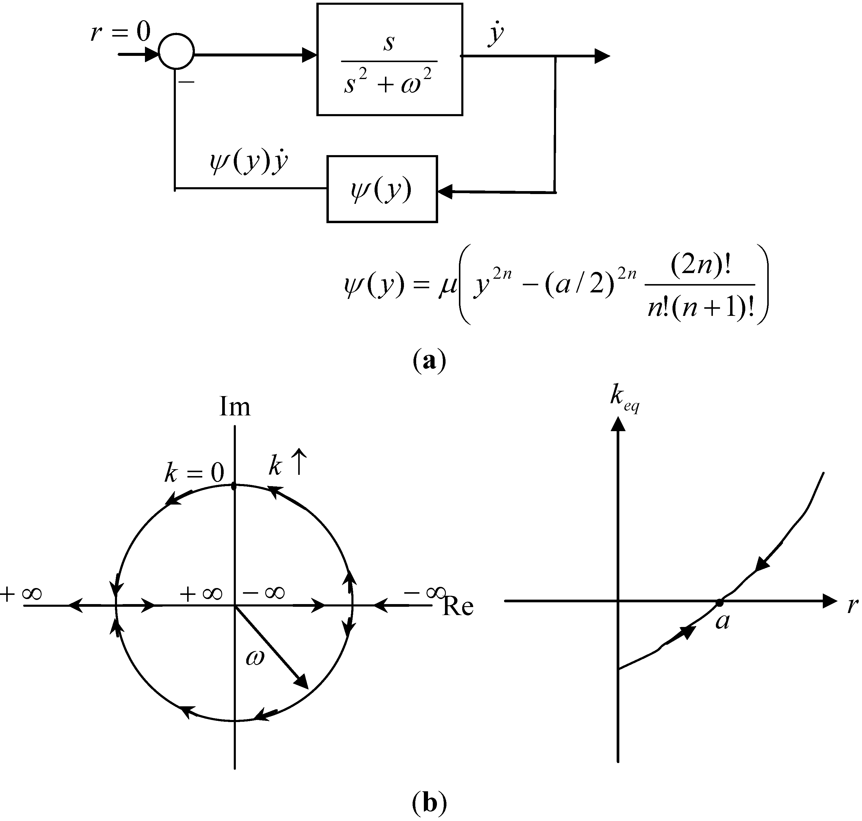
The HD-VDP dynamics in Equation (1) can be realized by a linear dynamics $G$ feedback-coupled with a $y$-dependent static gain $\mathrm{\psi }(y)$ as plotted in Figure 1a. The transfer-function of the linear dynamics $G$ is:

$$G(s)=\frac{s}{s^2+{\mathrm{\omega }}^2}$$

(3)

and the static gain is:

$$\mathrm{\psi }(y)=\mathrm{\mu }(y^{2n}-b); b=\frac{(2n)!}{n!(n+1)!}{\left(\frac{a}{2}\right)}^{2n}$$

(4)

wherein $s$ is the independent variable of the Laplace Transform. The nonlinearity $\mathrm{\psi }(y)$ is memory-free and can thus be represented as an equivalent gain $k_{eq}$ dependent merely on the amplitude of the HD-VDP output $y$, rather than the frequency $\mathrm{\omega }$. Based on the discipline of Describing Function, e.g., in [46], the equivalent gain of the nonlinear feedback in Figure 1a can be derived as follows.

In the polar-coordinated phase plane of $(y,\dot{y})$, set $y=r\cos \mathrm{\theta }$ and $\dot{y}=r\sin \mathrm{\theta }$, where the amplitude $r$ and the phase $\mathrm{\theta }$ are considered slowly time-variant. The nonlinear feedback in Figure 1a becomes:

$$\mathrm{\psi }(y)\dot{y}=\mathrm{\mu }r\sin \mathrm{\theta }(r^{2n}{\cos }^{2n}\mathrm{\theta }-b)\equiv c_0/2+c_1\cos \mathrm{\theta }+d_1\sin \mathrm{\theta }+c_2\cos \mathrm{\theta }+d_2\sin 2\mathrm{\theta }+\cdots , \mathrm{\theta }\in [-\mathrm{\pi },\mathrm{\pi }]$$

(5)

which has been expanded by Fourier series. Therein,

$$c_i=\frac{\mathrm{\mu }r}{\mathrm{\pi }}{\displaystyle {\int }_{-\mathrm{\pi }}^{\mathrm{\pi }}\cos i\mathrm{\theta }\cdot \sin \mathrm{\theta }(r^{2n}{\cos }^{2n}\mathrm{\theta }-b)d\mathrm{\theta }}=0, i=0,1,\cdots$$

(6)

$$d_i=\frac{\mathrm{\mu }r}{\mathrm{\pi }}{\displaystyle {\int }_{-\mathrm{\pi }}^{\mathrm{\pi }}\sin i\mathrm{\theta }\cdot \sin \mathrm{\theta }(r^{2n}{\cos }^{2n}\mathrm{\theta }-b)d\mathrm{\theta }} i=1,2,\cdots$$

(7)

It can be found by numerical calculation that those amplitudes of higher modes, $d_i$ for $i>1$, are significant smaller than $d_1$—the amplitude of the oscillation at the natural frequency $\mathrm{\omega }$ of the linear dynamics $G$. That is, the higher modes will be firstly filtered out of the loop by the single-degree vibrator $G$ in Equation (3) and later by the low-pass fitter in Equation (2).

Figure 1. Synthesis of HD-VDP oscillators. (a) Feedback representation of van der Pol oscillators; (b) Root Locus and Equivalent Gain.

Figure 1. Synthesis of HD-VDP oscillators. (a) Feedback representation of van der Pol oscillators; (b) Root Locus and Equivalent Gain.

Therefore, to a proper accuracy, the equivalent gain $k_{eq}(r)$ of the feedback gain $\mathrm{\psi }(y)$ is:

$$k_{eq}(r)=\frac{d_1}{r}$$

(8)

which, inferred from Equation (7), is time-variant in the sense of time-averaging over a cycle of oscillation. Explicitly:

$$k_{eq}=\frac{\mathrm{\mu }}{\mathrm{\pi }}{\displaystyle {\int }_{-\mathrm{\pi }}^{\mathrm{\pi }}{\sin }^2\mathrm{\theta }(r^{2n}{\cos }^{2n}\mathrm{\theta }-b)d\mathrm{\theta }}$$

(9)

That is,

$$\mathrm{\pi }\left(\frac{k_{eq}}{\mathrm{\mu }}+b\right)=r^{2n}{\displaystyle {\int }_{-\mathrm{\pi }}^{\mathrm{\pi }}{\cos }^{2n}\mathrm{\theta }-{\cos }^{2(n+1)}\mathrm{\theta }d\mathrm{\theta }}$$

(10)

Substituting the exponential expression of co-sinusoidal functions:

$${\cos }^m\mathrm{\theta }\equiv {\left(\frac{e^{j\mathrm{\theta }}+e^{-j\mathrm{\theta }}}{2}\right)}^m$$

(11)

into Equation (10) yields

$$\mathrm{\pi }\left(\frac{k_{eq}}{\mathrm{\mu }}+b\right)=2\mathrm{\pi }\cdot r^{2n}\cdot \left(\frac{1}{2^n}\frac{(2n)!}{n!n!}-\frac{1}{2^{n+2}}\frac{(2n+2)!}{(n+1)!(n+1)!}\right)$$

(12)

That is,

$$\begin{gathered} \frac{1}{2}\left(\frac{k_{eq}}{\mathrm{\mu }}+b\right)=r^{2n}\cdot \frac{1}{2^{2n+2}}\frac{(2n)!}{(n+1)!(n+1)!}\cdot \left(4{(n+1)}^2-(2n+1)(2n+2)\right) \\ =r^{2n}\cdot \frac{2n+2}{2^{2n+2}}\frac{(2n)!}{(n+1)!(n+1)!} \end{gathered}$$

(13)

Equation (13) can be further rephrased as:

$$\frac{k_{eq}}{\mathrm{\mu }}+b=r^{2n}\cdot \frac{n+1}{2^{2n}}\frac{(2n)!}{(n+1)!(n+1)!}=r^{2n}\cdot \frac{1}{2^{2n}}\frac{(2n)!}{n!(n+1)!}={\left(\frac{r}{2}\right)}^{2n}\frac{(2n)!}{n!(n+1)!}$$

(14)

As a result, the equivalent gain $k_{eq}$ is found to be:

$$\frac{k_{eq}}{\mathrm{\mu }}=\frac{2n!}{n!(n+1)!}\left[{\left(\frac{r}{2}\right)}^{2n}-{\left(\frac{a}{2}\right)}^{2n}\right]$$

(15)

In Figure 1b are plotted the root-locus of $1+kG(s)=0;G(s)=s/(s^2+{\mathrm{\omega }}^2)$ and the equivalent gain $k_{eq}$ versus the amplitude $r$. Let us tract the interaction between the closed-loop eigenvalues and the equivalent gain $k_{eq}$ of the nonlinear feedback until the dynamical equilibrium is reached. Suppose the initial amplitude is larger than $a$, the closed-loop eigenvalues start running at West Gauss, and hence the amplitude $r$ begins to decrease, which in turn reduces the equivalent gain $k_{eq}$, pushing the closed-loop eigenvalues toward East Gauss. However, eigenvalues being at East increases the amplitude $r$, and at the same time increases $k_{eq}$, which pulls the eigenvalues back to West Gauss. Conceptually back and forth, the closed-loop eigenvalues have to asymptotically stop at the equilibrium point on the imaginary axis corresponding to $k_{eq}=0$. This implies that the steady-state exhibits in limit-cycle with the amplitude $a$ and the (angular) frequency $\mathrm{\omega }$. Suppose the initial amplitude is smaller than $a$, by the same analysis, the close-loop eigenvalues evolve into the same equilibrium point, yielding the same sustained oscillation.

The transfer-function of the filter of Equation (2) is:

$$\frac{Z(s)}{Y(s)}=\frac{a^{-1}\sqrt{2}}{1+1/\mathrm{\omega }\cdot s}$$

(16)

the amplitude ratio of which from the HD-VDP output $y$ to the filtered output $z$ is the inverse of $a$ when $y$ is oscillated at the frequency $\mathrm{\omega }$. Therefore, the output of the frequency generator is normalized to one. Meanwhile, those higher modes implied by the nonlinear feedback are refined out of the loop through the low-pass filter of Equation (16).

The damping adjuster $\mathrm{\mu }$ indicates the strength of the damping, so increasing $\mathrm{\mu }$ will shorten the transience up to limit cycling. However, this enlarges the shift of the limit-cycle frequency way from the preset frequency $\mathrm{\omega }$. To remove such a trade-off between steady accuracy and transient dexterousness, we can reduce the damping adjuster $\mathrm{\mu }$, but increase the damping order $n$. This is the main advantage of the HD-VDP over the conventional VDP according to $n=1$ in [36].

3. DSP-Based Implementation of Signal Generators

By choosing three state variables: $x_1=y$, $x_2=\dot{y}$, and $x_3=z$, the state-space realization of the dynamics in Equations (1) and (2) becomes:

$$\begin{gathered} u=-\mathrm{\mu }\left(x_1^{2n}-{(a/2)}^{2n}\frac{(2n)!}{n!(n+1)!}\right)x_2 \\ \left[\begin{array}{c}{\dot{x}}_1\\ {\dot{x}}_2\\ {\dot{x}}_3\end{array}\right]=\left[\begin{array}{ccc}0& 1& 0\\ -{\mathrm{\omega }}^2& 0& 0\\ a^{-1}\sqrt{2}\mathrm{\omega }& 0& -\mathrm{\omega }\end{array}\right]\left[\begin{array}{c}{x}_1\\ x_2\\ x_3\end{array}\right]+\left[\begin{array}{c}0\\ 1\\ 0\end{array}\right]u. \\ z=\left[\begin{array}{ccc}0& 0& 1\end{array}\right]\left[\begin{array}{c}{x}_1\\ x_2\\ x_3\end{array}\right] \end{gathered}$$

(17)

It appears as a feedback-interconnected form: $u=f(x;\mathrm{\mu },a)$; $\dot{x}=A(\mathrm{\omega },a)x+Bu$; $z=Cx$, where the preset frequency $\mathrm{\omega }$, the pre-scaling amplitude $a$, the damping adjuster $\mathrm{\mu }$, and the damping order $n$ constitute the time-varying parameter that can be on-line scheduled in a time-averaging fashion.

The frequency modulator in Equation (17) is then implemented into a dsPIC chip with the Euler discretization as follows. Continuous-to-digital conversion of Equation (17) yields:

$$\begin{array}{l}{u}_k=f(x_k;{\mathrm{\mu }}_j,a_j)\\ x_{k+1}=\mathrm{\Phi }({\mathrm{\omega }}_j,a_j)x_k+\mathrm{\Gamma }({\mathrm{\omega }}_j,a_j)u_k\\ y_k=C{x}_k\end{array}$$

(18)

where $k$ and $j$ are fast-time and slow-time sampling indexes, respectively. The system matrices $(\mathrm{\Phi },\mathrm{\Gamma })$ can be on-line calculated in a slow-time fashion; explicitly,

$$\begin{gathered} \mathrm{\Phi }({\mathrm{\omega }}_j,a_j)=e^{A({\mathrm{\omega }}_j,a_j)}\approx {\displaystyle \sum _{i=0}^N\frac{A^i({\mathrm{\omega }}_j,a_j)T^i}{i!}} \\ \mathrm{\Gamma }({\mathrm{\omega }}_j,a_j)\approx T{\displaystyle \sum _{i=1}^n\frac{A^{i-1}({\mathrm{\omega }}_j,a_j)T^{i-1}}{i!}} \end{gathered}$$

(19)

where $T$ is the fast-time sampling period that is short enough to make the above Taylor-series expansion accurate even with few terms, say, $N=2$ or $3$ as $T$ is $0.001$ second.

At the present time $t_k$ the dsPIC merely stores the current state $x_k$, and the update of state from $x_k$ to $x_{k+1}$ at next instant is fulfilled by the DSP-engine performing addition and multiplication of floating numbers according to Equation (18). In the sense, any time can be treated as the initial time, which makes the real-time processing best efficient. Moreover, the intervals of state update are held identical to those in computer simulation, so that the real-timed operation matches the dynamics that has been verified by off-line calculation, thus achieving robust implementation. At any instance, a pulse-width modulated (PWM) signal in line with the output $y$ is sent to the gate-driving circuit of the switched power converter that drives the photo valve.

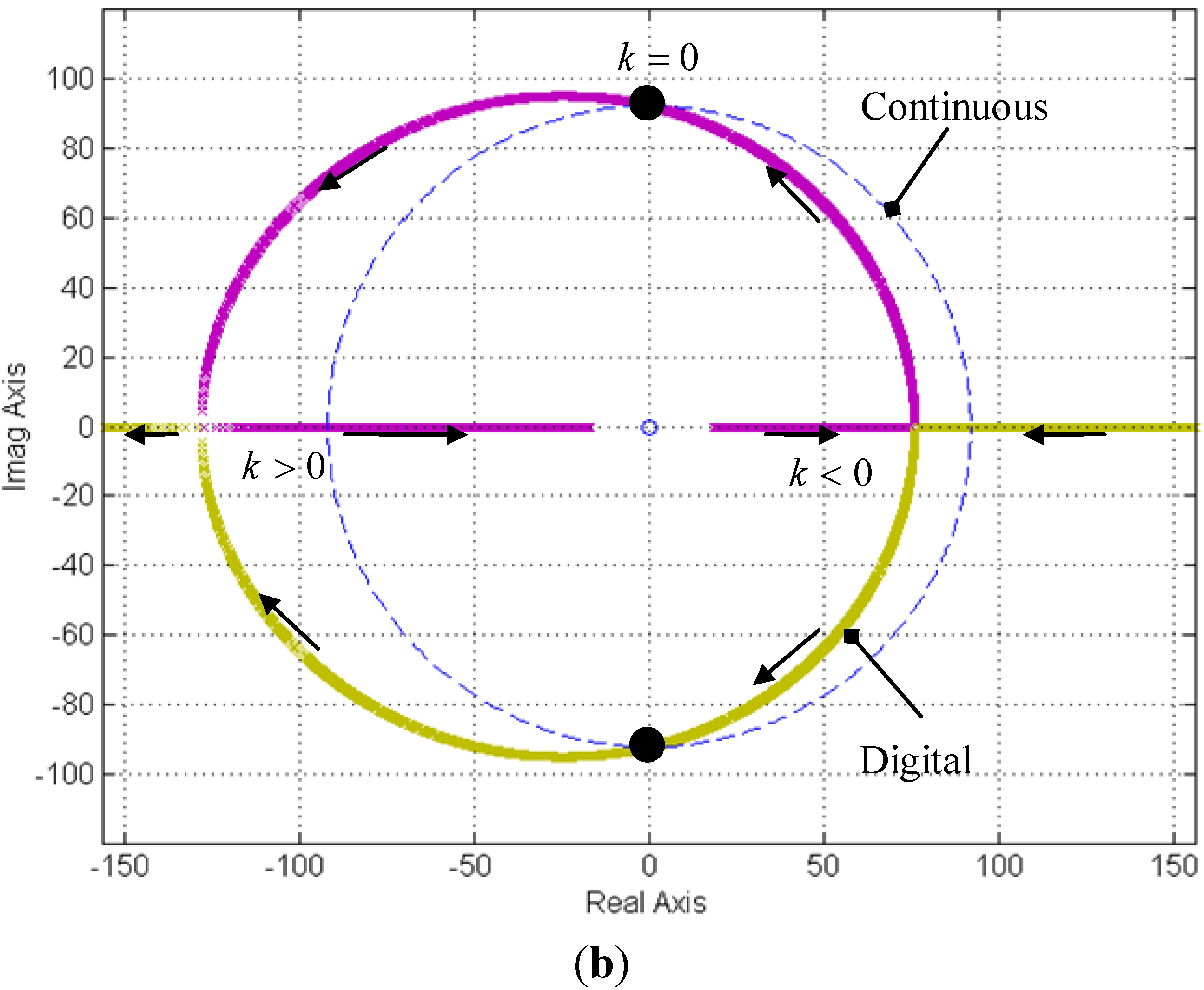
Figure 2 records the performance of the digital-signal-processing (DSP)-based HD-VDP frequency modulator, which visualizes the accuracy in frequency and the real-time fashion of frequency modulation with the second-order damping $n=2$. As shown in Figure 2, the limit-cycling frequency and amplitude of the digital HD-VDP out of temporal discretization are accurately kept at those of the continuous HD-VDP. This fact can be investigated through the Root Locus of:

$$\tilde{G}(s)=\frac{s}{s^2+{\mathrm{\omega }}^2}\cdot e^{-\frac{T}{2}s}$$

(20)

where the sampling time $T$ virtually arouses $T/2$ time-delay from the zero-order holding (ZOH) in digital signal processing, as shown in Figure 3a. Figure 3b shows its dominated root-locus for the case: $\mathrm{\omega }=14.64\times 2\mathrm{\pi }$ and $T=0.005$.

Figure 2. Frequency-modulation with the DSP-based HD-VDP signal generator.

Figure 2. Frequency-modulation with the DSP-based HD-VDP signal generator.

Figure 3. Topological analyses upon temporal discretization. (a) Time-delay effect due to zero-order holding; (b) Root Locus of 1 + kG(s)$e^{-\frac{T}{2}s}$.

Figure 3. Topological analyses upon temporal discretization. (a) Time-delay effect due to zero-order holding; (b) Root Locus of 1 + kG(s)$e^{-\frac{T}{2}s}$.

As shown in Figure 3b, the dominated root-locus of the discretized version $\tilde{G}$ is stretched to an ellipse from the circle of the continuous version $G$ and moved left by the ZOH-implied time-delay. Fortunately, both are topologically equivalent in the sense that one can be obtained from the other merely by scaling and shifting, and their equilibrium points $(\mathrm{\omega },k)$ coincide with each other in the imaginary axis. Therefore, the digital HD-VDP is asymptotically equivalent to the continuous HD-VDP, in both of which limit-cycling frequencies and amplitudes will be identical even beyond a reasonable range of sampling speeds. In this case, the dominated root-locus of the digital version begins to diverge from the topology of the continuous root-locus as the sampling time $T$ approaches 15% of the oscillation period. Then the asymptotical behavior of the digital HD-VDP becomes unpredictable; it often appears as instability or asymptotical stability, rather than limit cycling.

4. Frequency-Domain Identification

Modified from that in Hong and Chou [1], the thermoacoustic solar-power generator is designed as in Figure 4. It is assembled by the alternative current generator, the acoustic resonator, the thermal storage, and the photo valve that consumes very little power on switching. At the head end of the resonator, the heat-flux resulting from sunlight gives rise to the entropy rate that changes the fluid density there, which in turns initiates acoustic velocity. Therein, the heat-flux excitation expanding and contracting the fluid acts as a source of acoustic wave that rides on the working gas and arrives at the load end to push and pull the piston, generating AC electricity. A frequency controller comes to online keep the switching of the photo valve at the most powerful natural-frequency, which drives standing waves up to resonance and thus increases mechanical power enormously.

Figure 4. Active thermoacoustic solar-power generators.

Figure 4. Active thermoacoustic solar-power generators.

The thermoacoustic engine behaves like a heat-driven Webster’s horn, which takes the acoustic velocity $u_0$ sourced from the heat-flux excitation $q$ at the head end and drives the piston at the tail end. Therein the source velocity $u_0$ is:

$$u_0=\frac{\mathrm{\gamma }-1}{\mathrm{\gamma }}\frac{q}{P}$$

(21)

where $P$ stands for the ambient pressure and $\mathrm{\gamma }$ for the specific heat-ratio of the working gas, both of which are design parameters.

As an example, let the solar heat-flux excitation be $q=500$ W/m², the length of resonator be $3$m, the projection area of the reflector be 7 m², the working gas be the air, and the ambient pressure be the atmosphere. Then the HD-VDP frequency generator in Section 2 is put into work on the system identification in frequency domain. The identified data is collected into Figure 5—a pair of bode plots, which shows the perturbed amplitude of the head pressure $p_0/P$ and its phase difference $\mathrm{\theta }$ with the head velocity $u_0$, versus the switching (angular) frequency of the photo valve. Known from the principle of AC power, the real power is

$$POW=\widehat{u}\widehat{p}\cos \mathrm{\theta }\cdot \mathrm{\beta }$$

(22)

where $\widehat{u}$ and $\widehat{p}$ are the root-mean-square values of $u_0$ and $p_0$, respectively, $\cos \mathrm{\theta }$ acts as the power factor, and $\mathrm{\beta }$ is the coefficient of flow leakage [1].

From the Figure 5, the advantage of resonance upon power ratings can easily be observed. A frequency modulator is thus necessary to online keep the photo valve at the most powerful resonant-frequency. For robustness and accuracy, such a frequency modulator should be a feedback controller. In the next section, we extend the methodology of the HD-VDP presented in Section 4 into the principle of Dynamical Equilibrium for synthesizing such a feedback controller.

Figure 5. System identification in frequency domain.

Figure 5. System identification in frequency domain.

5. The Principle of Dynamical Equilibrium

As an instructional example, let us consider the feedback loop of Figure 6a, wherein the linear time-invariant dynamics $G(s)$ (with memory) is feedback-coupled with the saturation as an example of static nonlinearity $u=\mathrm{\psi }(e)$ (without memory). Figure 6b plots the root-locus of the linear dynamics $G(s)$, $1+kG(s)=0$, and the approximated gain of the static nonlinearity $\mathrm{\psi }$, $\widehat{k}\equiv u/e$. Therein, the triple $(k_i,{\mathrm{\omega }}_i,e_i)$, $i=1,2$, denotes that the root-locus crosses the imaginary axis at $(0,\pm j{\mathrm{\omega }}_i$) as $\widehat{k}=k_i$ to which the corresponding value of $e_i$ is known from the right-side diagram of Figure 6b. The temporal response of the input $e$ to the nonlinearity $\mathrm{\psi }$ is affected by the closed-loop eigenvalues that are online moved along the root locus by the positive gain $\widehat{k}=u/e$, which in turn determines the response of the input $e$. Therefore, the interaction between the closed-loop eigenvalues and the $e$-dependent feedback-gain determines whether the closed-loop of Figure 6a exhibits in asymptotical stability, limit cycling, or instability. This is called here Dynamical Equilibrium.

Let $e_0$ denote the initial value of the input $e$, and define the saturation-gain $k_{sat}$ by $u_{sat}/e_{sat}$. In the sequel is the detailed presentation of the principle of Dynamical Equilibrium.

(I) $k_{sat}>k_2$

(1) $e_0<e_2$: As shown in Figure 6b, the dominated eigenvalues of the closed-loop are initially located in East Gauss- the unstable region. The amplitude of $e$ begins to increase, and thus the feedback gain $\widehat{k}$ of the nonlinearity decreases in the meanwhile, which in turn moves west the closed-loop eigenvalues along the root-locus of $G(s)$. As the root-locus crosses the imaginary axis onto West Gauss—the stable region, the feedback-gain $\widehat{k}$ tends to increase since the $e$-amplitude is decreasing, which in turn moves east the closed-loop eigenvalues $p$. Therefore, the closed-loop eigenvalues are forced to stop at $(0,\pm j{\mathrm{\omega }}_2)$—the equilibrium points.

That is, the input $e$ will asymptotically behave sustained oscillation as a limit cycle with frequency ${\mathrm{\omega }}_2$. As for the amplitude $a$ of this limit cycle, it will be close to $u_{sat}/k_2$, but the exact value has to be calculated by the discipline of Describing Function, similarly as shown in Section 2. If the saturation degenerates into a relay, corresponding to $e_{sat}=0$, the $e$-amplitude is $(4/\mathrm{\pi })\times (u_{sat}/k_2)$ rather than $u_{sat}/k_2$. That is, the equivalent gain $k_{eq}$ of the relay nonlinearity is $(4/\mathrm{\pi })\times u_{sat}$ over the limit-cycle amplitude, the value of which is especially accurate for low-passed $G$ or powerful actuation.

Figure 6. Dynamical Equilibrium Approach. (a) An example to study Dynamical Equilibrium; (b) Limited cycle and unstable cases; (c) Asymptotically stable case.

Figure 6. Dynamical Equilibrium Approach. (a) An example to study Dynamical Equilibrium; (b) Limited cycle and unstable cases; (c) Asymptotically stable case.

(2) $e_2<e_0<e_1$: By a similar deduction, the closed-loop will asymptotically exhibit in limit-cycle with the frequency and amplitude identical with those of Case (I)-(1).

(3) $e_0>e_1$: A pair of closed-loop eigenvalues starts running at East Gauss. They move in the direction that the equivalent gain $k_{eq}$ increases, so the closed-loop poles have no chances to cross the imaginary axis. Thus the closed-loop system is unstable.

(II) $k_2>k_{sat}>k_1$

(1) $e_0<e_1$: As shown in Figure 6c, the dominated poles start running in West Gauss, and thus move in the direction that the equivalent gain $k_{eq}$ increases without possibility of arriving at East Gauss. The closed-loop system is thus asymptotically stable. Moreover, the dominated poles will stop at the locations associated with $k=k_{sat}$, which specify the approximated performance in terms of $\mathrm{\theta }$, $\text{σ}$ and ${\mathrm{\omega }}_n$ as shown in Figure 6c. Therein, the damping ratio is approximated by $\sin \mathrm{\theta }$, the rising time is by $1.8/{\mathrm{\omega }}_n$, and the settling time is by $4.6/\text{σ}$.

(2) $e_0>e_1$: By similar analysis, the closed-loop system is to be unstable.

(III) $k_{sat}<k_1$

The closed-loop eigenvalues always stays in East Gauss, thus the closed-loop system is unstable.

Summarily, the main idea of Dynamical Equilibrium is to tract the interaction between the closed-loop eigenvalues and the equivalent gain of the static feedback until the dynamical equilibrium is reached. In conjunction with the discipline of Describing Function, the amplitude and frequency of limit cycle, if any, can be accurately figured out. Moreover, the principle of Dynamical Equilibrium reveals that the initial trigger also affects the asymptotical behavior, which can be stability, limit-cycle or instability.

6. Synthesis of Feedback Control

For robust power-amplification at resonance anytime, a sensor is installed to online monitor the acoustic pressure at the head end of the resonator. The sensor’s output signals are transported to the feedback controller. Such a feedback-controller plays as a plant-in-loop frequency modulator that generates resonant signals to keep the photo-valve switched at the most powerful frequency. Moreover, it will parametrically be gain-scheduled by the working temperature in real operation.

In the feedback synthesis, the photo valve functions as a relay nonlinearly with the equivalent gain being $4q_{sat}/\mathrm{\pi }r$, where $r$ is the limit-cycle amplitude and $q_{sat}$ is the present heat-flux excitation. For the feedback synthesis and DSP-based implementation, the thermoacoustic dynamics [1] under control is made dimensionless by:

$$\tilde{p}\to \tilde{p}/{\tilde{p}}_0, \tilde{T}\to \tilde{T}/{\tilde{T}}_0, A\to A/A_0, \mathrm{\kappa }\to \mathrm{\kappa }/\mathrm{\gamma }R{\tilde{T}}_0$$

(23)

where ${\tilde{p}}_0$, ${\tilde{T}}_0$ and $A_0$ stand for the pressure, the temperature and the effective cross-section area at the head end, respectively, and $\mathrm{\kappa }$ for the compressibility of working gas. The independent and dependent variables are made dimensionless by:

$$t\to c_{0}t/\ell (c_0\equiv \sqrt{\mathrm{\gamma }R{\tilde{T}}_0}), x\to x/\ell , \mathrm{\psi }\to \frac{\mathrm{\psi }}{(\ell /c_0){\tilde{p}}_0}$$

(24)

where $\ell$ is the length of the acoustic resonator, and $c_0$ is the reference speed of sound. The dimensionless time, the longitudinal coordinate, and the Rayleigh’s displacement are denoted by $t$, $x$ and $\mathrm{\psi }$, respectively. The heat-flux excitation $q$ at the head end and the piston speed $v$ at the tail end are made dimensionless by:

$$q\to \frac{(\mathrm{\gamma }-1)\ell }{c_0{\tilde{p}}_0}q, v\to \frac{v}{c_0}$$

(25)

As a result, the non-dimensional dynamics of the entire engine has the same form as the original dynamics [1].

As shown in Figure 7, the entire dynamics has been represented by the thermoacoustic dynamics coupled with the internal feedback of load dynamics and the external feedback of control dynamics. Referring to Figure 7, let the plant $G$ denote the thermoacoustic dynamics internally feedback-coupled with the load dynamics, and let the to-be-synthesized feedback dynamics denoted by $K$.

Figure 7. Feedback-representation for the entire dynamics.

Figure 7. Feedback-representation for the entire dynamics.

At first, the feedback synthesis is guided by the Rayleigh criterion for thermoacoustic engines [1]:

$${\dot{E}}_T=A_0\frac{(\mathrm{\gamma }-1)q}{\mathrm{\gamma }P}{p}_0-{\mathrm{\beta }}^{-1}{A}_{\ell }v{p}_{\ell }$$

(26)

where the $E_T$ stands for the mechanical energy of the thermoacoustic vibration. Based on this criterion, if the feedback dynamics $K$ is as simple as a positive constant-gain, then the in-phase between the acoustic pressure and the heat fluctuation at the lead end leads the dynamics away from asymptotical stability. In conjunction with the relay constraint from the photo-valve switching, the engine tends to limit-cycle oscillation.

If the sunlight is strong enough, such a simple Rayleigh-based feedback is capable of sustained power generation. However, this encounters four aspects of difficulty:

(D1)

With the load dynamics, the oscillation frequency is usually away from the resonant frequency, which decreases the acoustic pressure and the power factor, thus restraining power amplification.

(D2)

The oscillation of the closed-loop will comprise multiple frequencies, causing engine knocks.

(D3)

Unavoidable uncertainties usually happen in modelling, which decentralize the performance of feedback control.

(D4)

In real operation, the thermoacoustic dynamics is parametrically dependent on the working temperature, with which the constant feedback-gain is unable to deal.

For the difficulty (D1), an East-Gauss zero is added into the feedback transfer-function to adjust the location of the equilibrium point on the imaginary axis, so that the limit-cycle frequency is pitched to the damped natural-frequency. Here we choose the Pade’s first-order approximation of time delay as the nominal feedback $K_0$:

$$K_0(s)=\frac{1-\mathrm{\tau }/2\cdot s}{1+\mathrm{\tau }/2\cdot s}$$

(27)

which provides the zero $z=$ $2/\mathrm{\tau }$ in East Gauss.

As for the difficulty (D2), we apply the technique of loop shifting to guarantee single-frequency resonance, as explained by the Figure 8 and the following texts thereupon. Firstly, decompose the plant dynamics $G$ into a nominated dynamics $G_0$ plus the residual dynamics $R_0$:

$$G=G_0+R_0$$

(28)

where $G_0$ comprises the dynamics of the most powerful mode within the effective frequencies of photo-valve switching, and $R_0$ contains the dynamics of the other modes. Secondly, adjust the value of $\mathrm{\tau }$ of $K_0$ to numerically obtain a satisfactory root-locus of $1-k{K}_0(s)G_0(s)=0$, wherein the equilibrium pitches to the most powerful frequency. Thirdly, let the feedback dynamics $K$ be the dynamics $K_0$ feedback-coupled with the relay function in series with the estimation of the residual dynamics $R$, as shown in Figure 8b. In the case that the estimated residual $R$ is coincidental to the real residual $R_0$, the entire dynamics in Figure 8b is identical to that of Figure 8a, which thus guarantees sustained power generation at single resonance of the most powerful mode. The resulting feedback dynamics is of high order, so we can program it into a dsPIC chip to take advantage of the DSP-engine therein. It online generates switching signals to the power converter that drives the photo valve.

However, the estimated residual $R$ is unusually identical to the real residual $R_0$, which arouses the difficulty (D3). To this, we need to perform a robust analysis to assess the affordable sizes of uncertainty. Let the dynamics of Figure 8b be equivalently represented by Figure 8c. Following the signal flow, one can reorganize the dynamics of Figure 8c into the equivalent feedback-connection between the generalized plant $M$ and the relay function, as shown in Figure 8d. Therein, the generalized plant $M$ is:

$$M=K_0{G}_0+K_0(R_0-R)$$

(29)

Secondly, investigate whether the generalized root-locus of $1-kM(s)=0$ is topologically close to the nominal root-locus of $1-k{K}_0(s)G_0(s)=0$.

Figure 8. Synthesis of feedback frequency modulator. (a) Dominated feedback; (b) Loop Shifting ; (c) Dynamical equivalence to (b); (d) Robust analysis.

Figure 8. Synthesis of feedback frequency modulator. (a) Dominated feedback; (b) Loop Shifting ; (c) Dynamical equivalence to (b); (d) Robust analysis.

Figure 9 plots the root-locus of $1-kM(s)=0$ when the real residual $R_0$ is perfectly estimated by $R$. Due to pole-zero cancellation in West Gauss, this root-locus is topologically identical to the nominal root-locus, thus keeping the same power amplification. Figure 10 plots the generalized root-locus when the estimation of the residual dynamics has 7% discrepancy in the natural frequencies. As indicated by Figure 10, its topology is very close to the nominal one from the viewpoint of Dynamical Equilibrium in Section 5. From the equilibrium points of the other modes, we can still infer that the asymptotical oscillation has tiny components of some other modes, other than the most powerful mode. Figure 11 records the temporal responses of the acoustic pressures at the tail end of the acoustic resonator, with uncertainties of $0\%$, 5% and 7%, respectively. The engine knocks are unobservable from Figure 11, thus the high-order feedback from the loop-shifting should work well in practice. In fact, a tiny engine knock still exists in practice, which is detectable from the close view of Figure 11, as shown in Figure 12.

To deal with the difficulty (D4), thermal couples are installed inside the resonator to online measure the working temperature, by which the nominated feedback $K_0$ and the estimated residual $R$ are online gain-scheduled. This keeps resonance even in the transience of temperature variations. The set of feedback dynamics to the difficulties (D1)–(D3) at a matrix of temperatures is stored in the dsPIC chip for the purpose of gain-scheduling in a real-time fashion. As a final verification, the thermoacoustic solar-power generator is put to experiments in lab with the working temperature being controlled. 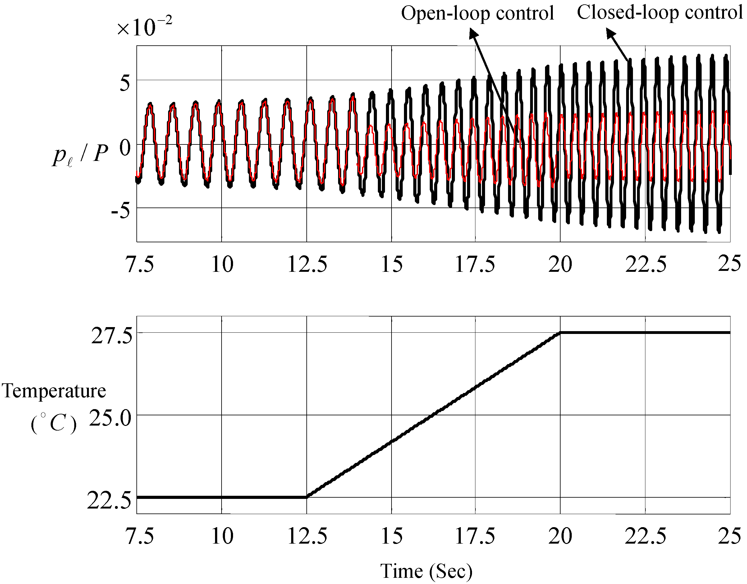Figure 13 records the responses under the feedback control and the open-loop VDP control, when the working temperature is slowly time-variant from 22.5 to 27.5 °C. Figure 13 clearly illustrates the benefits of applying the strategy of feedback control. That is, the conventional resonance can be generalized into the transient resonance by the feedback frequency-modulation.

Figure 9. The Root locus of generalized plant $M$, $R=R_0$.

Figure 9. The Root locus of generalized plant $M$, $R=R_0$.

Figure 10. The Root locus of generalized plant $M$, ${\mathrm{\Delta }}_{\mathrm{\omega }}=7\%$.

Figure 10. The Root locus of generalized plant $M$, ${\mathrm{\Delta }}_{\mathrm{\omega }}=7\%$.

Figure 11. Temporal responses under temperature uncertainties.

Figure 11. Temporal responses under temperature uncertainties.

Figure 12. Close view of Figure 11.

Figure 12. Close view of Figure 11.

Figure 13. Measured temporal responses under time-variant temperature.

Figure 13. Measured temporal responses under time-variant temperature.

Currently, we are taking the polymer dispersed liquid crystal (PDLC) as the photo valve in performing system identification and feedback control, which consumes less than 5 W/m², very little in comparison with the power harvested. Combined with power driver, it costs less than one hundred dollars per square meter. As shown in the Figure 4, the thermoacoustic engine developed here needs much less area of PDLC than the previous design in [1]. Furthermore, one acoustic-pressure sensor is implemented in the head end of the resonator for feedback control, and a thermal couple is in the middle for gain-scheduling the controller. Roughly speaking, for a 3 m-long thermoacoustic engine, the ambient pressure is better ranged from 0.45 to 1.0 atm, and the heal-flux should be more than 200 W/m² to achieve a proper working-temperature, ranged from 15 to 40 °C.

For further study on the active design on thermoacoustic engines, we also record the following findings:

(1)

In normal summer of southern Taiwan, a 3 m-long engine needs almost 10 min before reaching the asymptotic operation. After that, the feedback controller can automatically adjust the engine at the maximum power-rating in a real-time fashion.

(2)

Smaller engines are more power-efficient and need less time to reach resonance.

(3)

In the 3 m-long engine, as the amplitude of acoustic vibration exceeds almost 20% of the environmental pressure, acoustic behavior begins to disappear and mean-flow fluctuation is instead observed. Moreover, this situation is getting apparent along with engine length.

(4)

For the present, the efficient switching frequencies of available photo-valves are less than 100 Hz, so that the engine size cannot be as small as best, which limits the power efficiency.

7. Conclusions

In convention, the resonance was merely considered for steady-state behavior. Via feedback control, this paper extends the conventional resonance into the resonance for transient oscillation. For sustained power-amplification, the present design applies the transient resonance to keep the thermoacoustic solar-power generators at resonance anytime in real operation. In advance of the controller design, the higher-damped van-der-Pol oscillator is created as an improved frequency generator for system identification in frequency domain. Both the signal generator for frequency-domain identification and the feedback controller for online operation are synthesized with the principle of Dynamical Equilibrium newly developed in this paper. The frequency-domain identification makes possible to modify the mathematical modelling and identify the most powerful mode. The developed controller is observed to robustly operate the engine always at the maximum power-rating.