1. Introduction
In recent years, people have been paying more and more attention to developing renewable energy resources due to the serious global energy shortage and environmental issues. With the development of distribution technology, the microgrid concept [
1,
2,
3] provides an effective way for the comprehensive utilization of renewable energy and other distributed generation (DG).
Electric vehicles (EVs) have lower pollutant emissions and lower carbon dioxide emissions than conventional vehicles. Although conventional vehicles are more competitive in terms of cost at present, the cost of EVs will be gradually reduced with the development of vehicle storage battery technology and rising fossil fuel prices, making EVs more and more competitive. A large number of EVs charging in the power grid is bound to cause many challenging issues, not only increasing the burden of grid peak load, but also affecting the system voltage and frequency [
4,
5]. With the proposed vehicle-to-grid (V2G) concept [
6], these problems might be alleviated. V2G technology allows bidirectional power flow between the grid and the electric vehicle’s battery. EVs can thus not only purchase power from the power grid but also feed power back to the grid as distributed energy resources through connection devices while they are idle. Therefore, integrating EVs into the microgrid system, through charging and discharging control strategies, one can achieve peak load shifting and improve the economics of the system [
7,
8,
9,
10].
Economic dispatch is a basic problem of microgrid system operation. Dynamic economic dispatch takes the microgrid as a discrete time system, and is generally minute-level optimization. Normally, it is solved by dividing the dispatch cycle into small time intervals of 1 minute or 5 minutes, and then a static economic dispatch is employed to solve the problem in each interval [
11]. This takes the coordination of the adjacent scheduling periods into account. Therefore it is more in accordance with the actual microgrid system operation. Since multi-objective dispatch was first introduced, there have been many studies choosing objective functions, considering not only operating cost but also environmental benefit, and the dispatch algorithm is multiple [
12,
13,
14,
15,
16,
17]. There are the lowest fuel cost, minimum SO
2 emissions, minimum NO
x emissions in [
14], but in terms of pollution, SO
2 and NO
x can be a unified consideration. Taking the reduction in greenhouse emissions into account, CO
2 emissions should be considered as one of the objective functions, but in [
15], CO
2 emissions was considered together with the pollutant emissions. That is improper. NSGA-II is employed in [
14] and [
16], and the performance of the algorithm is good. But NSGA-II can only be employed to solve a single period of scheduling, while dynamic dispatch needs to coordinate adjacent periods, so it does not apply. The method in [
17] also has this problem.
Therefore, this paper establishes a microgrid system which includes wind turbines (WTs), photovoltaic arrays (PVs), diesel engines (DEs), fuel cells (FCs), a storage battery (BS) and plug-in EVs. On the basis of mathematical models of EVs, considering the operating cost, pollutant treatment cost and carbon dioxide emissions as the dispatch objective functions of the microgrid system, this paper uses the judgment matrix method to convert the multi-objective functions to a single objective function, then uses an improved particle swarm algorithm (PSO) to simulate an example of the microgrid system’s economic dispatch, including V2G under different operation control strategies. We discuss the impact of EVs under different charging and discharging modes on the results of dynamic economic dispatch, and the impact of the load fluctuation. The simulation results verify the validity of the models and strategies.
2. The Load Models of Electric Vehicles
2.1. Spatial and Temporal Characteristics of EVs
In this paper, the modeling of EVs is intended primarily for household plug-in hybrid EVs. Spatial characteristics take the owner’s driving habits into account, simply understood as the daily mileage problem. Temporal characteristics are mainly on account of the end time of driving; assuming that owners start charging after the end of travel, this time can be regarded as the charging start time. According to statistics in [
18], the daily mileage of EVs
S approximately meets the lognormal distribution, for which the probability density function is:
Also in [
18], the end time of EVs driving
t0 approximately meets a normal distribution, for which the probability density function is:
where
;
;
;
.
Each EV is charging and discharging under conventional slow mode. The daily mileage of EVs can be obtained from Equation (1), while the end time of EVs’ driving, which is the charging start time, can be obtained from Equation (2).
2.2. The Load Model under Autonomous Charging Mode
The autonomous charging mode of EVs is the case where owners start charging their EVs just according to their own convenience, without relevant government policies, and this mainly concerns EVs which cannot be involved in scheduling. The power flow is unidirectional from the power grid to the EVs. The earliest possible time that the EVs can be recharged depends on the time when people arrive home after the last trip of the day. The charging duration of each EV can be obtained from the following equation:
where
is the power consumption per hundred kilometers in kWh/100 km;
is charging power of EVs in kW;
is the charging efficiency of EVs.
For each EV, the end time of charging
Tend can be obtained from the charging start time
Tstart and the charging duration. Then by accumulating the charging power of each period, we can get the total charging load
PEVload(
t). Because EVs charging periods are independent of each other, we can calculate the daily load profile of a large number of EVs charging, which is as follows:
where
N is the total number of EVs;
Pi(
t) is the charging power of the EV;
i is the period
t in kW;
CEV is the capacity of EV battery in kWh;
PdisC is the discharging power of EVs in kW.
2.3. The Load Model under Coordinated Charging and Discharging Mode
The EV coordinated charging and discharging mode, which can also be described as V2G, is intended to control EVs charging and discharging in an orderly and centralized way, considering guidance on electricity pricing policy and owners’ behavior. This section focuses on grid-connected EVs which can be scheduled. For the convenience of this study, it is assumed that these EVs can be completely scheduled. During off-peak load periods, EVs are charging as load. During peak load periods which may involve several hours around the load peak within 1 day, EVs are discharging as power sources.
From the EV battery state of charge (SOC) constraints, daily mileage and discharging power, we can get the maximum discharging duration:
The discharging start time Tstart_disC is determined by the end time of EV driving and the peak load periods. The end time of discharging Tend_disC is determined by the maximum discharging duration and dispatch cycle, the deadline for which is 24:00. Tend_disC minus Tstart_disC gets the actual discharging time TdisC. During that time, the EVs are discharging. Then by accumulating the discharging power of each period, we can get the total discharging power within the discharging periods.
The power demand of EV charging is equal to the total power consumption within one day, including daily travel consumption and discharging capacity.
Then we can get the charging duration:
Then, using Equation (4) to accumulate the charging power, we can get the total charging load of EVs.
2.4. The Computational Flowchart of the Daily Load of EVs
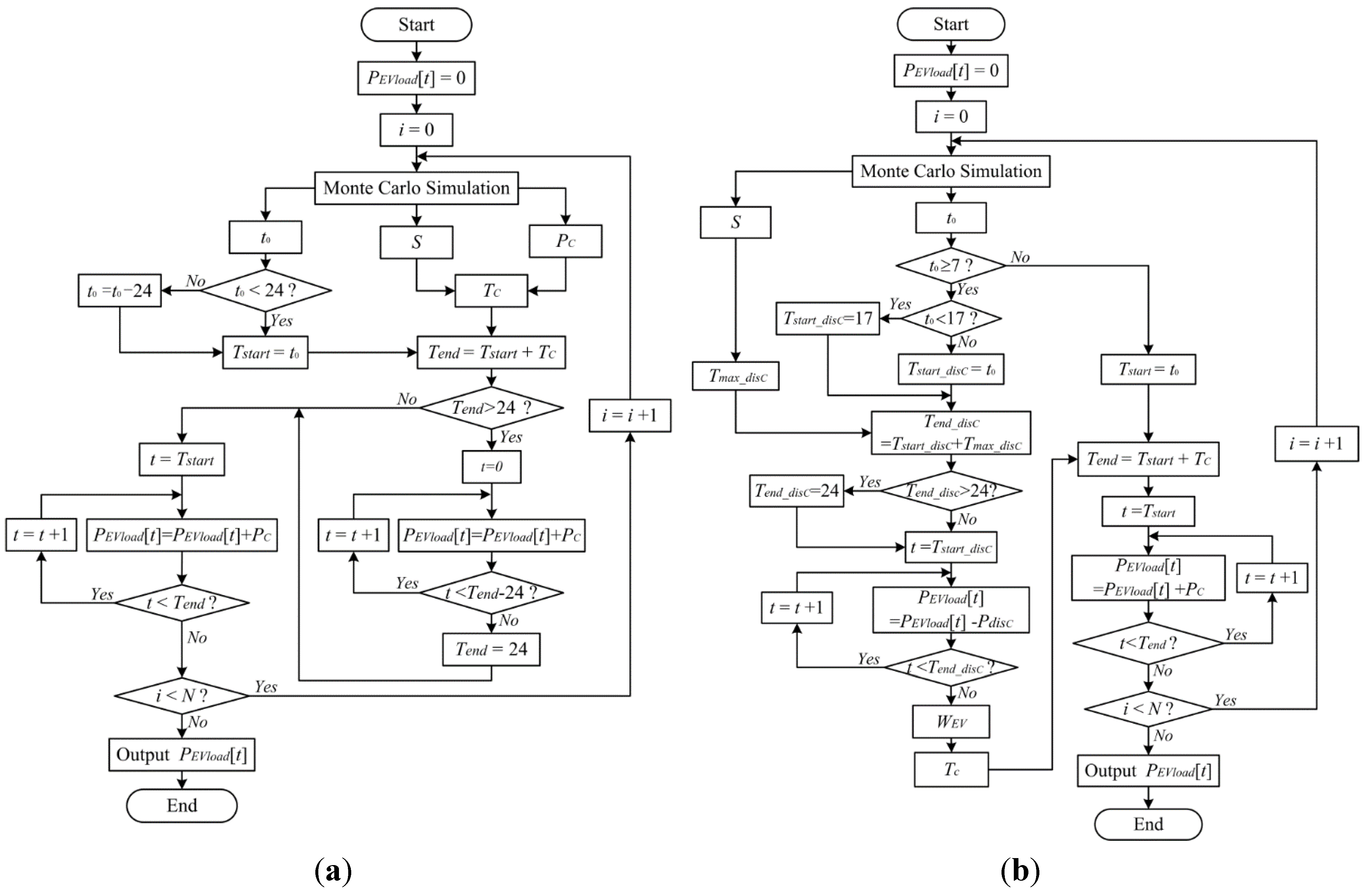
Figure 1 shows the computational flowchart of the daily load of EVs. The time is in hours.
Figure 1.
(a) The computational flowchart of the daily load of EVs under autonomous charging mode; (b) The computational flowchart of the daily load of EVs under coordinated charging/discharging mode.
Figure 1.
(a) The computational flowchart of the daily load of EVs under autonomous charging mode; (b) The computational flowchart of the daily load of EVs under coordinated charging/discharging mode.
3. Multi-Objective Functions Modeling of Microgrid System
3.1. Multi-Objective Functions of the Microgrid System
The mathematical model of multi-objective optimization which has
n-dimensional decision variables can be described as follows:
where
is
n-dimensional decision variables;
is the
k-th objective function;
is inequality constraints; and
is equality constraints.
In this paper, three objective functions of microgrid system economic dispatch are considered: the lowest operating cost, the lowest pollutant treatment cost, and the least carbon dioxide emissions:
(1) Objective function 1: the lowest operating cost
For the microgrid, the operating cost
of the system can be described as follows:
where
CFuel is the fuel consumption cost of the DGs in ¥;
COM is the operating and management cost of the DGs in ¥;
CGrid is the cost of interaction between microgrid and power grid;
CLS is the compensation expense of interruptible load in ¥;
M indicates whether the microgrid connects with the grid or not. When the microgrid is connected with the power grid,
M = 1; when the microgrid is in island mode,
M = 0.
The depreciation cost
CDC can be described as follows:
where
Pi is the output power of the DG named
i in Kw;
cf is the capacity factor;
InCost is the installation cost per capacity of the DGs in ¥/kW;
d is the interest rate, set to 8%;
l is the lifetime of DGs in year;
Pmax is the maximum power of the DGs in kW.
(2) Objective function 2: the lowest pollutant treatment cost
C2
where
K is the total number of DGs;
k is the type of pollutants emissions (SO
2, NO
x);
Ck is the treatment cost of
k type pollutants in ¥/kg;
γik is the coefficient of pollutant emissions of the DG named
i in kg/kW;
γGridk is the coefficient of pollutant emissions of grid in kg/kW;
PGrid is the output power of grid in kW. If
PGrid is positive, this indicates that the grid transmits power to the microgrid, if
PGrid is negative, the grid absorbs power from the microgrid.
(3) Objective function 3: the least carbon dioxide emissions, expressed as the lowest carbon dioxide treatment cost
C3
where
CCO2 is the treatment cost of CO
2 per kilogram in ¥/kg;
γiCO2 is the coefficient of CO
2 emissions of the DG named
i in kg/kW;
γGridCO2 is the coefficient of CO
2 emissions of the grid in kg/kW.
3.2. Multi-Objective Function Handling Based on the Judgment Matrix Method
The judgment matrix method [
19] is a method which can calculate the weight of objectives by a combination of quantitative and qualitative analysis, and can also reflect the objective situation and the decision makers' emphasis on each objective. In this paper, the judgment matrix method is used to determine the weight coefficients of each objective function and integrate them into a comprehensive objective function, that is:
where
,
,
are the weight coefficients of the three objective functions, respectively.
The key point of the judgment matrix method is to determine a judgment matrix based on the intensity of importance among the various objectives. According to the analytic hierarchy process (AHP) [
20], the criteria are shown in
Table 1:
Table 1.
The criteria of the judgment matrix.
Table 1.
The criteria of the judgment matrix.
| Judgment value | Explanation |
|---|
| 1 | Two factors are equally important. |
| 3 | One factor is moderately more important than the other factor. |
| 5 | One factor is strongly more important than the other factor. |
| Reciprocals | If factor x has one of the above values assigned to it when compared with factor y, then y has the reciprocal value when compared with x. |
In this paper, we grade each objective function into three levels: operating cost reflects the economic situation of the microgrid system, as the first level objective; pollutant treatment cost reflects the pollution from the system, as the second level objective; carbon dioxide treatment cost reflects the carbon dioxide emissions of the system, as the third level objective. Based on the above analysis and
Table 1, we take judgment values to form the judgment matrix as follows:
After matrix processing, the obtained weight coefficients are ω1=0.6370, ω2=0.2583, ω3=0.1047.
3.3. Constraints
(1) Power balance of the microgrid system
where
PLoad is the system load;
PEVload is the charging/discharging power of EVs; when
PEVload is positive, it indicates that EVs are charged, if
PEVload is negative, EVs are discharged;
PBS is the output of the BS, when
PBS is positive, the BS is discharged, if
PBS is negative, the BS is charged.
(2) Power limits of DGs
where
Pimin and
Pimax are the minimum and maximum limit of DGs
i.
(3) Ramp rate limits of DE
where
PG(t) and
PG(t‒1) are the output of DE in periods t and t‒1;
rmax is the maximum ramp rate of DE, Δ
t is the time interval.
(4) Constraints of EV batteries
where
SOCEVmin and
SOCEVmax are the minimum and maximum SOC of the EV’s battery.
(5) Constraints of line transmission capacity between the microgrid and power grid
where
PLmax is the maximum line transmission capacity between the microgrid and power grid.
(6) Operating constraints of the storage battery
Battery charge and discharge frequency and depth of discharge will affect their life, so to constrain its operating status, including SOC, and charge/discharge power constraints:
where
SOCmin and
SOCmax are the minimum and maximum SOC of BS;
PBSmax is the maximum charging/discharging power of BS;
PBS(
t) is the charging/discharging power of BS,
ηC is the charging efficiency and
ηD is the discharging efficiency;
SOCstart and
SOCend is the SOC at the beginning and end of a cycle. Considering that the dynamic economic dispatch scheme for the microgrid is executed in cycles, it may be assumed that the SOC of the battery is equal between the beginning and the end of a cycle, as shown in Equation (22).
4. Dispatch Control Strategies
Considering that wind and solar power are renewable and clean energy, we use the mode to maximize their utilization. For two different operating modes of the microgrid, this paper has also taken different scheduling control strategies:
(1) Running under the Grid-Connected Mode
According to the different charging modes for EVs, the scheduling strategy for economic microgrid operation can be divided into the following two approaches.
Scheduling Strategy 1:
EVs are charging under autonomous mode. The system load (conventional load plus electric vehicle charging load) is powered by DGs and the power grid. Energy can be bidirectional transmission between the microgrid and power grid.
Scheduling Strategy 2:
EVs are charging and discharging under coordinated mode. During the power grid electricity price off-peak periods, EVs can be charged so that energy can be stored in EV batteries and be ready for discharging at the price peaks. The system load (conventional load plus EV charging load) is powered by renewable energy sources and the power grid. During electricity price peak hours, EVs start discharging for peak load. The system load (conventional load minus EV discharging load) is powered by DGs, the power grid and EVs. During parity hours, EVs are used for transport. The system load (conventional load) is powered by DGs and the power grid. Energy can be bidirectional transmission between the microgrid and power grid.
(2) Running under the Island Mode
According to different charging modes for EVs, the scheduling strategy for economic microgrid operation can be divided into the following two approaches.
Scheduling Strategy 3:
EVs are charging under autonomous mode. The system load (conventional load plus electric vehicle charging load) is powered by DGs. Considering that charging and discharging too frequently will greatly reduce BS life, the BS control strategy is that BS is put into use within a set period, that is, during the off-peak load periods from 23:00 to 24:00, 0:00 to 6:00 and peak load periods from 17:00 to 23:00. If the total DGs output is unable to meet the load demand, part of the interruptible load should be cut off.
Scheduling Strategy 4:
EVs are charging and discharging under coordinated mode. This will change the peak and off-peak load periods. Early morning periods become peak load and the former peak load periods become off-peak load. Therefore, BS is controlled to discharge between 0:00 and 6:00 and charge between 17:00 and 24:00. The system load (conventional load plus electric vehicle charging load) is powered by DGs and EVs. If the total output of DGs and EVs is unable to meet the load demand, part of the interruptible load should be cut off.
5. PSO Algorithm
5.1. Basic PSO
PSO is an intelligent optimization algorithm proposed by Kennedy and Eberhart in 1995. Basic PSO is used to form a particle community through random initialization [
21]. The position expression of each particle is
, and the velocity expression is
, where
,
n is the size of population. Through analysis and statistics of the optimal value of each particle and the community, each particle constantly adjust its position and velocity according to the following equations, until the termination condition is met:
where
is the position of
d dimension of
i particle in
k iteration;
is the velocity of
d dimension of
i particle in
k iteration;
ω is the inertia weight factor;
c1 and
c2 are acceleration coefficients;
is the personal best value of
d dimension of
i particle in
k iteration;
is the global best value of
d dimension in
k iteration;
and
are random numbers distributing in the range [0,1].
5.2. Improved PSO
Based on the basic PSO, this paper has improved it in two respects:
(1) Variable Inertia Weight Factor
In this paper, the inertia factor is variable [
22]. Its value is set large at the initial iteration, and then decreases in successive iterations. This allows the particle swarm to search for a larger solution space at the beginning of optimization, and then later to gradually shrink to a better area for more precise searching in order to accelerate the convergence rate and target accuracy. Its iterative formula is as follows:
where
ωmax is the maximum inertia weight factor;
ωmin is the minimum inertia weight factor;
iter is the current iteration;
itermax is the maximum number of iterations.
(2) Variable Penalty Factor
The generally constrained optimization problem is solved by means of a penalty function. The original objective function plus the penalty function makes a new objective function named fitness function. This method is simple and effective, but its best solution depends on the penalty factor selection [
23]. If the penalty factor is set too small, it may have the result that the fitness function optimal solution is not the original objective function optimal solution. If the penalty factor is set too large, it may produce a personal best solution beyond the feasible domain. The penalty factor is generally determined by experience. Dynamic dispatch is a continuous optimization problem. The situation is different in different schedule periods, so it is difficult to select a specific penalty factor. Therefore, this paper uses a variable penalty factor approach. In addition, the scheduling is minute-level, and has large and complex calculation, so it is difficult to find a definite penalty factor expression. According to experience, we select different penalty factors at different periods, so that the obtained best solution can be closer to the best solution of the original objective function.
5.3. PSO Process
Step 1: Initialize the particle swarm (velocity and position), acceleration coefficients, maximum number of iterations, according to Equation (24) to calculate the inertia factor value.
Step 2: Set the value of the penalty factor, then combine the objective function and the penalty function as a fitness function.
Step 3: Evaluate the fitness value of each particle, as its current personal best solution (pbest), and compare with other particles’, as the global best solution (gbest).
Step 4: Calculate the value of the inertia factor according to Equation (24); update the particle velocity and position according to Equation (23).
Step 5: Update the personal best solution and the global best solution.
Step 6: Repeat steps 4 to 5, until reaching the maximum number of iterations.
Step 7: Output the global best solution, the personal best solution of each particle and its corresponding location.
6. Numerical Examples
6.1. Example System
This paper establishes a microgrid system which contains WTs, PVs, DEs, FCs, BS and EVs. When the microgrid is running under the grid-connected mode, since there is support from the power grid, BS is not involved in scheduling. When the microgrid is running under the island mode, BS is involved in scheduling. The initial SOC of BS under scheduling strategy 3 and 4 is set to 0.1 and 0.9 respectively. There are 15 WTs, 30 PVs, and 80 EVs. The maximum power of WT and PV is 150 kW and 30 kW, respectively. DEs and FCs are all two groups, and the capacity of each group is 30 kW. The ramp rate limit of DE is 1 kW/min. BS capacity is 150 kWh, and the power limit is 30 kW. The minimum and maximum SOC of BS is 10% and 100%, respectively. The maximum line transmission capacity between the microgrid and the power grid is 300 kW. In this paper, the power purchasing price and selling price were both the real-time electricity price. The compensation cost price of interrupted load (LS) is 1.458¥/kWh. EV parameters are shown in
Table 2. The cost parameters of the DGs are shown in
Table 3. In this paper, DGs refer to WT, PV, DE and FC. The pollutant/CO
2 emissions coefficients and treatment cost are shown in
Table 4. WT and PV power, the load demand profile and the real-time electricity price within 1 day are shown in
Figure 2. In this paper,all time axis labels of the figures are in hours.
Table 2.
Parameters of EV.
Table 2.
Parameters of EV.
| Parameter | Value |
|---|
| W100 (kWh/100 km) | 13.9 |
| CEV (kWh) | 21.6 |
| SOCmax/SOCmin (%) | 100/20 |
| PC/PdisC (kW) | 2–3 |
| η (%) | 75 |
Table 3.
Cost parameters of DGs.
Table 3.
Cost parameters of DGs.
| DG Type | KFuel (¥/kWh) | KOM (¥/kWh) | Incost (104¥/kW) | l (year) |
|---|
| PV | - | 0.0096 | 6.65 | 20 |
| WT | - | 0.0296 | 2.375 | 10 |
| FC | 0.206 | 0.0293 | 4.275 | 10 |
| DE | 0.396 | 0.088 | 1.6 | 10 |
Table 4.
Parameters of carbon dioxide and pollutant emissions.
Table 4.
Parameters of carbon dioxide and pollutant emissions.
| Emission type | CO2 | SO2 | NOx |
|---|
| Treatment cost (¥/kg) | 0.21 | 14.842 | 62.964 |
| Emission Parameter (g/kWh) | PV | 0 | 0 | 0 |
| WT | 0 | 0 | 0 |
| FC | 489 | 0.003 | 0.01 |
| DE | 649 | 0.206 | 9.89 |
| Power Grid | 889 | 1.8 | 1.6 |
Figure 2.
(a) Output per unit of WT and PV; (b) Load demand of microgrid system; (c) Electricity price of power grid.
Figure 2.
(a) Output per unit of WT and PV; (b) Load demand of microgrid system; (c) Electricity price of power grid.
In this paper, a dispatch cycle is 1 day, divided into 1440 periods to achieve minute-level scheduling. The relevant parameters of the PSO algorithm are as follows: the particle population size is 100, the maximum number of iterations is 80 and the acceleration coefficients are all set as 2.
6.2. The Simulation Results of the Daily Load of EVs
Figure 3 shows the simulation results of the daily load of EVs under different modes.
Figure 3a shows that the more EVs there are, the higher the peak load. The EV charging load is mainly concentrated around 18:00 which is rush hour, as owners generally begin to charge EVs after reaching home. The simulation results are consistent with the behavior of EV owners. There is no doubt that if a massive number of EVs are charging autonomously, this will increase the difference between the peak and off-peak system load, and increase the burden on the grid.
Figure 3b shows that the EV charging load is mainly concentrated in nighttime off-peak load periods from 0:00 to 7:00. This is conducive to microgrid stability, and is more economical for EV owners because of the lower electricity price. From 7:00 to 17:00, EVs are primarily used for transport to meet the owners’ needs. EVs discharging power are mainly concentrated from 17:00 to 24:00, which is the peak load period, when EVs can be used as power sources participating in economic dispatch.
Figure 3.
(a) The load profile of different numbers of EVs under autonomous charging mode; (b) The load profile of different numbers of EVs under coordinated charging/discharging mode.
Figure 3.
(a) The load profile of different numbers of EVs under autonomous charging mode; (b) The load profile of different numbers of EVs under coordinated charging/discharging mode.
6.3. Comparative Analysis of PSO Algorithms
In this paper, scheduling strategy 1 is taken as the example to compare and analyze the PSO algorithms. Strategy 1 is calculated by using basic PSO and improved PSO respectively.
Figure 4 shows the fitness function convergence value of minute 0.
Table 5 shows comparison of some parameters of the basic and improved PSO algorithms.
Figure 4 shows that the improved PSO algorithm converges faster. As reflected in
Table 5, the total running time is less. Through comparison of the fitness function convergence values in
Table 5, it is obvious that the improved PSO algorithm has a better searching performance.
Figure 4.
Convergence of fitness function.
Figure 4.
Convergence of fitness function.
Table 5.
Comparison of computational results between basic and improved PSO.
Table 5.
Comparison of computational results between basic and improved PSO.
| PSO | Total time/s | Convergence value/¥ |
|---|
| Basic PSO | 2.987 | 713.45 |
| Improved PSO | 2.765 | 693.84 |
6.4. Scheduling Results Analysis When the Microgrid Is Running under the Grid-Connected Mode
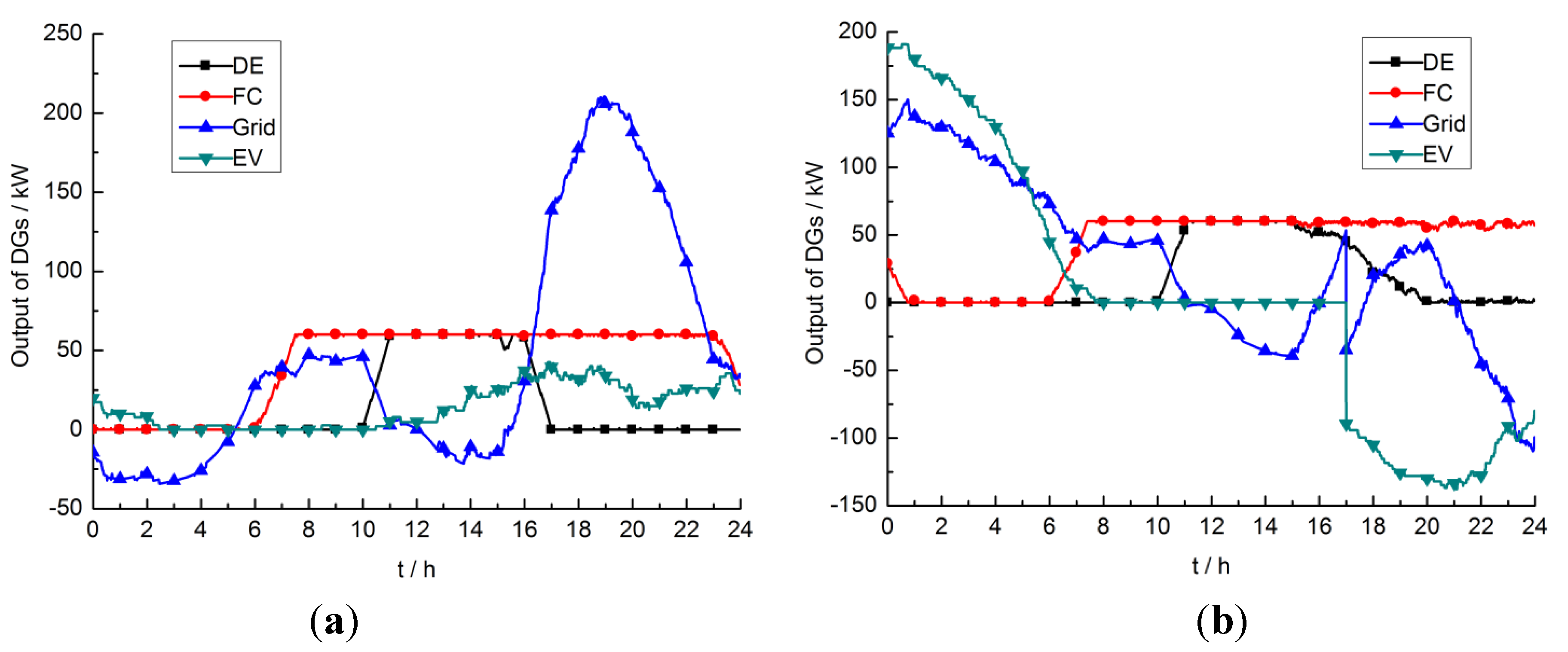
6.4.1. Analysis of the Output of DGs
After economic dispatch of the microgrid system, the scheduling results of EVs, FCs, DEs and the power grid are shown in
Figure 5. Due to the strategy to maximize the utilization of renewable energy, the figure does not show the wind and solar power profiles.
Figure 5.
(a) Dispatch results under scheduling strategy 1; (b) Dispatch results under scheduling strategy 2.
Figure 5.
(a) Dispatch results under scheduling strategy 1; (b) Dispatch results under scheduling strategy 2.
When the microgrid system adopts scheduling strategy 1, it can be seen from
Figure 5a that from 0:00 to 5:00, the power grid output is negative; that is, the microgrid feeds excess electricity to the power grid. This is because the WT output is larger than the load demand of the microgrid. After 5:00, the renewable energy output is unable to meet the load demand, so the power grid is used due its lower comprehensive objective cost. After 6:00, FC is enabled and has priority to be scheduled from that time according to the maximum output power due to its lower objective cost. After 10:00, the objective cost of the power grid becomes higher than DE, so DE replaces the power grid to output power. From 11:00 to 16:00, the costs of DE and FC are lower than the power grid, therefore the excess electricity is fed to the power grid to improve the economics after meeting the load demand. After 16:00, the cost of DE is higher than the power grid, so it is gradually replaced by the power grid.
When the microgrid system adopts scheduling strategy 2, it can be seen from
Figure 5b that the EV charging load is concentrated from 0:00 to 7:00. During that period, the comprehensive objective costs of the power grid and FC are lower than DE, so they output power together. After 6:00, FC has priority to be scheduled due to its lower objective cost. From 7:00 to 17:00, EVs are not involved in scheduling. In that period, before 10:00 the objective cost of the power grid is lower than DE, so it outputs power together with FC. From 10:00 to 16:00, the objective cost of DE is lower than the power grid, so instead of the power grid, it supplies power together with FC. In the meantime, if the objective costs of DE and FC are lower than the power grid, then the excess electricity is fed to the power grid to improve the economics after meeting the load demand. After 16:00, the objective cost of DE is higher than the power grid, so it stops being used. After 17:00, EVs begin to discharge, which means participating in scheduling, so the power grid output is reduced. After 21:00, EVs begin to feed power to the power grid, which can bring economic benefits to EV owners.
6.4.2. Analysis of the Objective Function Cost
The three objective functions cost and the comprehensive objective function cost of scheduling under scheduling strategy 1 and 2 are shown in
Table 6. Due to the randomness of the particle swarm optimization algorithm, the following table shows the average cost after repeatedly calculating 20 times.
Table 6.
Grid-connected mode: cost of dispatch results under different strategies.
Table 6.
Grid-connected mode: cost of dispatch results under different strategies.
| Cost/¥ | Scheduling strategy 1 | Scheduling strategy 2 | |
|---|
| C1 | 973.55 | 684.66 | −29.67% |
| C2 | 223.33 | 386.68 | 73.14% |
| C3 | 152.85 | 332.53 | 117.55% |
| C | 693.84 | 570.82 | −17.73% |
From the data in the
Table 6, it can be seen that adopting scheduling strategy 2 reduces by 17.73% the comprehensive objective cost compared with adopting scheduling strategy 1, which reduces by 29.67% the operating cost, increases by 73.14% pollutant emissions, and increases by 117.55% the carbon dioxide emissions. This result indicates that when the microgrid is running under the grid-connected mode, the EV coordinated charging and discharging mode can lower the operating cost, but carbon emissions and pollutant emissions are higher. This is because when the scheduling objective function is comprehensive, the weight coefficient of the operating cost is 0.6370, and the first, second and third level objectives cannot achieve their best in the meantime.
Contrasting
Figure 5a,b, the EVs are charging in the off-peak load periods at night to avoid the peak load, and discharging at peak load periods in order to achieve peak load shifting and reduce the cost of purchasing electricity from the power grid. Thus, adopting the EV coordinated charging and discharging mode is not only conducive to the stability of the microgrid system operation, but also reduces the operating cost.
6.5. Scheduling Results Analysis When the Microgrid Is Running under the Island Mode
6.5.1. Analysis of the Output of DGs
After economic dispatch of the microgrid system, the scheduling results of EVs, FCs, DEs and LS are shown in
Figure 6.
Figure 6.
(a) Dispatch results under scheduling strategy 3; (b) Dispatch results under scheduling strategy 4.
Figure 6.
(a) Dispatch results under scheduling strategy 3; (b) Dispatch results under scheduling strategy 4.
When the microgrid system adopts scheduling strategy 3, it can be seen from
Figure 6a that from 0:00 to 6:00, the total load of the microgrid is small, so the BS is charging during this period. After that time, DE and FC output power together. Around 11:00 to 12:00, DE and FC cannot meet the load demand even to output in the upper limit, and BS has not been put into use yet, and there appears a power shortfall, so it is necessary to cut off part of the interruptible load. From 16:00 to 22:00, there are more power shortfalls due to EV charging, and in the meantime, BS discharges to reduce both the peak load and the power shortfall. After that time, the microgrid load demand is decreased and renewable energy generations, DE, and FC output power are used together to meet the load demand and charge the BS.
When the microgrid system adopts scheduling strategy 4, it can be seen from
Figure 6b that the load of EV charging is concentrated from 0:00 to 7:00, resulting in a significant increase in the load demand. DE and FC output cannot meet the demand, so the BS is controlled to discharge. From 7:00 to 17:00, EVs are not involved in scheduling, and the system load is powered by DE and FC. From 16:00 to 17:00, DE and FC output cannot meet the load demand, and there appears a power shortfall, so part of the interruptible load is cut off. After 17:00, EVs begin discharging to participate in scheduling and charge the BS. After 20:00, because the comprehensive objective costs of DE and FC are higher than V2G, then their output is gradually reduced until they stop being used. In
Figure 6a,b, the area surrounded by the BS power profile under the zero axis and above is substantially equal, implying that the SOC at the beginning and end of a dispatch cycle remains the same.
6.5.2. Analysis of the Objective Function Cost
The three objective functions cost and comprehensive objective function cost of scheduling results under scheduling strategy 3 and 4 are shown in
Table 7. Due to the randomness of the particle swarm optimization algorithm, the following table shows the average cost after repeatedly calculating 20 times.
Table 7.
Island mode: cost of dispatch results under different strategies.
Table 7.
Island mode: cost of dispatch results under different strategies.
| Cost/¥ | Scheduling strategy 3 | Scheduling strategy 4 | |
|---|
| C1 | 1607.70 | 946.84 | −41.11% |
| C2 | 569.02 | 560.10 | −1.57% |
| C3 | 235.27 | 256.79 | 9.15% |
| C | 1195.72 | 786.16 | −34.25% |
From the data in the
Table 7 it can be seen that adopting scheduling strategy 4 reduces by 34.25% the comprehensive objective cost compared with adopting scheduling strategy 3, which reduces by 41.11% the operating cost, reduces by 1.57% pollutant emissions, and increases by 9.15% the carbon dioxide emissions. This indicates that when the microgrid is running under the island mode, the EV coordinated charging and discharging mode can lower the operating cost and pollutant emissions, but the carbon dioxide emissions are higher. Contrasting
Figure 6a,b, during the peak load periods, EVs charging increases the load peaks when adopting the EV autonomous charging mode, resulting in a significant compensation cost for LS. Meanwhile, the EVs discharging avoids a lot of LS when adopting the EV coordinated charging and discharging mode, thereby reducing the operating cost, but the charging is concentrated at night, increasing the DE and FC use time, so carbon dioxide emissions are higher. In summary, the adoption of the EV coordinated charging and discharging mode can reduce the power shortfall when the microgrid system is running under the island mode, and helps to improve the operation economics.
6.6. The Influence of Load Uncertainty
Research shows that the load fluctuation of the power system is generally described by a normal distribution [
24]. The probability density function is as follows:
where
δL is the standard deviation of load forecasting;
PL value of load forecasting;
PLf is value of actual load.
In the microgrid system economic dispatch process, in order to ensure the reliability of system operation, the uncertainty of load fluctuation can be stabilized by spinning reserve. In this paper, we study the impacts of load uncertainty on economic dispatch when the microgrid is running under the grid-connected mode, and the spinning reserve is powered by the power grid. The operating cost is the first level objective among the three objectives, reflecting the economic situation of the microgrid system, so we choose objective function 1 as the scheduling objective for economic dispatch in this section.
Table 8 shows the operating cost when the load fluctuation is 0%, 5%, 10%, 15% and 20%, respectively. Due to the randomness of the normal distribution function, the following table shows the average cost after repeatedly calculating 20 times.
Table 8.
Total cost of dispatch results under different load fluctuations.
Table 8.
Total cost of dispatch results under different load fluctuations.
| Scheduling strategy 1 | Scheduling strategy 2 | |
|---|
| C1/¥ | Increase | C1/¥ | Increase |
|---|
| 0% | 1035.42 | 0% | 675.98 | 0% | −34.71% |
| 5% | 1069.90 | 3.33% | 709.46 | 4.95% | −33.69% |
| 10% | 1101.51 | 6.39% | 757.27 | 12.03% | −31.25% |
| 15% | 1154.92 | 11.54% | 796.70 | 17.86% | −31.02% |
| 20% | 1207.57 | 16.63% | 839.13 | 24.14% | −30.51% |
Table 8 shows that if the load fluctuation increases, the microgrid operating cost will increase too, no matter whether scheduling strategy 1 or 2 is used. This is because the greater the load fluctuation, the more spinning reserve capacity the microgrid needs. So the purchasing electricity cost from the power grid is higher, and the operating cost is also higher.
In addition, under the same load fluctuation, the operating cost of the system when EVs are charging and discharging under the coordinated mode is lower than the cost when they are charging under the autonomous mode. In
Table 8, when the load uncertainty parameter increases from 0% to 5%, 10%, 15% and 20%, the operating cost is reduced by 34.71%, 33.69%, 31.25%, 31.02%, and 30.51%, respectively, which indicates that the coordinated charging and discharging mode of EVs has better operation economics.
7. Conclusions
According to the spatial and temporal characteristics of EVs, this paper established an autonomous charging model and coordinated charging and discharging model of EVs. Based on the current studies on multi-objective economic dispatch of the microgrid system, we determined the lowest operating cost, the lowest pollutant treatment cost and the least carbon dioxide emissions as objective functions. We then developed four different scheduling strategies under the grid-connected mode and the island mode of the microgrid operation. Next we established the model of multi-objective economic dispatch of the microgrid system including V2G. The judgment matrix method is used to convert the multi-objective functions to a single objective function. Considering the constraints of safety operation, the validity of the model and the algorithm is verified through simulation of an example system by using an improved particle swarm algorithm based on different scheduling strategies. The simulation results show that the EV coordinated charging and discharging mode has better operation economics than the autonomous charging mode. Meanwhile, the greater the load fluctuation is, the higher the operating cost of the microgrid system is.


