Using Satellite SAR to Characterize the Wind Flow around Offshore Wind Farms

Abstract

Offshore wind farm cluster effects between neighboring wind farms increase rapidly with the large-scale deployment of offshore wind turbines. The wind farm wakes observed from Synthetic Aperture Radar (SAR) are sometimes visible and atmospheric and wake models are here shown to convincingly reproduce the observed very long wind farm wakes. The present study mainly focuses on wind farm wake climatology based on Envisat ASAR. The available SAR data archive covering the large offshore wind farms at Horns Rev has been used for geo-located wind farm wake studies. However, the results are difficult to interpret due to mainly three issues: the limited number of samples per wind directional sector, the coastal wind speed gradient, and oceanic bathymetry effects in the SAR retrievals. A new methodology is developed and presented. This method overcomes effectively the first issue and in most cases, but not always, the second. In the new method all wind field maps are rotated such that the wind is always coming from the same relative direction. By applying the new method to the SAR wind maps, mesoscale and microscale model wake aggregated wind-fields results are compared. The SAR-based findings strongly support the model results at Horns Rev 1.

1. Introduction

In the Northern European Seas offshore wind farms are planned as clusters. The wind farm wake from one wind farm thus has the potential to influence the power production at neighboring wind farms. The expected wake loss due to wind farm cluster effects is investigated in the present study. The wind farm wake cluster effects are strongly dependent upon the atmospheric conditions. These vary spatially and temporally. One remote sensing method for observing ocean surface winds is satellite Synthetic Aperture Radar (SAR). The advantage of SAR is that a large area is observed and several wind farms are covered. The derived wind map from SAR provides a snapshot of the wind field during a few seconds at the time of acquisition.

In the satellite SAR data archives covering the North Sea, thousands of wind turbines are visible as white dots in calm conditions. For low wind speed the backscatter signal over the ocean is low and the images appear dark while hard targets such as wind turbines and ships provide high backscatter and the objects appear very bright. During windy conditions wind farm wakes are sometimes visible as dark elongated areas downwind of a wind farm while the surrounding seas appear brighter. This is a result of the differences in wind speed with reduced winds downwind of large operating wind farms. The intensity of backscatter of microwave electromagnetic radiation from the ocean surface is a non-linear function of the wind speed over the ocean. The physical relationship is due to the capillary and short gravity waves formed at the ocean surface by the wind. For higher wind speeds the backscatter is higher.

Previous wind farm wake studies based on SAR from ERS-1/-2, Envisat, RADARSAT-1/-2, TerraSAR-X and airborne SAR show great variability in wind farm wakes [1,2,3,4]. This reflects the natural variability in atmospheric conditions at the micro- and mesoscale. Wind farm wakes are often not clearly visible in the SAR archive data. This may be explained by wind turbines out of operation or presence of oceanic features, e.g., bathymetry, currents, surfactants. However, the great variability in the wind field is most likely a major cause.

In order to show that wind farm wakes are detectable from SAR, we present in this study one case based on RADARSAT-2 ScanSAR Wide. This scene is a good example where ideal conditions for wake analysis occur and the coverage is just right for capturing 10 large offshore wind farms located in the southern North Sea. We compare the instantaneous SAR-based wind farm wakes to micro- and mesoscale wake model results.

For the rest of our SAR wind archive, we wish to find out if wakes can be detected even if they are not so clearly visible. We first use a simple method which has some disadvantages. Next we apply the aggregated method to overcome some of these disadvantages.

This is the first time that a suitable number of SAR scenes covering several large operating winds farms have become available [5]. The present study focuses on the wind farm wake climatology using many overlapping SAR scenes. The wide-swath-mode (WSM) products from the Advanced SAR (ASAR) on-board Envisat are selected. This data source is sampled routinely so there are many more samples but with less spatial detail (original resolution 150 m) than those used in previous studies (of the order 5 to 30 m spatial resolution) where the data are rare and infrequent and only sampled upon request [1,2,3,4]. It is questionable whether wake effects can be detected from Envisat ASAR WSM data as we cannot always visually see the wind farm wakes. However, we hypothesize that the combination of many satellite samples will show an aggregated effect of the wind farm wakes on the mean wind climate in the area. The SAR-based wind farm wake climatology results therefore can be used to validate wake model results. The wind farm wake climatology can be modelled by micro- and mesoscale models but perfect agreement cannot be expected between SAR and wake model results. This is due to the different nature of data with SAR based on the sea surface while wake models operate around wind turbine hub-height.

The main topic of the study is on the potential of using SAR for characterization of wind flow around offshore wind farms. Our mission is to find out how to best utilize SAR for wake mapping. Three modes of investigation are considered: (1) Wind flow observed at 10 offshore farms with wind farm wakes concurrent in one SAR scene; (2) Wind flow observed at two wind farms concurrent and wind farm wakes average value based on 7 to 30 SAR scenes; (3) Wind flow observed at one wind farm at a time and the aggregated wind farm wake based on 100 to 800 SAR scenes. Basic information on the three modes of investigation is listed in Table 1. The advantages and limitations of each investigation mode in regard to wind farm wake model comparison are provided. Selected wake model results are presented as demonstration for each of the modes. Presenting the three modes in such an order clearly shows the evolution of wake studies using SAR.

Table 1. SAR source, number of wind farms covered in the method, number of SAR scenes used in each method for wake identification based on no averaging, geo-located SAR wind field averaging and rotated SAR wind field averaging. The spatial resolution of the wind fields are given. The Section in this paper where each mode is presented is also indicated.

Satellite Data	Number of Wind Farms	Number of SAR Scenes	Averaging	Analysis Type	Resolution (km)	Section
RADARSAT-2	10	1	None	Qualitative	1	3
Envisat ASAR	2	7–30	Geo-located	Quantitative	1	4
Envisat ASAR	1	100–800	Rotated	Quantitative	1	5

Table 1. SAR source, number of wind farms covered in the method, number of SAR scenes used in each method for wake identification based on no averaging, geo-located SAR wind field averaging and rotated SAR wind field averaging. The spatial resolution of the wind fields are given. The Section in this paper where each mode is presented is also indicated.

Satellite Data	Number of Wind Farms	Number of SAR Scenes	Averaging	Analysis Type	Resolution (km)	Section
RADARSAT-2	10	1	None	Qualitative	1	3
Envisat ASAR	2	7–30	Geo-located	Quantitative	1	4
Envisat ASAR	1	100–800	Rotated	Quantitative	1	5

The structure of the paper includes in Section 2 a description of the study site, satellite data and the two wake models used. In Section 3 the results from the case study based on RADARSAT-2 and the results from two wake models are presented and discussed. Section 4 presents the Envisat SAR-based wind farm wake climatology based on simple averaging of the wind fields at Horns Rev 1 and 2 wind farms and comparison to results from one wake model. Section 5 gives introduction to the new methodology developed in which the wind field maps are rotated such that the wind is always coming from the same relative direction. The Envisat SAR-based results from the new methodology as well as wake model results from two models are presented and Envisat SAR-based results from four other wind farms are presented. In Section 6 is the discussion of results. Conclusions are given in Section 7.

2. Study Site, Satellite SAR and Wake Modelling

2.1. Study Site

Wind flow around the wind farms in the southern part of the North Sea is investigated. The wind farms studied are listed in Table 2 and the location of most of the wind farms is shown in Figure 1. Those not shown in Figure 1 are the Alpha ventus wind farm located in the German North Sea and Horns Rev 1 and 2 located in the Danish North Sea. The information in Table 2 includes the year of start of operation and key data on the wind turbines and area covered.

Figure 1. RADARSAT-2 intensity map of the southern North Sea observed 30 April 2013 at 17:41 UTC. The blue lines outline wind farms and the red arrows the wind farm wake.

Figure 1. RADARSAT-2 intensity map of the southern North Sea observed 30 April 2013 at 17:41 UTC. The blue lines outline wind farms and the red arrows the wind farm wake.

Table 2. Wind farm info: Country, start year of operation, approximated latitude and longitude, number and size of turbines, wind park capacity and area covered.

Wind Farm	Nationality	Year	Latitude (°)	Longitude (°)	Number of Turbines	Turbine Size (MW)	Park (MW)	Area (km2)
Alpha ventus	Germany	2009	54.010	6.606	12	5	60	4
Belwind 1	Belgium	2010	51.670	2.802	55	3	165	13
Greater Gabbard	United Kingdom	2012	51.883	1.935	140	3.6	504	146
Gunfleet Sands 1 + 2I	United Kingdom	2010	51.730	1.229	48	3.6	172.8	16
Horns Rev 1	Denmark	2002	55.486	7.840	80	2.0	160	21
Horns Rev 2	Denmark	2009	55.600	7.582	91	2.3	209.3	33
Kentish Flats	United Kingdom	2005	51.460	1.093	30	3	90	10
London Array Phase 1	United Kingdom	2012	51.626	1.495	175	3.6	630	100
Thanet	United Kingdom	2010	51.430	1.633	100	3	300	35
Thornton Bank 1	Belgium	2009	51.544	2.938	6	6	30	1
Thornton Bank 2	Belgium	2012	51.556	2.969	30	6.15	184.5	12
Thornton Bank 3	Belgium	2013	51.540	2.921	18	6.15	110.7	7

Table 2. Wind farm info: Country, start year of operation, approximated latitude and longitude, number and size of turbines, wind park capacity and area covered.

Wind Farm	Nationality	Year	Latitude (°)	Longitude (°)	Number of Turbines	Turbine Size (MW)	Park (MW)	Area (km2)
Alpha ventus	Germany	2009	54.010	6.606	12	5	60	4
Belwind 1	Belgium	2010	51.670	2.802	55	3	165	13
Greater Gabbard	United Kingdom	2012	51.883	1.935	140	3.6	504	146
Gunfleet Sands 1 + 2I	United Kingdom	2010	51.730	1.229	48	3.6	172.8	16
Horns Rev 1	Denmark	2002	55.486	7.840	80	2.0	160	21
Horns Rev 2	Denmark	2009	55.600	7.582	91	2.3	209.3	33
Kentish Flats	United Kingdom	2005	51.460	1.093	30	3	90	10
London Array Phase 1	United Kingdom	2012	51.626	1.495	175	3.6	630	100
Thanet	United Kingdom	2010	51.430	1.633	100	3	300	35
Thornton Bank 1	Belgium	2009	51.544	2.938	6	6	30	1
Thornton Bank 2	Belgium	2012	51.556	2.969	30	6.15	184.5	12
Thornton Bank 3	Belgium	2013	51.540	2.921	18	6.15	110.7	7

2.2. Satellite SAR

SAR data from RADARSAT-2 and Envisat ASAR WSM are used. From RADARSAT-2 only one scene is investigated. It is ScanSAR Wide in VV polarization. The wind field retrieval requires input information about the wind direction. From the RADARSAT-2 image the wake direction has been estimated as 40° and using this input for wind direction, wind speed has been retrieved using CMOD-IFR2 [6]. It is the equivalent neutral wind (ENW) at the height 10 m. The calculated wind speed is presented in Figure 2a. The original ScanSAR Wide product has spatial resolution 100 m. The spatial resolution is reduced to approx. 1 km in connection with the processing of wind fields. This is performed to eliminate effects of random noise and long-period waves.

Figure 2. (a) Satellite 10-m SAR wind retrieval observed 30 April 2013 at 17:41 UTC and (b) modified PARK wake results at 70 m for the wind farms in the UK and Belgium. The wind direction used for the modeling is indicated with the black arrow.

Figure 2. (a) Satellite 10-m SAR wind retrieval observed 30 April 2013 at 17:41 UTC and (b) modified PARK wake results at 70 m for the wind farms in the UK and Belgium. The wind direction used for the modeling is indicated with the black arrow.

The Envisat ASAR data were processed to wind fields as part of the project NORSEWInD [5]. The wind field retrieval gives the ENW at the height 10 m. For processing of large image archives, it is desirable to use wind direction information from an atmospheric model. In this case the wind directions were obtained from the European Centre for Medium-Range Weather Forecasts (ECMWF) model and interpolated spatially to match the higher resolution of the satellite data. Further details about the SAR-wind processing chain, which was setup by Collecte Localisation Satellites (CLS), are given in [5]. The original WSM product has spatial resolution 150 m. The spatial resolution is to approx. 1 km in the wind field.

2.3. Wake Modelling with PARK and WRF

A modified version of the PARK wake model [7], also implemented in the Wind Atlas Analysis and Application Program (WAsP) [8], is here used for wake calculations. The main difference between this modified version and that in WAsP is that the former does not take into account the effects of the “ground reflecting back wakes” and so it only takes into account the shading rotors both directly upstream and sideways. The PARK wake model is based on the wake deficit suggested by [9], who derived a mass-conservation-like equation for the velocity immediately before a turbine u₂, which is affected by a wake:

$$u_2=u_1\left[1-\frac{a}{{\left(1+\frac{k_{\text{w}}x}{r_{\text{r}}}\right)}^2}\right]$$

(1)

where u₁ is the upstream wind speed, a the induction factor which is a function of the thrust coefficient (C_t), k_w the wake decay coefficient, x the downstream distance and r_r the turbine’s rotor radius. The square of the total wake deficit is estimated as the sum of the square of all contributing wake deficits. We implemented the model in a Matlab script. This allows us to compute wake deficits at any given point. The wake model can be compared to satellite derived wind maps which contains information over a large area. We use k_w = 0.03 for the wake computations.

The Weather Research and Forecasting (WRF) mesoscale model [10] is also used for wake modelling. The advantage of WRF is that the dynamic synoptic flow is considered. The computational cost is much higher than that for the PARK model though.

Mesoscale models have been developed to simulate the atmosphere flow over areas on the order of hundreds of kilometers. Due to their low horizontal resolution unresolved processes, such as turbulence and turbine induced wakes have to be parametrized. In common wind farm parametrisations [11,12,13,14,15,16] the local turbine interaction is not accounted for, instead the wind speed reduction within the wind farm is obtained from the interaction between the turbine containing grid-cells. The Explicit Wake Parametrisation (EWP) is used for the parametrization of wind farms [16]. In this approach a grid-cell averaged deceleration is applied, which accounts for the unresolved wake expansion with the turbine containing grid-cell. Turbulence Kinetic Energy (TKE) is provided by the Planetary Boundary Layer (PBL) scheme from a changed vertical shear in horizontal velocity in the wake. The EWP scheme is independent of the PBL scheme, although, a second order scheme is recommended.

We use WRF V3.4 with the selected mesoscale model physics parametrizations: PBL [17] (MYNN 2.5), convection [18] (Domain I and II), micro-physics [19], long-wave radiation [20], shortwave radiation [21], land-surface [22] and Nudging of U and V in the outer domain (outside PBL). The number of grid cells in the innermost domain were 427 times 304 in the x and y direction, with a 2 km grid-spacing. We used [16] for the wind farm parametrization.

The model outer domain is driven by ERA-Interim reanalysis data [23] and two nests are inside. The horizontal resolution for the three domains is 18 km, 6 km and 2 km, respectively. The inner nest is run twice, without and with the wind farm parametrization. The number of vertical layers is set to 60. The second mass level is at around 12 m above sea level and it is used for the comparison to the satellite images.

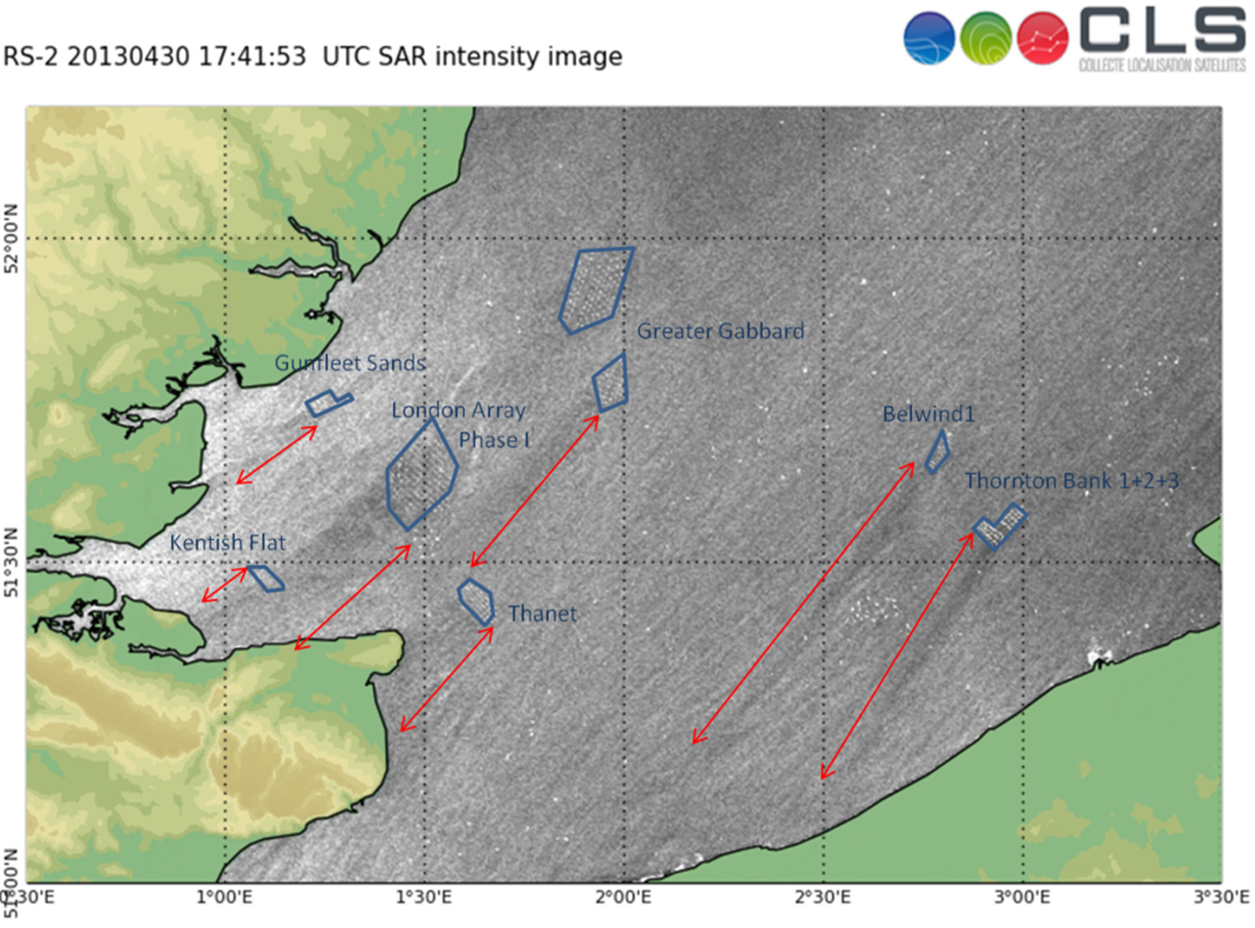
3. Case Study Based on RADARSAT-2

The case study is based on the RADARSAT-2 scene from 30th April 2013 at 17:41 UTC (selected from around 30 images with visible wakes). Figure 1 shows the backscatter intensity map. The wind is from the northeast and the map shows elongated long dark areas downwind of most of the wind farms. These are the wind farm wakes. The approximate extent of the individual wind farm wakes is outlined in the image. The longest is at Belwind around 55 km long while at Thornton Bank it is 45 km, London Array 15 km and Thanet 14 km. At Kentish Flat the wind farm wake is only 10 km long but it is probably passing over the coast and inland in the UK. This cannot be mapped from SAR. It should be noticed that all wakes are very straight and with similar direction. In the intensity map the wind turbines can be seen as small regularly spaced white dots while numerous ships can be noted in irregular spatial pattern. Some large ships show higher backscatter than the turbines.

The retrieved wind speed map is shown in Figure 2a. The wind speed in the northern part of the map is slightly lower than in the southern part. Yet the synoptic flow appears to be fairly homogenous across the entire area. Coastal speed up is seen particular near the UK and Belgium coastlines. The wind speed varies around 8.5–9.5 m·s⁻¹ in areas not affected by wind farms while the wind farm wake regions show lower wind speed around 7–8 m·s⁻¹ dependent upon location. The wake at London Array is very wide and it appears to influence Kentish Flat at this time. The wake at London Array has a large wake deficit with much lower wind speeds in the wake than in the upwind free stream region. Wake meandering is not pronounced.

The case illustrates a rather unique situation. Firstly because we observe wakes in the satellite image for all wind farms distributed in a large area of the North Sea (all farms in the area show clear speed deficits). Secondly the wind speed and wind the direction do not seem to largely change over such an extended area. Therefore we are able to simulate with the PARK wake model all wind farms at the same time (assuming the same background inflow conditions for all of them). The background wind speed is about 9 m·s⁻¹ and direction 40°. We use these two values at 70 m as inflow conditions for the wake modeling.

Figure 2a shows the SAR wind retrieval at 10 m, where most of the variability seems to come from the wake deficits downstream the wind farms, and the wake model results at 70 m in Figure 2b. In this case, we do not extrapolate the satellite background conditions up to 70 m or extrapolate downwards the model results to 10 m as we assume the same wind speed at around hub height when performing the wake simulations. The comparison is only qualitative.

Interestingly, the speed deficits seem to be rather well reproduced by the wake model, extending in most cases nearly as long as the wakes observed in the SAR image.

The WRF wake model with the EWP wind farm scheme is also used for simulation. We include only London Array, Greater Gabbard, Thanet, Belwind1 and Thornton Bank which are the largest wind farms. The domain is rotated around 10° at the wind farm location. The simulation is from the 24 April to 1 May 2013. The velocity deficit at 10 m at 30 April 2013 at 18:00 UTC is shown in Figure 3. We have chosen to plot the velocity deficit since due to the gradients in the background velocity the wake is not visible in the velocity field from the wind farm simulation.

Figure 3. WRF wake model results on velocity deficit in m·s⁻¹ at 10 m AMSL at 30 April 2013 at 18:00 UTC at the wind farms London Array, Greater Gabbard, Thanet, Belwind 1 and Thornton Bank.

Figure 3. WRF wake model results on velocity deficit in m·s⁻¹ at 10 m AMSL at 30 April 2013 at 18:00 UTC at the wind farms London Array, Greater Gabbard, Thanet, Belwind 1 and Thornton Bank.

The WRF modelled wakes at the UK wind farms are oriented slightly more towards the eastern direction than the satellite wakes. The orientations differ by around 10°. For the Belgian wind farms we find that the wakes are well aligned in the SAR and WRF results. Regarding the wake extension behind the wind farms we find for the London Array short wakes both in SAR and WRF while the wakes at the Thanet and Greater Gabbard wind farms are considerably longer both in SAR and WRF. However WRF shows even longer wakes than SAR for Greater Gabbard and Thanet. The extension of wakes at the Belgian wind farms compare well in SAR and WRF.

From WRF it is found that the synoptic conditions two hours before 18:00 UTC show intensified pressure gradients, leading to increased wind speeds near the English coast from 4 m·s⁻¹ to higher winds in the order of 10 m·s⁻¹. The Greater Gabbard and Thanet wind farms experienced high wind speeds for two hours at 18:00 UTC. The wind speeds started to increase at the London Array only shortly before 18:00 UTC. It might be that the increasing model wind speeds are for some hours out of phase, which would explain the longer wakes behind Greater Gabbard and Thanet wind farms in WRF compared to SAR.

In summary, the wind farm wakes from several wind farms are visually compared between SAR and WRF simulations of the velocity deficit obtained without wind farm and with wind farms using the EWP scheme. The wind farm wake directions and extension of wake are found to compare well despite that mesoscale features, such as that resulting from unsteady flow conditions, are noted in the wind farm wakes in the WRF simulation. We cannot expect the WRF simulations to match the observed velocity and wind direction in SAR satellite data perfectly. The PARK model results do not include unsteady flow but even so the PARK model results have overall good agreement to SAR. This can in part be attributed to the rather unique atmospheric conditions at the time of this SAR acquisition. The results for single events only can be used qualitatively. For a quantitative comparison statistics over longer periods are needed.

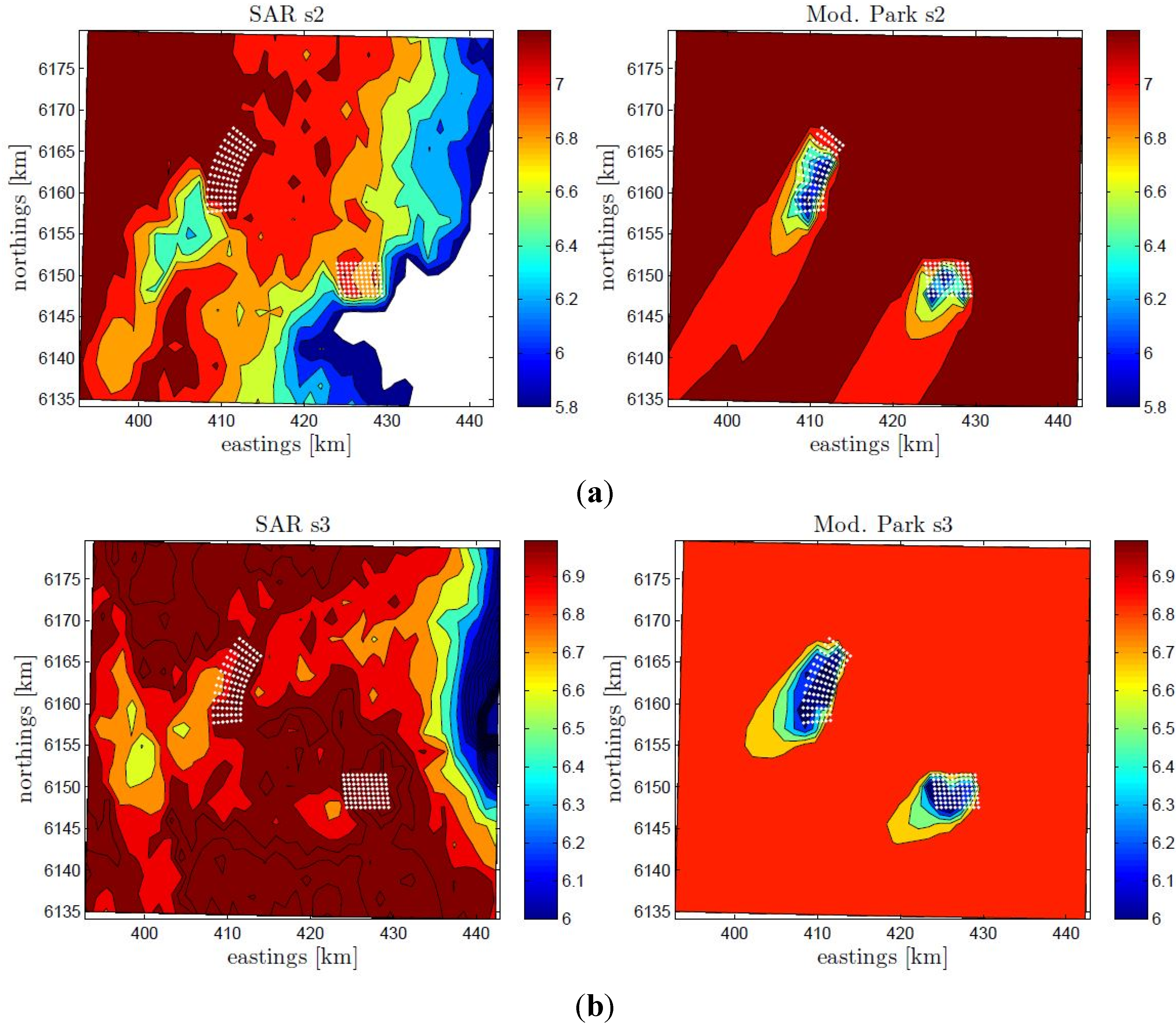
4. Wind Farm Wake Climatology Geo-Located Wind Maps

The case in Section 3 was selected based on clear visual observation of wind farm wakes at several wind farms within one satellite SAR image. However, we would like to study the behavior of the wind farm wake in a climatological fashion and investigate whether this can be performed using our Envisat ASAR WSM data set. We select to study the Horns Rev 1 and 2 wind farms for which we have 356 SAR scenes in total for the period of dual wind farm operation from September 2009 to the termination of the Envisat mission in March 2012.

As the wake behavior is highly dependent on the inflow wind conditions, in particular the wind direction, we perform the study for 12 directional sectors based on the ECMWF model wind direction used to retrieve the SAR winds. The SAR scenes are first binned according to the wind directions extracted for a single point near the two wind farms. The data set is then filtered such that only scenes with wind speeds in the range 4–14 m·s⁻¹at the same point are included (total of 241). This is the range where wind farm wakes are expected to be most detectable. At lower wind speeds, the turbines are not operating and at higher wind speeds, wind penetration through the wind farms is expected. For each directional bin, we extract the inflow conditions from a point upstream of the wind farms for every SAR scene in the bin. The reference points are located on two circles circumscribing the wind farms Horns Rev 1 and Horns Rev 2 with radii of 7.5 km and 10 km, respectively, as shown in Figure 4. To get representative inflow conditions, the satellite winds are extracted within a radius of 10 km for Horns Rev 2 and a radius of 7.5 km for Horns Rev 1 wind farm.

Figure 4. Horns Rev 1 and 2 wind farms in red and black markers, respectively. The locations of the points where the inflow conditions are extracted per sector (cyan markers) is also illustrated.

Figure 4. Horns Rev 1 and 2 wind farms in red and black markers, respectively. The locations of the points where the inflow conditions are extracted per sector (cyan markers) is also illustrated.

We perform simulations using the modified PARK model at all positions on the satellite grid and for all the inflow conditions per sector. The point around the wind farms where we extract the inflow conditions is selected based on the sector analyzed, e.g., we use the point north of Horns Rev 2 when performing simulations for Sector 1. In the following subsections we perform qualitative comparisons of the 10 m wind speed SAR retrievals with the results of the wake model per sector at the same height. Both results (wind speed maps) show the average wind speed per sector. We choose to show results for Sector 2 and 3 in Figure 5 because the coastal wind speed gradient and wind farm wakes can be seen in these results even though relatively few data are available. Table 3 shows the number of samples per sector. The inflow wind speed for Sector 2 and Sector 3 is 8.52 and 8.25 m·s⁻¹ in average with a standard deviation of 3.50 and 2.55 m·s⁻¹, respectively (these are the values at 70 m height). This means that simulations are performed for a rather wide range of wind speeds. These two examples have several overlapping images and several features can be noted such as the coastal wind speed gradient and wind farm wake.

Figure 5. Average wind speed based on satellite SAR (left) and modified PARK wake model results (right) at 10 m height for the Horns Rev wind farm area for winds from Sector 2 (a) and Sector 3 (b). The color bar indicates wind speed in m·s⁻¹.

Figure 5. Average wind speed based on satellite SAR (left) and modified PARK wake model results (right) at 10 m height for the Horns Rev wind farm area for winds from Sector 2 (a) and Sector 3 (b). The color bar indicates wind speed in m·s⁻¹.

Table 3. Number of Envisat ASAR samples available per wind directional bin at Horns Rev.

Sector	1	2	3	4	5	6	7	8	9	10	11	12	Total
Samples	13	7	12	16	24	21	22	28	22	30	20	26	241

Table 3. Number of Envisat ASAR samples available per wind directional bin at Horns Rev.

Sector	1	2	3	4	5	6	7	8	9	10	11	12	Total
Samples	13	7	12	16	24	21	22	28	22	30	20	26	241

For Sector 2 there are seven available SAR images for the analysis and the average wind speed is 7.2 m·s⁻¹. It is surprising we do not observe wakes from the Horns Rev 1 wind farm (Figure 5a). This might be simply because of the high horizontal wind speed gradient approaching the coast, which is located east of Horns Rev 1. There is a clear wake spreading towards the southwest direction of the Horns Rev 2 wind farm. The PARK model results show clear wakes spreading southwest of both wind farms.

For Sector 3 twelve SAR images are available for the analysis (west of Horns Rev 2 the number is reduced to 10) with an average wind speed of 7.0 m·s⁻¹. This case shows agreement in terms of the location of the areas where wakes are observed in both the SAR and the PARK wake model at both wind farms (Figure 5b).

The number of samples per sector varies from 7 to 30 within the 12 sectors. The overall agreement between SAR and the wake model is variable. For some sectors (1 and 7) the bathymetry effect at Horns Rev appears to be particularly strong as previously noted by [1]. This results in the lack of wake effects in the mean wind speed maps from SAR due to the interaction of bathymetry and currents, which sometimes leaves a detectable “imprint” at the sea surface. This effect is most visible when winds blow directly from the north or south at Horns Rev (not shown here).

Another reason for the difficulties to systematically observe wakes of offshore wind farms from satellite-derived wind products are inhomogeneous flow. Although the ocean surface is rather homogenous, e.g., when compared to the land surface, the effects of the horizontal wind variability diminish those of the wakes. In the particular case of the Horns Rev area, there is a systematic wind speed gradient near the coast also obstructing the observation of wakes, particularly for easterly and westerly winds. These effects are not taken into account in the PARK modeling. The coastal gradient in wind speed is noticeable in the SAR images in Figure 5.

Finally it can be noted that the distribution of wind maps into direction sectors is performed with some uncertainty. The model wind directions used to drive the SAR wind speed retrieval are not always accurate. The accuracy of the wind direction input could be improved through implementation of higher-resolution regional model simulations, e.g., from WRF. Another option is to detect the wind direction directly from wake signatures whenever they are visible in the images. The distribution of satellite scenes into the 12 sectors is based on information extracted at a single point. Local turning of the wind is possible but not accounted for in the analysis. Each directional bin is 30° wide thus the peak wake directions are expected to vary within this and it will diffuse the observed aggregated wake features. Due to the nature of the SAR images (specifically its number) and due to other phenomena causing spatial variability in the wind speed (like coastal gradients and mesoscale phenomena), it seems not suitable to perform the SAR wake analysis per sectors this wide.

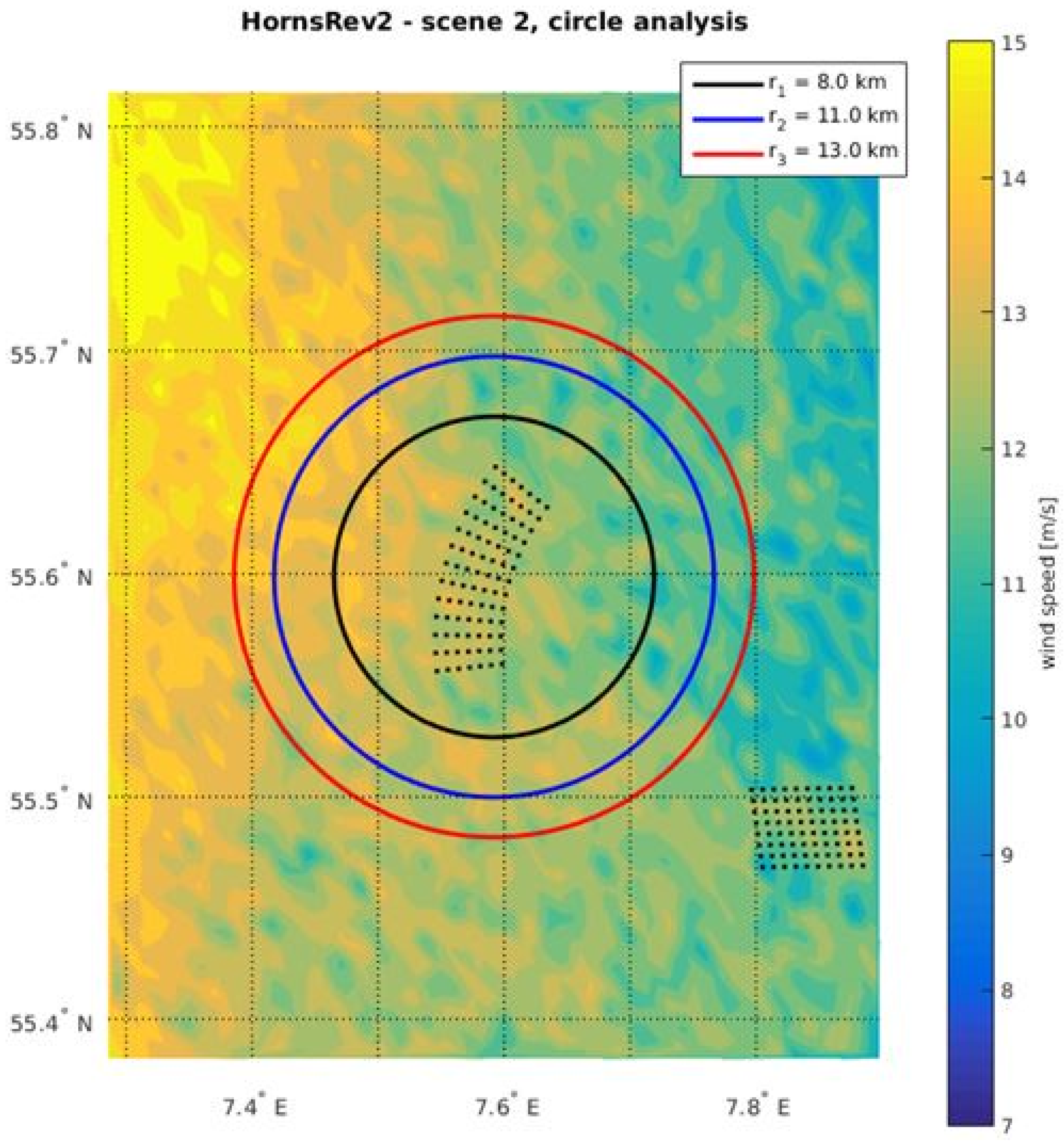
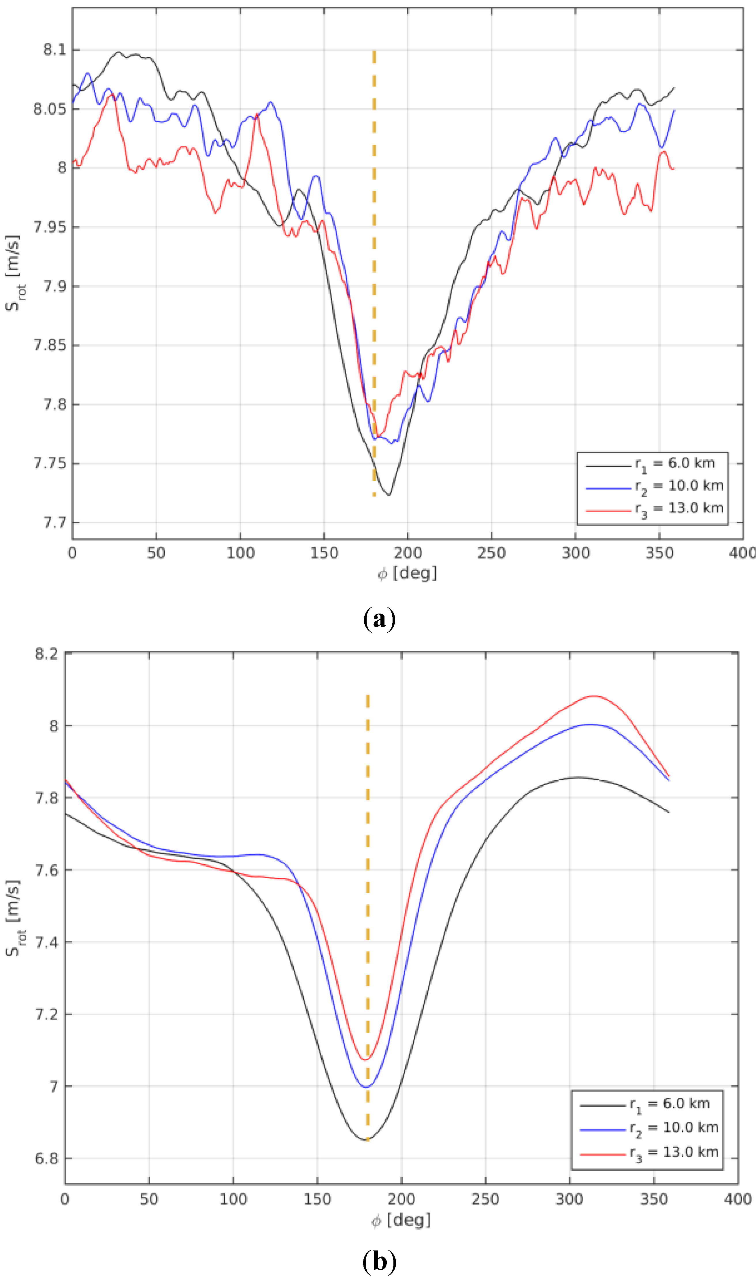
5. Wind Farm Wake Climatology Based on Rotation of Wind Maps

In this section a new approach to analyze SAR-derived wind farm wakes in a climatological way is presented. The method aligns (rotates) all SAR wind field samples such that the wind farm wakes are overlapping before the wake deficit is calculated. This increases the number of samples considerably compared to the method presented in Section 3. Furthermore the 30° wind direction bins used previously give diffuse results whereas in the new method wind directions alignment at 1° resolution is used. The new method is based on extracting wind speeds along points inscribed by circles centered on the wind farm under analysis. While the method was developed for analysis of wakes in SAR scenes, here it is also applied to the WRF simulations as a way to validate the mesoscale simulated wakes.

5.1. Description of the Method

For each SAR scene (or WRF simulated wind field) the wind speeds as a function of compass direction θ are extracted along 3 concentric circles centered on the wind farm. The radii depend on the wind farm in question, and are given in Table 3.

Figure 6 gives an example of the circles centered on the Horns Rev 2 wind farm. The wind fieldsare based on SAR data (1 km). It can be difficult to determine a wake by eye. For each SAR scene the wind speeds along these 3 circles are extracted and stored as U_i (θ_j), where U_i is the wind speed for circle i where i = 1, 2, 3 and θ_j is the compass direction relative to the center of the wind farm. θ_j steps through values from 0 to 359° with a 1 degree increment. The number of scenes used for the analysis depends on the wind farm under examination. The number is given in Table 4. The WRF model is run for all SAR scenes from Horns Rev 1 and 2, and results are extracted in a similar way from the WRF simulation results as for the SAR wind fields. The SAR results are valid at 10 m AMSL while WRF model results are available at 14 m AMSL.

Figure 6. Example of the circles centered on Horn Rev 2 wind farm. The radii are 8, 11 and 3 km.

Figure 6. Example of the circles centered on Horn Rev 2 wind farm. The radii are 8, 11 and 3 km.

Table 4. The radii of the three concentric circles for the different wind farms and the number of Envisat ASAR scenes used for the analysis.

Wind Farm	r1 (km)	r2 (km)	r3 (km)	Nscenes
Alpha ventus	5	10	15	245
Belwind1	6	11	15	97
Gunfleet Sands 1 + 2	4	5	6	153
Horns Rev 1	6	10	13	835
Horns Rev 2	8	12	15	303
Thanet	7	9	11	128

Table 4. The radii of the three concentric circles for the different wind farms and the number of Envisat ASAR scenes used for the analysis.

Wind Farm	r1 (km)	r2 (km)	r3 (km)	Nscenes
Alpha ventus	5	10	15	245
Belwind1	6	11	15	97
Gunfleet Sands 1 + 2	4	5	6	153
Horns Rev 1	6	10	13	835
Horns Rev 2	8	12	15	303
Thanet	7	9	11	128

First the sum of wind speeds is calculated:

$$S_i^N\left({\text{θ}}_j\right)=\frac{1}{N_{scene}}{\displaystyle \sum }_{k=1}^{N_{\text{scene}}}{(U_i({\text{θ}}_j))}_{k }$$

(2)

where k is the scene number, and N_scene is the total number of scenes. Figure 7a shows S^N plotted against θ, for the Horns Rev 1 wind farm. We see from this plot how the mean wind speed depends on θ. This can be explained in terms of the gradient of the mean wind in the vicinity of the coastline. We call this the coastal gradient. Similar results of S^N based on WRF are shown in Figure 7b. The coastal gradient in wind speed at Horns Rev 1 shows lowest values around 80°–110° (east), where the inscribed circles are closest to the coastline, and highest around 250° (west), where the inscribed circles are furthest from the coastline both in SAR and WRF. SAR shows a direction closer to 80° while WRF shows a direction closer to 110°. It is expected that there is an east-west gradient at Horns Rev as reported in [24]. For the eastern sector SAR shows higher wind speed values at the inner radius (6 km) and progressively lower values at outer radii (10 and 13 km) (nearer to the coastline). For the western sector SAR shows slightly higher wind speed at outer radii (further from the coastline).

WRF shows a similar pattern as SAR for the western sector but shows a reverse order in the wind speed at the eastern sector at different radii. This most likely is due to the simulated wake effects of Horns Rev 2 influencing the results at the 13 km radius around 260°–350°. This is supported by examining the results from using WRF without simulating the wind farms, shown in Figure 8. In this plot a very much cleaner signature of the coastal gradient is seen. The next step is to rotate the direction frame of reference for each SAR scene by using each scene’s reported wind direction, θ_k, to give a new direction reference, φ. In the new direction reference frame for each scene φ = 0° is aligned in the upwind direction and thus one may expect that the wake direction is in the region of φ = 180°. Now we can determine the wind speeds on the inscribed circles as a function of φ_j instead of θ_j by using:

$${\text{φ}}_j={\text{θ}}_j-{\text{θ}}_k$$

(3)

The sum of wind speeds for all scenes is now calculated with respect to the new direction frame, i.e.:

$$S_i^R({\text{φ}}_j)=\frac{1}{N_{\text{scene}}}{\displaystyle \sum }_{k=1}^{N_{\text{scene}}}{(U_i({\text{φ}}_j))}_k$$

(4)

Figure 7. Horns Rev 1 wind speed summations without rotation (mean wind speed gradient) (S) based on SAR (a) and WRF (b).

Figure 7. Horns Rev 1 wind speed summations without rotation (mean wind speed gradient) (S) based on SAR (a) and WRF (b).

Figure 8. Horns Rev 1 wind speed summations without rotation (S) based on WRF without wind farms, so showing only the coastal wind speed gradient.

Figure 8. Horns Rev 1 wind speed summations without rotation (S) based on WRF without wind farms, so showing only the coastal wind speed gradient.

Figure 9a shows S^R plotted against φ, for the Horns Rev 1 wind farm. The corresponding results of S^R based on WRF simulations are shown in Figure 9b. Please note that the differences between the top and bottom panels are due to the individual rotation of each scene prior to averaging and not the result of a single rotation by one angle. The similarity in form between SAR and WRF for the rotated maps (S_rot) is very good with low wind speeds showing at all radii at around φ = 180°. The inner radius shows more wake effect than outer radii. The SAR derived results are less smooth than those from WRF because the SAR scenes capture variability at smaller scales, due to the heterogeneity of the wind field, than is modelled by WRF.

To further reveal the wind farm wake from the heterogeneous wind field around the wind farm a method to calculate a wake wind speed deficit is employed. It is based on calculating a local perturbation of the wind speed on each SAR scene based on the side lobe wind speeds. The side lobe wind speeds are used at the directions φ + Δφ_i and φ − Δφ_i. For the smallest radius Δφ₁ = 90°, this means that the side lobe wind speed is from the left and right of the wind farm, at a distance of r₁ from the farm center. For the other radii, the side lobes have the same distance, r₁, from the line aligned with the wind direction and passing through the center of the wind farm, thus:

$$\mathrm{\Delta }{\text{φ}}_i=\text{arcsin}\left(\frac{r_1}{r_i}\right)$$

(5)

The wake wind speed deficit is defined by:

$$U_i^D=U_i\left({\text{φ}}_j\right)-\frac{1}{2}(U_i\left({\text{φ}}_j+\mathrm{\Delta }{\text{φ}}_i)+U_i({\text{φ}}_j-\mathrm{\Delta }{\text{φ}}_i\right))$$

(6)

and the wake wind speed deficit summation is:

$$S_i^D({\text{φ}}_j)=\frac{1}{N_{scene}}{\displaystyle \sum }_{k=1}^{N_{scene}}{(U_i^D({\text{φ}}_j))}_k$$

(7)

Figure 9. Horns Rev 1 wind speed summations with rotation (S_rot) based on SAR (a) and WRF (b).

Figure 9. Horns Rev 1 wind speed summations with rotation (S_rot) based on SAR (a) and WRF (b).

Figure 10 shows S^D plotted versus φ for the Horn Rev 1 wind farm for SAR and WRF. In Figure 10 the wake wind speed deficit results based on SAR wind fields and WRF simulations both show the deepest wake at the inner radius and gradual recovery at the outer radii. Both SAR and WRF results show a speed up along the sides of the wake. This shows most clearly at the inner radius but is also noted at the outer radii. The SAR results on wake deficit compares well to the WRF results at Horns Rev 1, however the magnitude of the SAR derived wake is weaker compared to the WRF wakes. It should be noted that the WRF simulations here are one embodiment of WRF simulations and that broader variability in WRF-generated wakes would be generated by other choices of PBL schemes, vertical resolution and approach for representing the wind farm effect.

Figure 10. Horns Rev 1 wake wind speed deficit (S^D) based on SAR (a) and WRF (b). The shaded areas in SAR indicate the standard error.

Figure 10. Horns Rev 1 wake wind speed deficit (S^D) based on SAR (a) and WRF (b). The shaded areas in SAR indicate the standard error.

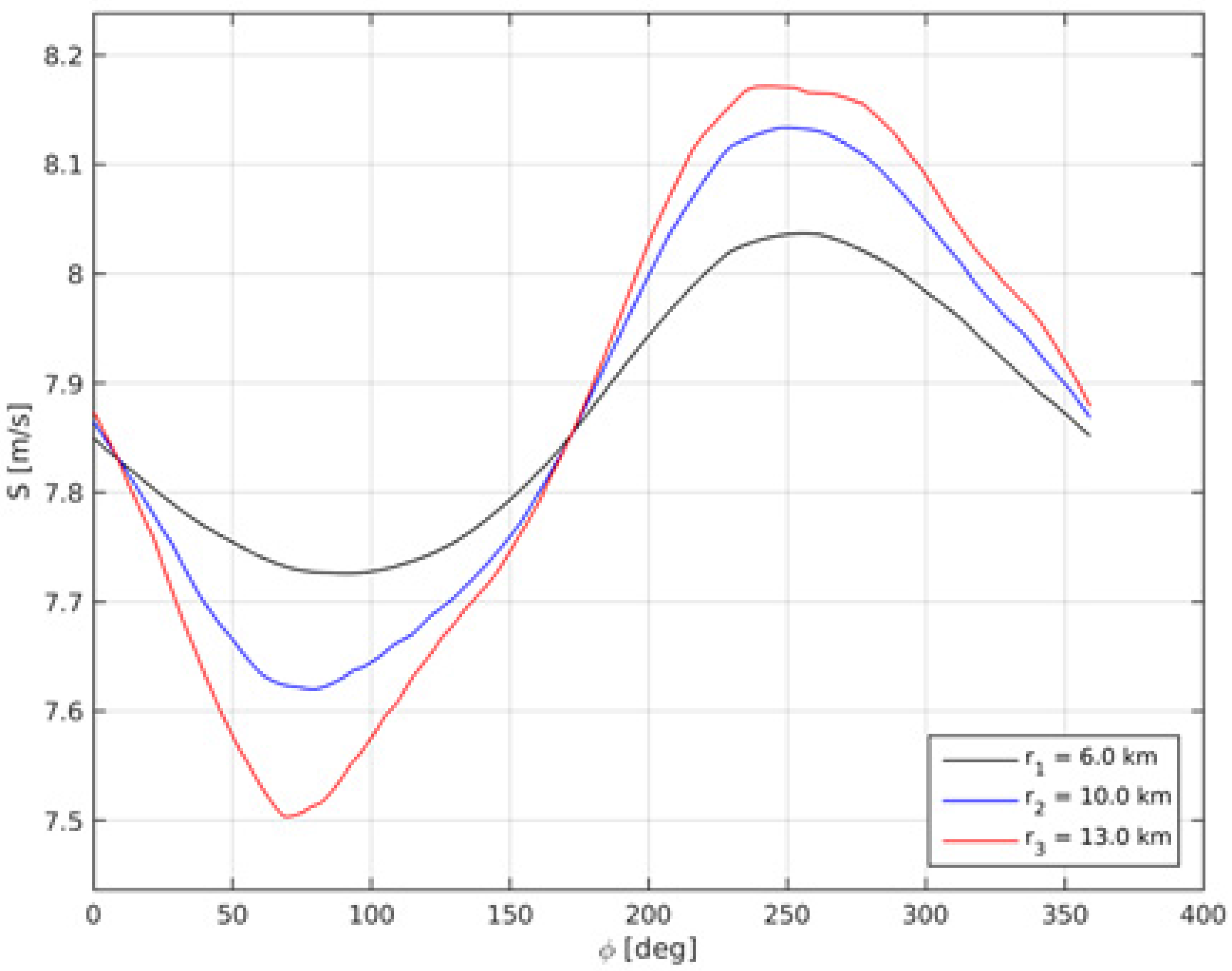
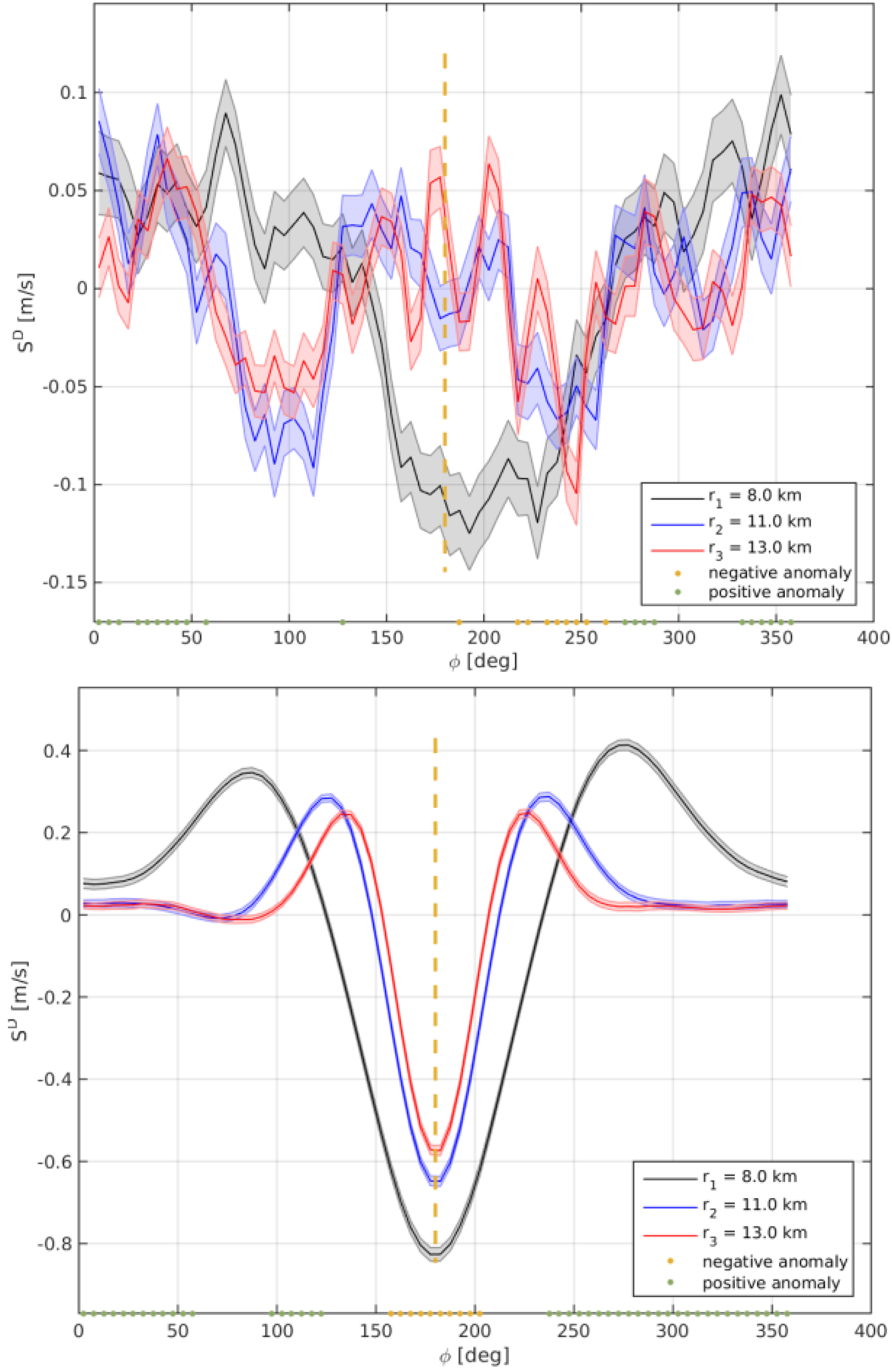
5.2. PARK Model Results

The PARK model is used to simulate 855 cases (a few more cases than used above but the results are expected to be comparable) at Horns Rev 1. The SAR wind time series at 10 m is used as input, the winds are extrapolated to 70 m and the wake is modeled at that height and finally the winds are extrapolated downwards to 10 m again. The extrapolation is done using the logarithmic wind profile assuming a constant roughness length of 0.0002 m. The results are presented at 10 m. Three wake decay coefficients are used. The three wake decay coefficients are: 0.03, 0.04 and 0.05. The wake decay coefficient 0.04 is often used offshore while the lower and higher values are used in case of more stable or unstable cases. The results are rotated and averaged and the results are shown in Figure 11. The coastal gradient is not accounted for in the PARK model results. In case the coastal gradient should be added in the PARK model this could either be from SAR or from WRF, but it has not been attempted in the current study. The results are comparable to the wake wind speed deficit (S^D) results.

Figure 11. Wake results from the modified PARK model at Horns Rev 1 using wake decay coefficients (a) 0.03; (b) 0.04 and (c) 0.05.

Figure 11. Wake results from the modified PARK model at Horns Rev 1 using wake decay coefficients (a) 0.03; (b) 0.04 and (c) 0.05.

Figure 11 shows the systematic variation in wake with deeper wakes at the inner radius and progressively weaker wakes further from the wind farm. The wake decay coefficient of 0.03 gives much deeper wakes than for the higher wake decay coefficients, in particular for the inner radius. The shape of the wake compares well to Figure 10 from SAR and WRF.

5.3. Horns Rev 2 Results

Horns Rev 2 is located further offshore than Horns Rev 1 thus similar directional but lower wind speed gradients are expected. The mean wind speed gradient results based on SAR and WRF for Horns Rev 2 are presented in Figure 12a,b.The coastal wind speed gradient observations in SAR at Horns Rev 2 (Figure 12a) show a very peaked and significant minimum around 110° corresponding to the direction of Horns Rev 1. The feature (drop of around 0.2 m·s⁻¹) is observed at all radii (8, 11 and 13 km) and is most pronounced at the outer radius. This narrow fine-scale feature is only fully observed in SAR. SAR resolves features at smaller spatial scales than the WRF simulations presented here. This minimum value might be related to the wind farm wake from Horns Rev 1. Interestingly WRF shows a broad minimum with a shift in direction between radii from 100° at the 8 km radius to 110° at the 10 km radius and 120° at the 13 km radius (Figure 12b). Thus the WRF simulation may in fact here capture a blend of coastal gradient and wind farm wake from Horns Rev 1. At the western sector SAR shows a peaked maximum around 250° and similar wind speeds at all three radii while WRF shows flatter maximum and slightly higher winds at outer radii.

Figure 12c,d shows the rotated maps (S_rot) for Horns Rev 2. For SAR a minimum around 180° at 8 km radius is observed while at 10 km and 13 km the minima are around 250° and 110°, respectively. Only at 8 km do the WRF simulations agree with the SAR observations. The three radii at Horns Rev 2 are each located 2 km further from the wind farm center than the results for Horns Rev 1. This was necessary because the Horns Rev 2 wind farm is larger than the Horns Rev 1 wind farm. This however means that the wind alignment between inflow conditions and the deepest wind farm wake potentially deviate relatively more at Horns Rev 2 than Horns Rev 1.

Figure 12. Results for Horns Rev 2. (a) wind speed summations without rotation (mean wind speed gradient) (S) based on SAR; (b) WRF; (c) wind speed summations with rotation (S_rot) based on SAR; (d) WRF.

Figure 12. Results for Horns Rev 2. (a) wind speed summations without rotation (mean wind speed gradient) (S) based on SAR; (b) WRF; (c) wind speed summations with rotation (S_rot) based on SAR; (d) WRF.

Figure 13 shows the wake wind speed deficit (S^D) results from SAR and WRF. The results at the inner radius compare well even though the SAR results show a broader wake than WRF. Speed up in the side lobe winds are noticed both in SAR and WRF at the inner radii and no residual wind speed gradient is noted. At the middle and outer radii WRF shows gradual decrease in the wake winds speed deficit and speed up at the sides while the SAR results are difficult to interpret. In SAR the minimum wake wind speed deficit is not observed around 180° but around 100° and 250°. The analysis appears not to work so well in this case, in part due to the significant minimum around 110° in Figure 12a. This feature may possibly be the wake feature of Horn Rev 1, which acts to contaminate the analysis, as this feature can be as strong as the Horn Rev 2 wake itself.

Figure 13. Similar to Figure 10 but for Horns Rev 2.

Figure 13. Similar to Figure 10 but for Horns Rev 2.

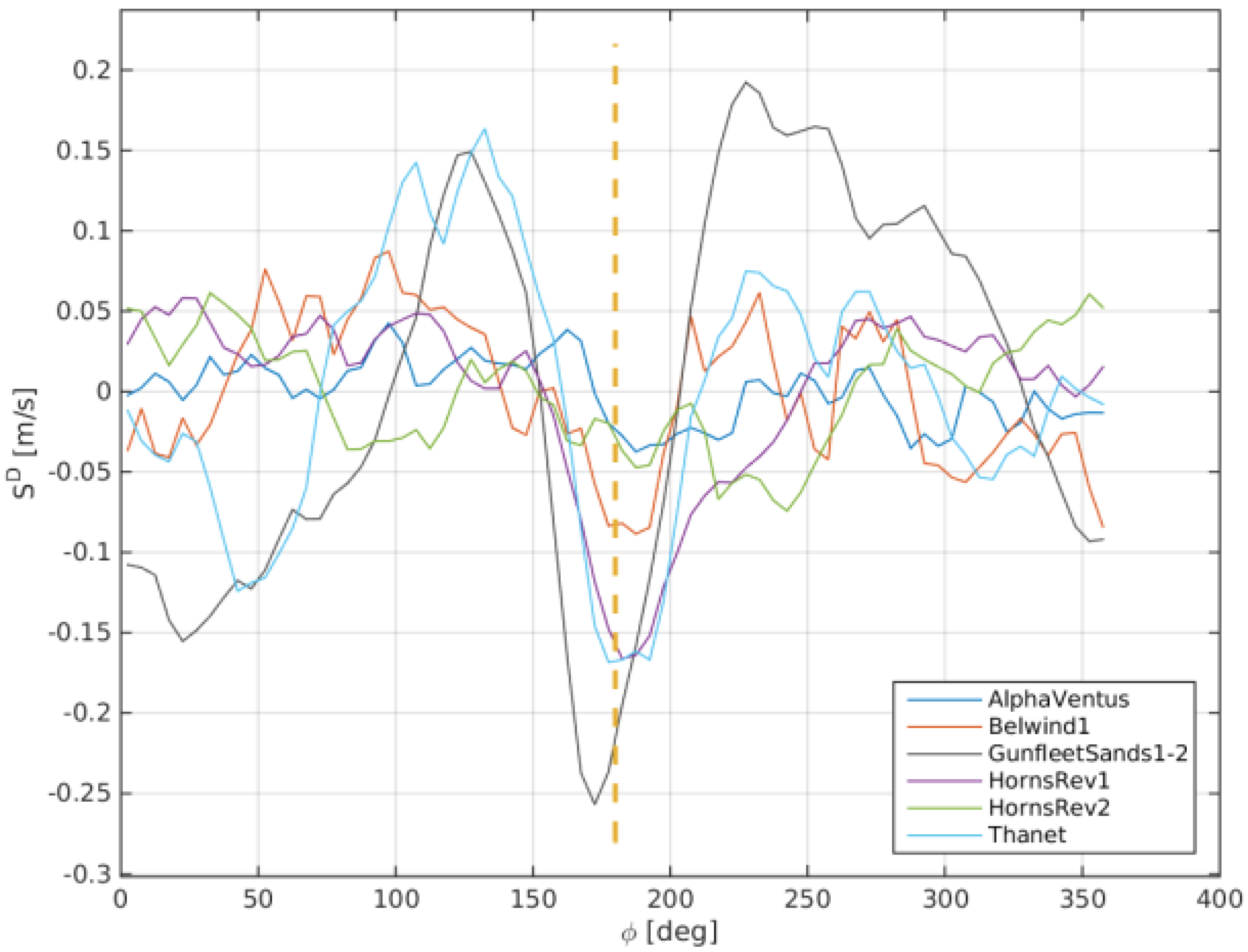
5.4. SAR-Based Results for Six Wind Farms

Based on the available Envisat ASAR wind field archive we find it interesting to compare the observed aggregated wind farm wakes at four other wind farms in the southern North Sea using the new methodology of rotation of the wind maps. The results of the wake wind speed deficit (S^D) are shown in Figure 14 together with the results from Horns Rev 1 and Horns Rev 2 already discussed.

It is the results for the average of the three radii (see Table 4) for each wind farm that is shown. Figure 14 shows results for six wind farms. It is noted that Gunfleet Sands 1 + 2 show the deepest wake wind speed deficit. The side lobe speed-up effects are clear. A residual wind speed gradient is not noted. For the wind speed summation (S) (not shown) there is a weaker signature of a climatological wind speed gradient across the wind farm compared to other wind farms, this may be because the radii used are smaller.

Figure 14. SAR-based wind farm wake observed at six wind farms, Alpha ventus, Belwind 1, Gunfleet Sands 1 + 2, Horns Rev 1, Horns Rev 2 and Thanet, showing the wake wind speed deficit (S^D).

Figure 14. SAR-based wind farm wake observed at six wind farms, Alpha ventus, Belwind 1, Gunfleet Sands 1 + 2, Horns Rev 1, Horns Rev 2 and Thanet, showing the wake wind speed deficit (S^D).

At the Thanet wind farm, the wake wind speed deficit results show very clear wake at around 180° and side lobe speed-up effects. A residual of the coastal wind speed gradient is noted. There is a feature at 50° with lower winds that would need further investigation.

At the Belwind 1 wind farm the wake wind speed deficit is clear but not as pronounced as for the Gunfleet Sands 1 + 2, Thanet and Horns Rev 1 results. Weak side lobe effects are observed at Belwind 1. A residual of coastal wind speed gradient is not noted in the wake wind speed deficit despite that strong coastal gradient mean wind speed gradient is found in the coastal gradient plot (S) (not shown).

Finally, at the Alpha ventus wind farm, the smallest wind farm in terms of installed capacity and area, there is observed wake wind speed deficit at around 180°. The wind farm wake is not as pronounced as for the larger wind farms investigated. This is expected due to the size of the wind farm. The coastal gradient is not observed in the result but is noted in the coastal wind speed gradient (S) (not shown).

6. Discussion

The very long wind farm wakes observed in the RADARSAT-2 scene have in qualitative terms successfully been modeled both by the PARK and WRF model at several wind farms in the southern North Sea. The comparison is qualitative due the different nature of data. The SAR-based results are near-instantaneous observations of the sea surface while wake model results are time-averaged results withbest representation of the conditions at around hub-height. Thus we focus on the apparent wind farm wake direction and the length of the wakesin this comparison instead of the wake deficit at any given location. The SAR image has the advantage of clear visible wake features. Thus the retrieved wind field can be used to evaluate the wake model results in qualitative terms.

We are interested in developing more robust SAR-based wind farm wake data representation for the evaluation of wake models. Therefore the climatology of wind farm wake is necessary. The Envisat ASAR data of wind fields enable us to study the wind farm wake at Horns Rev 1 and 2 with the data set divided into 12 wind directional bins. The results are compared to the PARK model. Occasionally good agreement is found but due to strong coastal wind speed gradients, bathymetry effects and too few samples firm conclusions cannot be drawn.

The new method, in which the wind field maps are rotated, overcomes two of the main issues when trying to isolate the wind farm effect of the wake on the wind fields: the low number of samples and the coastal gradient. The first advantage is that the inflow wind is aligned (rotated) with 1° bins instead of 30° bins. This gives more certainty that the deepest wind farm wake are overlapping in the aggregated results. With the inflow wind speed used to normalize the winds in the wake, the wake are clearly seen but at the same time a residual of the coastal gradient is often noted, e.g., at Horns Rev 1. The clearest wind farm wake results are typically obtained using the side lobe winds for normalization, the wake wind speed deficit method (S^D). This is not too surprising as the coastal wind speed gradients at most wind farms are significant and the circles used around the large offshore wind farms need to be at some distance. Therefore any inhomogeneity in the flow, most importantly the coastal gradient, but in fact also meandering and other atmospheric features gain importance. Also in [2] the nearby parallel transects winds along the wind farm wake were optimal for normalization, rather than the inflow winds upwind of the wind farm.

The number of samples at Horns Rev 2 is 303 while at Horns Rev 1 it is 835. So the lower number of samples at Horns Rev 2 could be one reason for the lesser clarity in data at this site when compared to Horns Rev 1. Also the influence of the Horns Rev 1 wind farm wake may hinder full interpretation at Horns Rev 2 in particular at radii far from the Horns Rev 2 wind farm. Finally it should be mentioned that the Horns Rev 1 wind farm has a geometric shape (turbine lay-out) more convenient for the proposed new methodology of analysis than that of the Horns Rev 2 wind farm. We assume that all wind turbines are in operation at all times a characteristic which may not be fulfilled.

The SAR-based aggregated wind farm wake data compare well both to the WRF simulations and the PARK model results. It is the first time that assessment of the wind farm wake climatology has been attempted based on SAR (to our knowledge) and the results are promising. The main importance of the establishment of SAR-based wake wind speed aggregated results is for the validation of wind farm wake models in the far-field wake region where other observations are extremely limited. In the future more wind farms will operate offshore thus cluster-scale wind farm wake therefore become an even more important focus area. It is suggested to continue this type of research using new SAR data from the Sentinel-1 mission.

7. Conclusions

The case study based on a RADARSAR-2 scene is a unique situation with fairly homogeneous flow across the southern North Sea. The observed wind farm wakes are visible in the SAR scene and thus appealing for demonstration. Both WRF and PARK reproduce the observed very long wind farm wakes convincingly regarding their direction and extent. SAR archive renders possible climatology studies.

The available Envisat ASAR data archive at Horns Rev is the most comprehensive. It has therefore been used for geo-located wind farm wake climatology studies. However the results are only occasionally clear for interpretation due to the limited number of samples per 30° sectors, the coastal wind speed gradient and oceanic bathymetry effects in SAR at Horns Rev.

The key results are based on a new methodology of rotating wind maps. By applying the new methodology to SAR-based wind fields, mesoscale model WRF and microscale model PARK results comparable aggregated wind farm wake results are obtained. The SAR-based findings strongly support the model results at Horns Rev 1. The new methodology increases the number of samples, aligns the wind direction of inflow much more accurately (1° bins) and in most cases but not always overcome the coastal wind gradient. The most convincing results are obtained for the wind wake deficit results in which the side lobe winds are used for normalization.

References

1. Christiansen, M.B.; Hasager, C.B. Wake effects of large offshore wind farms identified from satellite SAR. Remote Sens. Environ. 2005, 98, 251–268. [Google Scholar] [CrossRef]
2. Christiansen, M.B.; Hasager, C.B. Using airborne and satellite SAR for wake mapping offshore. Wind Energy 2006, 9, 437–455. [Google Scholar] [CrossRef]
3. Li, X.; Lehner, S. Observation of TerraSAR-X for Studies on Offshore Wind Turbine Wake in near and Far Fields. IEEE 2013, 5, 1757–1768. [Google Scholar] [CrossRef]
4. Hasager, C.B.; Vincent, P.; Husson, R.; Mouche, A.; Badger, M.; Peña, A.; Volker, P.; Badger, J.; Di Bella, A.; Palomares, A.; et al. Comparing satellite SAR and wind farm wake models. J. Phys. Conf. Ser. 2015, 625. in press. [Google Scholar]
5. Hasager, C.B.; Mouche, A.; Badger, M.; Bingöl, F.; Karagali, I.; Driessenaar, T.; Stoffelen, A.; Peña, A.; Longépé, N. Offshore wind climatology based on synergetic use of Envisat ASAR, ASCAT and QuikSCAT. Remote Sens. Environ. 2015, 156, 247–263. [Google Scholar] [CrossRef] [Green Version]
6. Quilfen, Y.; Chapron, B.; Elfouhaily, T.; Katsaros, K.; Tournadre, J. Observation of tropical cyclones by high-resolution scatterometry. J. Geophys. Res. 1998, 103, 7767–7786. [Google Scholar] [CrossRef]
7. Katic, I.; Højstrup, J.; Jensen, N.O. A simple model for cluster efficiency. In Proceedings of the European Wind Energy Association Conference & Exhibition, Rome, Italy, 7–9 October 1986.
8. Mortensen, N.G.; Heathfield, D.N.; Myllerup, L.; Landberg, L.; Rathmann, O. Getting Started with WAsP 9; Tech. Rep. Risø-I-2571(EN); Risø National Laboratory: Roskilde, Denmark, 2007. [Google Scholar]
9. Jensen, N.O. A Note on Wind Generator Interaction; Tech. Rep. Risø-M-2411(EN); Risø National Laboratory: Roskilde, Denmark, 1983. [Google Scholar]
10. Skamarock, W.C.; Klemp, J.B.; Dudhia, J.; Gill, D.O.; Barker, D.M.; Duda., M.; Huang, X.Y.; Wang, W.; Powers, J.G. A description of the advanced research WRF version 3. Tech. Rep. 2008. [Google Scholar] [CrossRef]
11. Adams, A.S.; Keith, D.W. A wind farm parametrization for WRF. Available online: http://www2.mmm.ucar.edu/wrf/users/workshops/WS2007/abstracts/5-5_Adams.pdf (accessed on 2 June 2015).
12. Baidya Roy, S. Simulating impacts of wind farms on local hydrometeorology. J. Wind Eng. Ind. Aerodyn. 2011, 99, 491–498. [Google Scholar] [CrossRef]
13. Blahak, U.; Goretzki, B.; Meis, J. A simple parametrisation of drag forces induced by large wind farms for numerical weather prediction models. In Proceedings of the European Wind Energy Conference & Exhibition 2010 (EWEC), Warsaw, Poland, 20–23 April 2010.
14. Jacobson, M.Z.; Archer, C.L. Saturation wind power potential and its implications for wind energy. Proc. Natl. Acad. Sci. USA 2012, 109, 15679–15684. [Google Scholar] [CrossRef] [PubMed]
15. Fitch, A.; Olson, J.; Lundquist, J.; Dudhia, J.; Gupta, A.; Michalakes, J.; Barstad, I. Local and mesoscale impacts of wind farms as parameterized in a mesoscale NWP model. Mon. Weather Rev. 2012, 140, 3017–3038. [Google Scholar] [CrossRef]
16. Volker, P.J.H.; Badger, J.; Hahmann, A.H.; Ott, S. The Explicit Wake Parametrisation V1.0: A wind farm parametrisation in the mesoscale model WRF. GMDD 2015, 8, 3481–3522. [Google Scholar] [CrossRef] [Green Version]
17. Nakanishi, M.; Niino, H. Development of an improved turbulence closure model for the atmospheric boundary layer. J. Meteorol. Soc. Jpn. 2009, 87, 895–912. [Google Scholar] [CrossRef]
18. Kain, J.S. The Kain-Fritsch convective parameterization: An update. J. Appl. Meteorol. Climatol. 2004, 43, 170–181. [Google Scholar] [CrossRef]
19. Thompson, G.; Field, P.R.; Rasmussen, M.; Hall, W.D. Explicit forecasts of winter precipitation using an improved bulk micro- physics scheme. Part II: Implementation of a new snow parameterization. Mon. Weather Rev. 2008, 136, 5095–5115. [Google Scholar] [CrossRef]
20. Mlaver, E.J.; Taubman, S.J.; Brown, P.D.; Iacono, M.J.; Clough, S.A. Radiative transfer for inhomogeneous atmosphere: RRTM, a validated corrected-k model for the long wave. J. Geophys. Res. 1997, 102, 16663–16682. [Google Scholar]
21. Dudhia, J. Numerical study of convection observed during the wind monsoon experiment using a mesoscale two-dimensional model. J. Atmo. Sci. 1989, 46, 3077–3107. [Google Scholar] [CrossRef]
22. Chen, F.; Dudhia, J. Coupling an advanced land surface-hydrology model with the Penn State-NCAR MM5 modeling system. Part I: Model implementation and sensitivity. Mon. Weather Rev. 2001, 129, 569–585. [Google Scholar] [CrossRef]
23. Uppala, S.M.; Kallberg, P.W.; Simmons, A.J.; Andrae, U.; Bechtold, V.; Fiorino, M.; Gibson, J.K.; Haseler, J.; Hernandez, A.; Kelly, G.A.; et al. The ERA-40 re-analysis. Quart. J. R. Meteorol. Soc. 2005, 131. [Google Scholar] [CrossRef]
24. Barthelmie, R.J.; Badger, J.; Pryor, S.C.; Hasager, C.B.; Christiansen, M.B.; Jørgensen, B.H. Offshore coastal wind speed gradients: Issues for the design and development of large offshore windfarms. Wind Eng. 2007, 31, 369–382. [Google Scholar] [CrossRef]