
Evaluation of a Blade Force Measurement System for a Vertical Axis Wind Turbine Using Load Cells

 ,
,
Abstract
:
1. Introduction
2. Theory
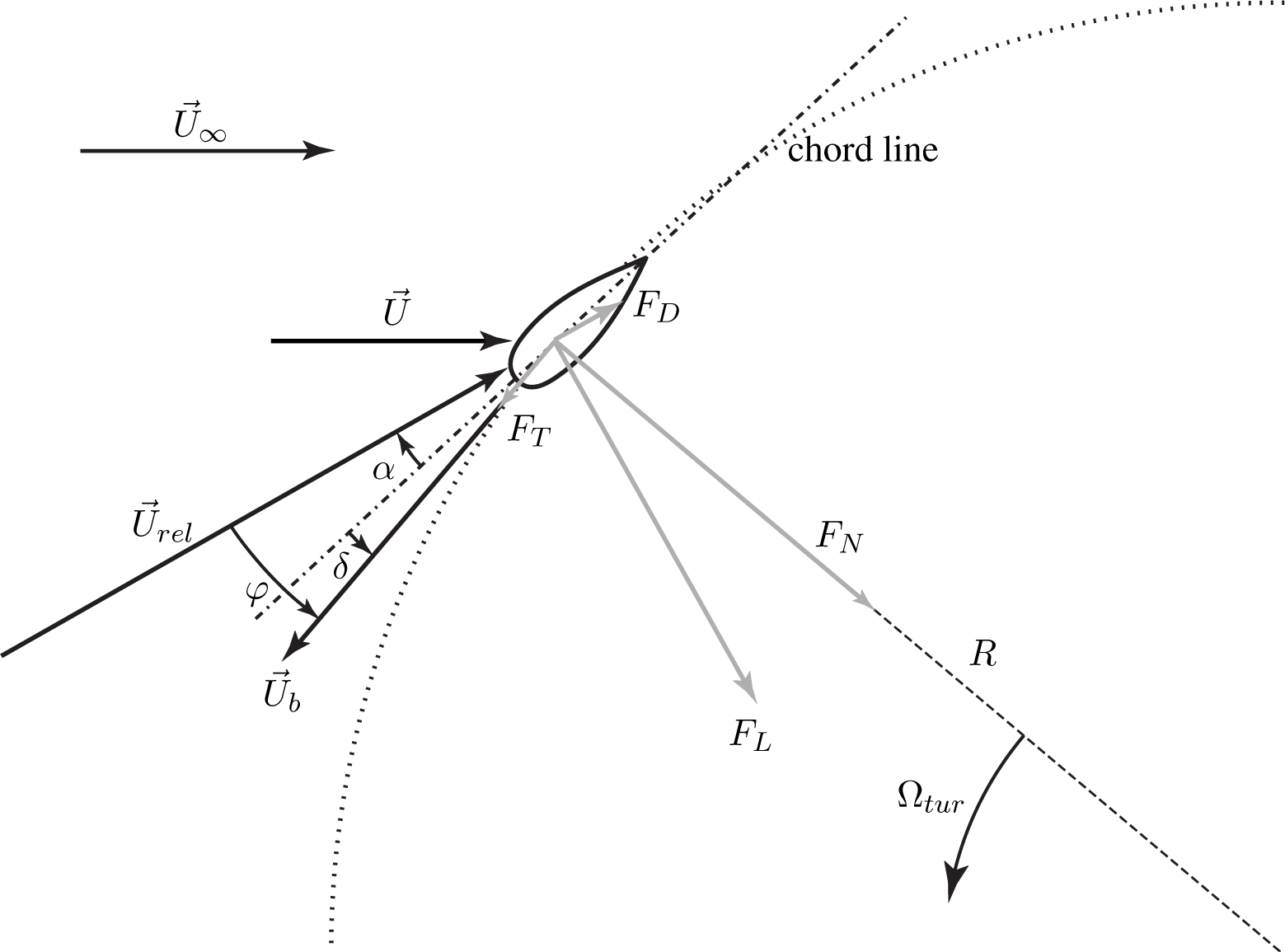
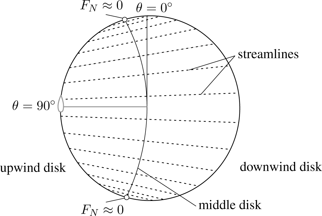
2.1. Aerodynamic Blade Forces
2.2. Turbine Torque
2.3. Aerodynamic Simulation Model
3. Method
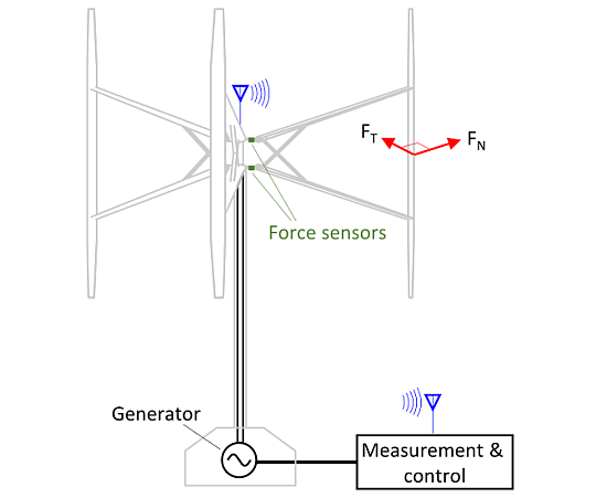
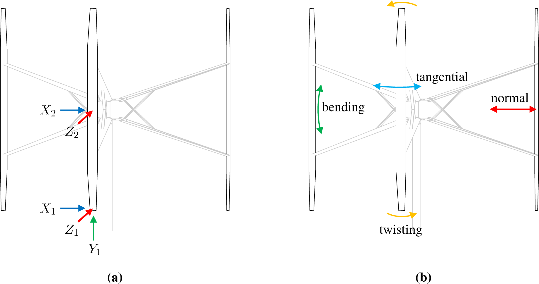
3.1. Blade Forces
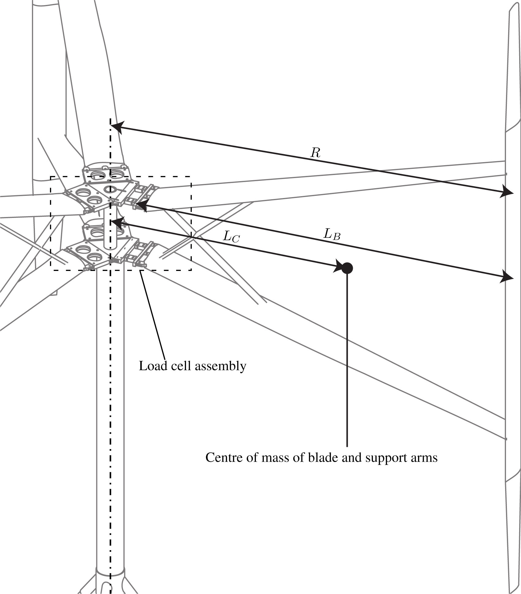
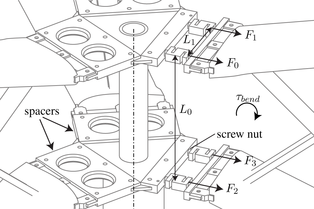
3.2. Load Cells
3.3. Turbine
3.4. Generator and Shaft
3.5. Weather and Site Conditions
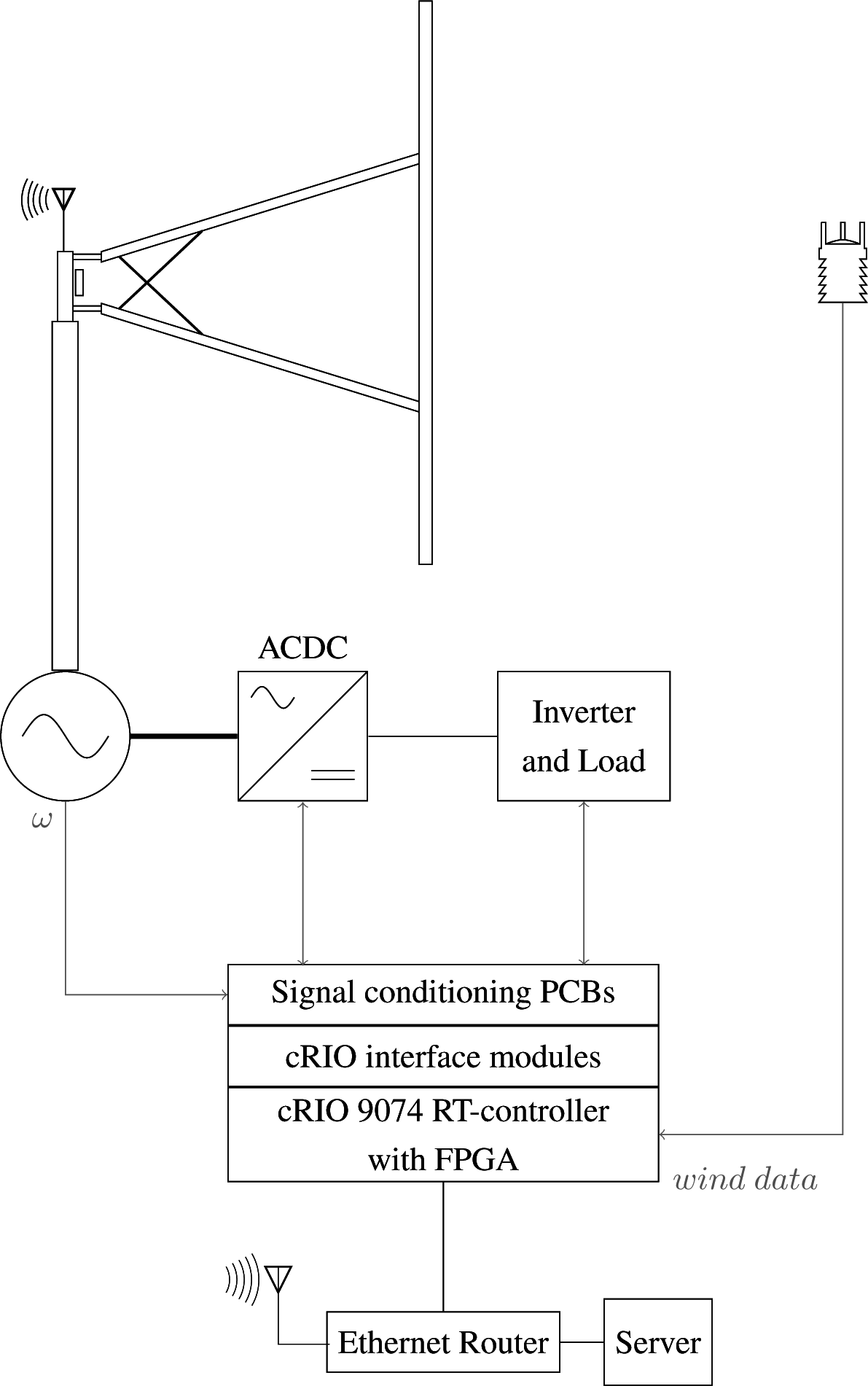
3.6. Control and Data Acquisition
3.7. Blade Position
3.8. Error Estimation Method
3.9. Experimental Procedure
4. Results and Discussion
4.1. Influence of Load Cells on the Turbine Dynamics
4.2. Accuracy
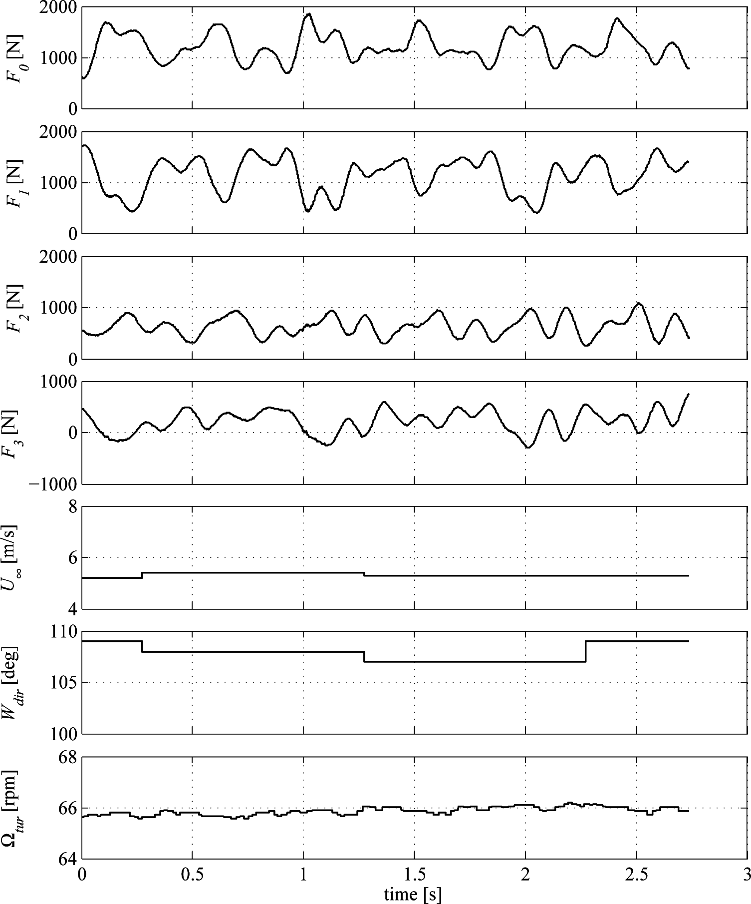
4.3. System Output and Performance
4.4. Radial and Normal Force
4.5. Tangential Force and Torques
4.6. General Discussion
5. Conclusions
Nomenclature
| ∆ | Maximum error of parameter |
| α deg | Angle of attack |
| δ deg | Pitch angle |
| φ deg | Angle of the relative wind |
| θ deg | Azimuth angle |
| F0 | N Load Cell 0 force |
| F1 | N Load Cell 1 force |
| F2 | N Load Cell 2 force |
| F3 | N Load Cell 3 force |
| F0,zero | N Load Cell 0 no-load force |
| F1zero | N Load Cell 1 no-load force |
| F2zero | N Load Cell 2 no-load force |
| F3zero | N Load Cell 3 no-load force |
| FB,LC | N Bending force load cell input offset removed |
| FB,zero | N Bending force zero value |
| FD | N Drag force |
| FL | N Lift force |
| FN | N Aerodynamic normal force |
| FN,zero | N Aerodynamic normal force zero value |
| FR | N Radial force |
| FT | N Tangential force |
| FT,LC | N Tangential force load cell input offset removed |
| FTzero | N Tangential force zero value |
| g m s2 | Local gravity |
| h %RH | Air humidity |
| λ | Tip speed ratio (TSR) |
| L0 m | Vertical distance between sensors |
| L1 m | Horizontal distance between sensors |
| LB m | Distance sensors to blade |
| LC m | Distance load cells to center of mass |
| m kg | Mass of blade and support arms |
| nB | Number of blades |
| Ωtur rad/s | Turbine rotational speed |
| Ωtur,rpm rpm | Turbine rotational speed (rpm) |
| p Pa | Barometric pressure |
| R m | Turbine radius |
| ρ kg/m3 | Air density |
| T °C | Air temperature |
Unit vector in tangential direction | |
| τbend Nm | Bending moment of the blade |
| τB Nm | Blade torque |
| 〈τB〉rev Nm | Blade torque, average over full revolutions |
| τtur Nm | Turbine torque, average over full revolutions |
| m/s | Wind speed |
| U∞ m/s | Wind speed magnitude,
|
| m/s | Speed of blade |
| m/s | Wind speed at blade |
| m/s | Relative wind |
| Wdir deg | Wind direction |
Acknowledgments
Author Contributions
Conflicts of Interest
References
- Sutherland, H.J.; Berg, D.E.; Ashwill, T.D. A retrospective of VAWT technology. In Technical Report SAND2012-0304; Sandia National Laboratories: Albuquerque, NM, USA, 2012. [Google Scholar]
- Johnston, S.F. Proceedings of the Vertical Axis Wind Turbine (VAWT) Design Technology Seminar for Industry. In Technical Report SAND80-0984; Sandia National Laboratories: Albuquerque, NM, USA, 1980. [Google Scholar]
- Akins, R.E. Measurements of Surface Pressures on an Operating Vertical-Axis Wind Turbine. In Technical Report SAND89-7051; Sandia National Laboratories: Albuquerque, NM, USA, 1989. [Google Scholar]
- Oler, J.; Strickland, J.; Im, B.; Graham, G. Dynamic stall regulation of the Darrieus turbine. In Technical Report SAND83-7029; Sandia National Laboratories: Albuquerque, NM, USA, 1983. [Google Scholar]
- Ahmadi-Baloutaki, M.; Carriveau, R.; Ting, D.S.K. Straight-bladed vertical axis wind turbine rotor design guide based on aerodynamic performance and loading analysis. Proc. Inst. Mech. Eng. Part A J. Power Energy 2014, 228, 742–759. [Google Scholar]
- Ferrari, G. Development of an Aeroelastic Simulation for the Analysis of Vertical-Axis Wind Turbines. Ph.D. Thesis, The University of Auckland, Auckland, New Zealand, 2012. [Google Scholar]
- Shires, A. Development and Evaluation of an Aerodynamic Model for a Novel Vertical Axis Wind Turbine Concept. Energies 2013, 6, 2501–2520. [Google Scholar] [Green Version]
- Dyachuk, E.; Goude, A. Simulating Dynamic Stall Effects for Vertical Axis Wind Turbines Applying a Double Multiple Streamtube Model. Energies 2015, 8, 1353–1372. [Google Scholar]
- Kjellin, J.; Bernhoff, H. Electrical starter system for an H-rotor type VAWT with PM-generator and auxiliary winding. Wind Eng. 2011, 35, 85–92. [Google Scholar]
- Solum, A.; Deglaire, P.; Eriksson, S.; Stålberg, M.; Leijon, M.; Bernhoff, H. Design of a 12 kW vertical axis wind turbine equipped with a direct driven PM synchronous generator, Proceedings of the EWEC 2006-European wind Energy Conference & Exhibition, Athens Greece, 27 February–2 March 2006.
- Deglaire, P.; Eriksson, S.; Kjellin, J.; Bernhoff, H. Experimental results from a 12 kW vertical axis wind turbine with a direct driven PM synchronous generator, Proceedings of the EWEC 2007-European Wind Energy Conference & Exhibition, Milan, Italy, 7–10 May 2007.
- Kjellin, J.; Eriksson, S.; Deglaire, P.; Bülow, F.; Bernhoff, H. Progress of control system and measurement techniques for a 12 kW vertical axis wind turbine, Proceedings of the EWEC 2008-European Wind Energy Conference & Exhibition, Brüssels, Belgium, 31 March–3 April 2008.
- Eriksson, S.; Solum, A.; Leijon, M.; Bernhoff, H. Simulations and experiments on a 12 kW direct driven PM synchronous generator for wind power. Renew. Energy 2008, 33, 674–681. [Google Scholar]
- Kjellin, J.; Bülow, F.; Eriksson, S.; Deglaire, P. Power coefficient measurement on a 12 kW straight bladed vertical axis wind turbine. Renew. Energy 2011, 36, 3050–3053. [Google Scholar]
- Sheldahl, R.E.; Klimas, P.C. Aerodynamic characteristics of seven symmetrical airfoil sections through 180-degree angle of attack for use in aerodynamic analysis of vertical axis wind turbines. In Technical Report SAND80-2114; Sandia National Laboratories: Albuquerque, NM, USA, 1981. [Google Scholar]
- Halldin, S.; Bergström, H.; Gustafsson, D.; Dahlgren, L.; Hjelm, P.; Lundin, L.C.; Mellander, P.E.; Nord, T.; Jansson, P.E.; Seibert, J.; et al. Continuous long-term measurements of soil-plant-atmosphere variables at an agricultural site. Agric. For. Meteorol. 1999, 98–99, 75–102. [Google Scholar]
- Power performance measurements of electricity producing wind turbines. In Technical Report IEC 61400-12-1:2005(E); International Electrotechnical Commission: Geneva, Switzerland, 2005.
- Bohn, C.; Atherton, D.A. Analysis package comparing PID anti-windup strategies. IEEE Control Syst. Mag. 1995, 15, 34–40. [Google Scholar]


| Measured Parameter | Value | Maximum Error |
|---|---|---|
| Turbine radius, R | 3.24 m | ±0.01 m |
| Center of mass, LC | 1.83 m | ±0.01 m |
| Distance sensor to blade, LB | 2.99 m | ±0.01 m |
| Vertical distance between sensors, L0 | 0.500 m | ±0.005 m |
| Horizontal distance between sensors, L1 | 0.200 m | ±0.0005 m |
| Mass of blade and support arms, m | 35.79 kg | ±0.05 kg |
| Turbine speed, Ωtur | ±0.05 rpm |
| Characteristic | Original | With Load Cells |
|---|---|---|
| Power | 12 kW | |
| Rotational speed | 127 rpm | |
| Rated blade tip speed | 40 m/s | |
| Rated wind speed | 12 m/s | |
| Number of blades | 3 | |
| Hub height | 6 m | |
| Swept area | 30 m2 | 32 m2 |
| Turbine radius, R | 3 m | 3.2 m |
| Blade length | 5 m | |
| Blade airfoil | NACA0021 | |
| Chord length | 0.25 m | |
| Tapering, linear | 1 m (from tip) | |
| Tip chord length | 0.15 m | |
| Blade pitch, δ | 2° | 2° |
| Measured Parameter | Max Error | Comments | |
|---|---|---|---|
| Wind speed | ΔU∞ = | ±0.3 m/s | at 0 m/s to 10 m/s |
| ±3 % | at 10 m/s to 35 m/s | ||
| Wind direction | ΔWdir = | ±3.0° | |
| Barometric pressure | Δp = | ±0.05 Pa | at 0 °C to 30 °C |
| ±0.1 Pa | at −52 °C to 60 °C | ||
| Air temperature | ΔT = | ±0.3 °C | |
| Air humidity | Δh = | ±3 %RH | at 0 %RH to 90 %RH |
| ±5 %RH | at 90 %RH to 100 %RH | ||
| Air density | Δρ = | ±0.0016 kg/m3 | calculated from Δp, ΔT, Δh |
| valid for T < 15 °C, h < 90 %RH | |||
| Mode | Blade 11 (Hz) | Blade 2 (Hz) | Blade 32 (Hz) | Excitation |
|---|---|---|---|---|
| Twisting | 5.6 | 6.7 | 7.3 | X1 |
| Tangential 1 | 8.0 | 9.1 | 9.1 | X2 |
| Tangential 23 | 28.8 | 29.6 | 36.1 | X2 |
| Bending 1 | 3.2 | 3.2 | 3.2 | Y1 |
| Bending 2 | 4.6 | 4.6 | 4.6 | X1 |
| Normal 14 | 13.5 | 13.2 | 12.6 | Z2 |
| Normal 24 | 20.7 | 20.7 | 18.7 | Z1 |
| Measured Parameter | Value | Maximum Error |
|---|---|---|
| FN,zero | 15 N | ΔFN,zero = ±7 N |
| FT,zero | 37 N | ΔFT,zero = ±18 N |
| FB,zero | 1960 N | ΔFB,zero = ±63 N |
| F0 | ΔF0 = ±2.2 N | |
| F1 | ΔF1 = ±5.9 N | |
| F2 | ΔF2 = ±4.2 N | |
| F3 | ΔF3 = ±4.1 N |
© 2015 by the authors; licensee MDPI, Basel, Switzerland This article is an open access article distributed under the terms and conditions of the Creative Commons Attribution license (http://creativecommons.org/licenses/by/4.0/).
Share and Cite
Rossander, M.; Dyachuk, E.; Apelfröjd, S.; Trolin, K.; Goude, A.; Bernhoff, H.; Eriksson, S. Evaluation of a Blade Force Measurement System for a Vertical Axis Wind Turbine Using Load Cells. Energies 2015, 8, 5973-5996. https://doi.org/10.3390/en8065973
Rossander M, Dyachuk E, Apelfröjd S, Trolin K, Goude A, Bernhoff H, Eriksson S. Evaluation of a Blade Force Measurement System for a Vertical Axis Wind Turbine Using Load Cells. Energies. 2015; 8(6):5973-5996. https://doi.org/10.3390/en8065973
Chicago/Turabian StyleRossander, Morgan, Eduard Dyachuk, Senad Apelfröjd, Kristian Trolin, Anders Goude, Hans Bernhoff, and Sandra Eriksson. 2015. "Evaluation of a Blade Force Measurement System for a Vertical Axis Wind Turbine Using Load Cells" Energies 8, no. 6: 5973-5996. https://doi.org/10.3390/en8065973