Novel Segmentation Technique for Measured Three-Phase Voltage Dips

Abstract

This paper focuses on issues arising from the need to automatically analyze disturbances in the future (smart) grid. Accurate time allocation of events and the sequences of events is an important part of such an analysis. The performance of a joint causal and anti-causal (CaC) segmentation method has been analyzed with a set of real measurement signals, using an alternative detection technique based on a cumulative sum (CUSUM) algorithm. The results show that the location in time of underlying transitions in the power system can be more accurately estimated by combining CaC segmentation methods.

1. Introduction

The automatic analysis of power-system voltages and currents is an important part of the trend toward a future power system (also known as “the smart grid”) that enables, among other things, a much higher penetration of renewable electricity production. Automatic analysis of such data has been common practice in so-called power-quality monitors for the last 30 years or so [1]. The concept of power quality (PQ) [2,3,4,5] is closely related to grid efficiency and electricity production. Most PQ monitors limit themselves, however, to analysis based on the international standard on power-quality monitoring, IEC 61000-4-30, which defines a set of parameters to quantify both voltage quality and current quality. Next to this, a large volume of work has been published on more advanced signal-processing tools for extracting features and finding information about the underlying event or phenomenon causing a certain power-quality disturbance.

The complete and detailed supervision of power-quality disturbances would entail the following stages: detection, segmentation, and characterization. The complete characterization of a disturbance is needed to assess its cause, to prevent harmful effects on power system components, and to establish limits of responsibilities between a network’s operator and its final customers. All of these, in turn, are important building blocks toward the future power system, in which a substantially larger amount of renewable electricity production will be connected.

A substantial number of advanced signal-processing methods have been applied to detect and analyze PQ disturbances with satisfactory results (see [6,7] for an overview). According to [7], these methods can be grouped in time-dependent waveforms features [8], signal transformation [9], and parametric models [7]. For example, there are research studies based on using multiresolution generalized S-transform to detect disturbances [10].

A range of features can be extracted using advanced signal-processing methods. This work concentrates on the detection of a sudden change in the character of a waveform. Such a sudden change will typically be a change in magnitude of the voltage or current waveform, but it may also be a sudden change in distortion. For the detection of such a change, a detection parameter (DP) is compared to a threshold. When the DP exceeds the threshold, the system detects the change and starts a number of additional processing, communication and/or storage algorithms. It is necessary to establish a correct threshold value in order to obtain an appropriate trade-off between missing events (e.g., a change in waveform character that was not detected) and false alarms (e.g., the DP exceeds the threshold when there is no change in waveform character). An example of optimized threshold setting, by performing an analysis of the detection method using different values, is shown in [8].

This paper will concentrate on one specific type of change in waveform character: the “voltage dip”, a short-duration reduction of voltage magnitude. Such a dip can be due to a fault in the system, a motor starting or a transformer energizing. As faults are the most serious events occurring in a power system—potentially threatening its reliability and stability—extracting information from voltage dips is of special importance.

The aims of this paper are twofold: first, to develop an algorithm for fast detection of the start of voltage dips; and second, to study and further develop an algorithm to accurately locate the time instants of individual changes in the system associated with the dip. Those changes include fault initiation, the development of the fault, and fault clearing. The former algorithm uses the cumulative sum (CUSUM) method as a statistical estimator to determine the DP and the threshold (Section 2.1.3); the latter algorithm uses the causal and anti-causal (CaC) segmentation method introduced by [11]. The latter study suggests a statistically-based method to determine the threshold of DP and a CaC method to locate boundary points between transition and event segments. The performance of the method has been quantified using synthetic voltage waveforms [11] but has not been applied by any author to large numbers of measured voltage waveforms. In this work, CaC method is analyzed with several voltage-dip recordings obtained at different locations in medium-voltage networks.

The rest of this paper is organized as follows. An introduction of the method proposed for detection of dips is presented in Section 2: in Section 2.1, the CUSUM algorithm is proposed as a statistical estimator to determine the DP and the threshold; in Section 2.2, the CaC methodology is presented; and Section 2.3 presents a full overview of the proposed method. Section 3 studies the performance of the method in the detection of a multistage dip. Finally, the conclusions are given in Section 4.

2. Methodology

In this section, a modified version of the CaC segmentation described by [11] is presented as an efficient solution for correctly identifying non-stationary and quasi-stationary states in measured voltage waveforms. A total of one hundred recording files of dip events are available to this end; these are categorized according to the ABC classification [12]. These signals are events recorded by PQ instruments and contain both pre-trigger and post-trigger information.

To segment a waveform using the CaC algorithm, the initial use of a statistical estimator to determine the threshold of the DP is necessary. The transition boundary segments are established according to the results after applying the segmentation, using both a causal analysis window and an anti-causal analysis window.

2.1. Detection Algorithm

The model to detect a signal transition can be divided into three steps: signal modelling, setting the DP, and decision-making. The basic principle of signal modelling is the generation of residuals obtained from the comparison of actual and expected responses of the system using mathematical models. These residuals are expected to be zero (or zero mean) under no-fault conditions. In practical situations, the residuals are corrupted by the presence of noise, unknown disturbances, and uncertainties in the system model; the aim of the method is to generate robust residuals that are insensitive to noise and uncertainties while sensitive to faults. To this end, the filtering method was considered. In residual generation, an adaptive filter takes the measured signal and transforms it into a sequence of residuals that are similar to white noise before the change occurs. The filtering approach is used to separate the signal and the noise. For this purpose, finite impulse response (FIR) or infinite impulse response (IIR) filters can be used, designed by any standard method (Butterworth, Chebyshev, etc.) [13]. Regarding the DP step, the aim is to conduct the treatment of residuals using a statistical algorithm to determine if the residuals significantly deviate from zero. To evaluate whether or not the deviation of DP is significant, the DP values are compared with a threshold in the decision-making step.

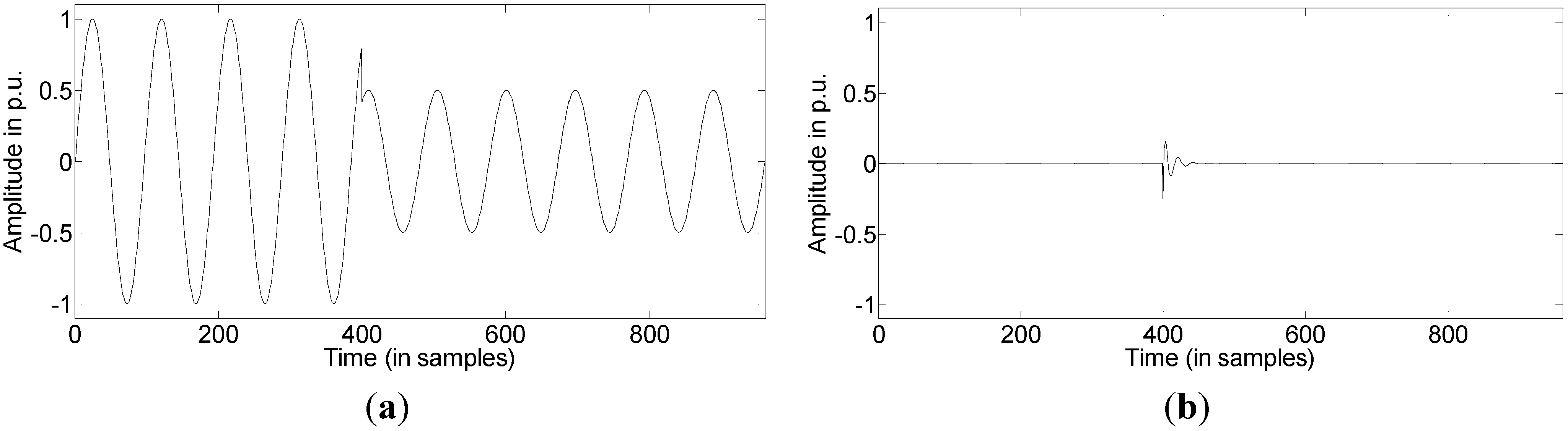
2.1.1. Signal Modelling Based on Filtering

In Le’s work [11], the square mean error (SME) method was used in the residual generation phase, but in the research with the real events, it was rejected because it was very sensitive to noise. In this work, a high-pass Butterworth filter was used to generate residuals. The Butterworth filter is an example of an all-pole filter with no ripple in the pass band, and is the best compromise between attenuation and phase response. This filter is sometimes called a “flat filter” due to the absence of ripples in the pass band and the stop band. Its transfer function is given by Equation (1):

|H|² = 1/(1 + (ω/ω_c)²ⁿ)

(1)

where n is the order of the filter and ω_c is the cutoff frequency. For this work, a 5th-order high-pass Butterworth filter has been used with a cutoff frequency of 3600 Hz for data sampled at 4800 Hz.

Figure 1 shows an example of residuals generation based on the results of the Butterworth filter. To do this, a synthetic disturbance is obtained by multiplying a synthetic signal with a step function. The magnitude of the step function drops from 1 pu to 0.5 pu at sample number 400. Figure 1a shows the resulting synthetic disturbance and Figure 1b shows the residual sequence of the filter.

Figure 1. (a) Synthetic transition signal; and (b) residual sequence from a Butterworth filter.

Figure 1. (a) Synthetic transition signal; and (b) residual sequence from a Butterworth filter.

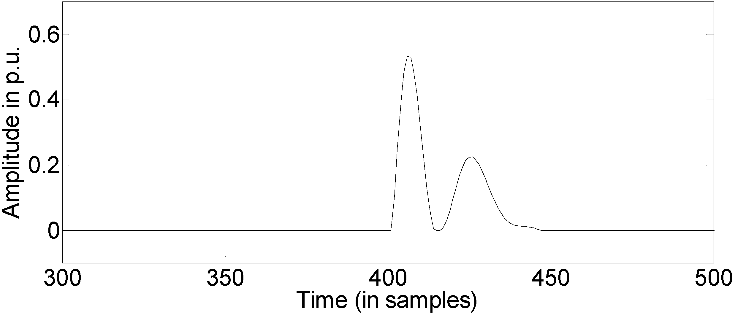
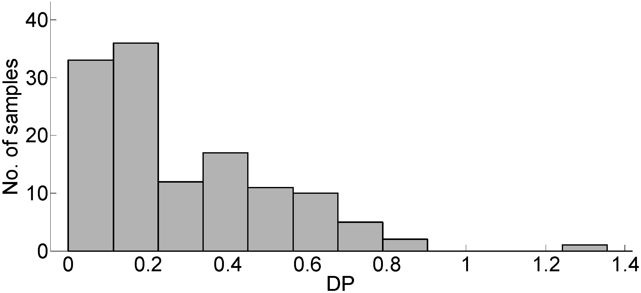
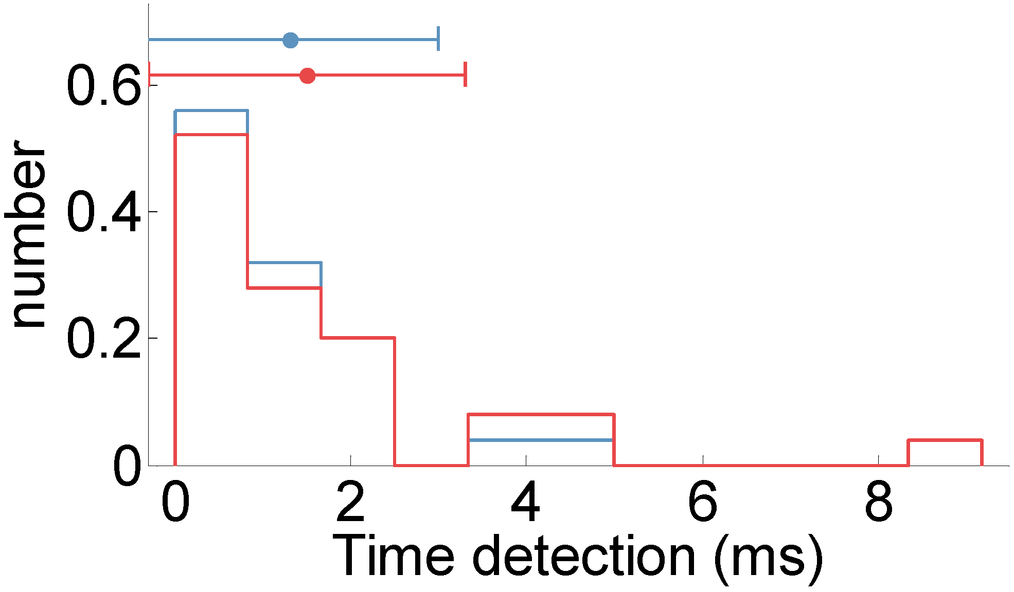
2.1.2. Detection Parameter Algorithm Based on Cumulative Sum Theory

The next step is the treatment of residuals through a statistical algorithm; they must be treated to be transformed into a distance measure (DP) that quantifies the deviation from the no-change-in-waveform hypothesis. To this end, several approaches can be used: analysis of the mean or variance of the residuals, the square of the residuals, or other options based on probability ratios. Le’s work [11] was based on Kalman filter, now the statistical algorithm used to develop the mentioned change detector (DP) is based on the mean and variance of the residuals; it is the CUSUM. The change detection in CUSUM is labelled as a change in the mean of the filtered signal. Therefore, the CUSUM inputs are set with the residuals from the filter that was previously used. The CUSUM directly includes all the information in the sequence of the sample by plotting the cumulative sums of any deviation of the sample values from a target value. The CUSUM has been widely used today, across industries, to monitor deviations of a process with respect to a target value and also to find evidence of change in the mean of a process. It has been successfully employed in power system fault detection in particular [14,15]. The CUSUM method is easy to handle and useful for detecting the locations of change points. The combination of information from several samples makes the CUSUM a suitable method for detecting small changes in PQ events. The CUSUM version used in this research is the so-called tabular or two-sided CUSUM [16,17]; it was designed to detect high and low changes in mean processes, recording the cumulative sums of signal samples in two directions. In this paper, the DP proposed to detect disturbances is based only on the statistical estimator for detecting an increase in the mean, according to Equation (2):

g_t = max(g_t−1 + s_t – (μ₀ + K),0)

(2)

where the DP, which is named as g_t, sums the inputs s_t from the filter. In Equation (2), μ₀ is the ideal mean of the process control state; and K is the reference value. The reference value should be set such that it allows the detection of changes in waveform character. It is usually set to half of the difference between the value of the average target control state and the value of the average in which the process is considered out of control [16]. The constant value given by the sum of μ₀ and K is removed to preventive false alarms. In this work, μ₀ is set to the mean of the samples processed to the current time and K is configured as 0.5 times the standard deviation of the filtered signal.

Figure 2 shows an example of the DP calculated with the residual sequence from a high pass Butterworth filter (shown in Figure 1b) and the statistical estimator g_t given by Equation (2).

Figure 2. Resulting detection parameter (DP) obtained from Equation (2).

Figure 2. Resulting detection parameter (DP) obtained from Equation (2).

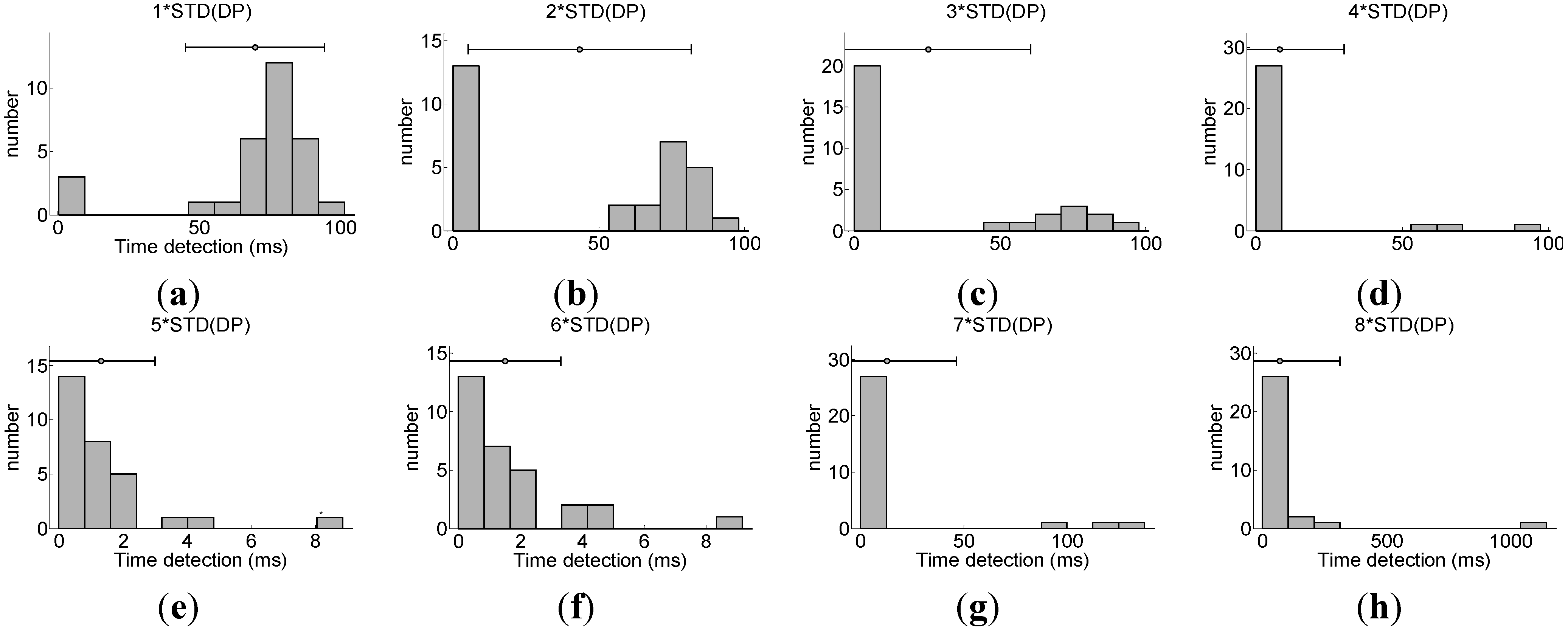
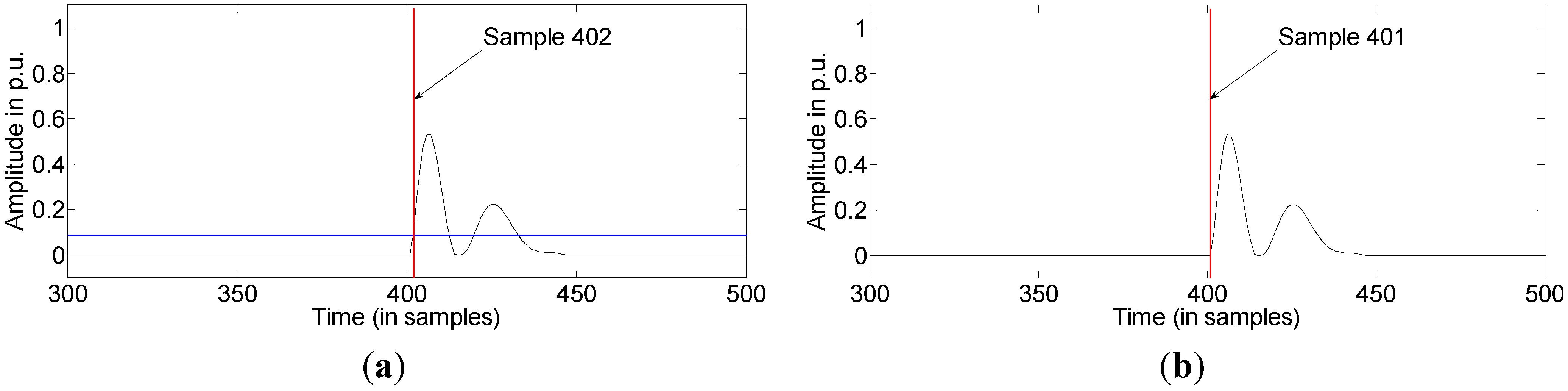
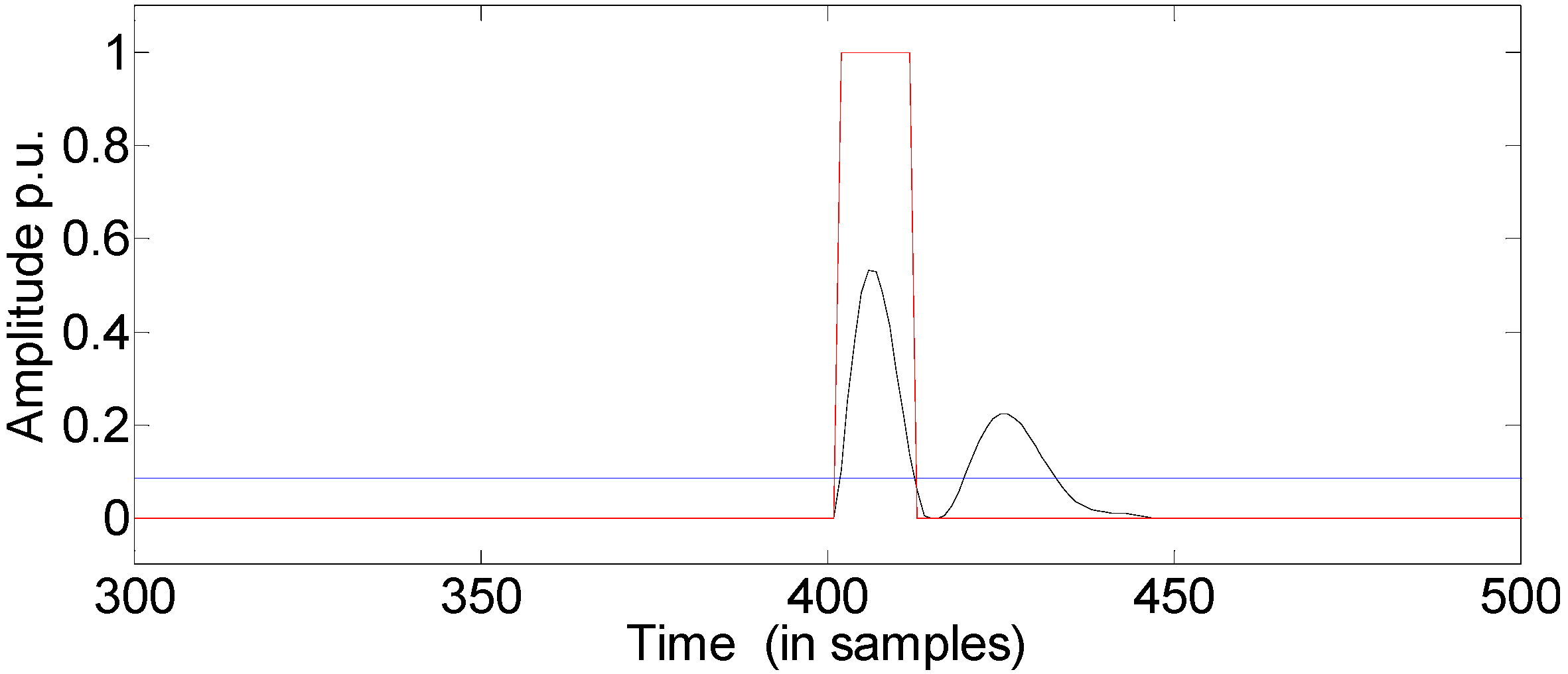
2.1.3. Decision-Making

The purpose of the decision-making phase is to detect when a process is considered to be out of control. In signal processing, the aim is to give an alarm when the value of a statistical parameter crosses a decision interval called threshold H. As mentioned above, non-zero residuals are generated if there is a disturbance in the signal processed (a change in waveform characteristics). This situation produces a change in the mean of the samples processed to the current time so that the change detection algorithm, DP, must indicate the variation. The main problem in statistical change detection is determining the optimal value of the threshold to obtain high accuracy of change detection and a low rate of false alarms.

To set a threshold H that avoids false alarms, 127 measured events were filtered and analyzed. Later, the CUSUM algorithm was used to get the DP, and the result was studied through a probability density function (PDF). Figure 3 shows the result of the PDF test; one can see that setting the threshold lower than the critical DP, zero value, increases the probability of the detection, but an increase in the number of false alarms is also produced due to the underlying noise of real measurements.

Thus, to avoid this problem and to design a robust detection algorithm, an adaptive threshold has been integrated with the proposed method. To obtain a robust threshold the variance of the DP should be considered; to this end, several tests were accomplished with different variance multiples, whose results are shown in Figure 4.

Figure 3. Results from designing the threshold over 127 disturbances.

Figure 3. Results from designing the threshold over 127 disturbances.

Figure 4. Histograms of standard deviation of DP using several multiples: (a) 1*STD(DP); (b) 2*STD(DP); (c) 3*STD(DP); (d) 4*STD(DP); (e) 5*STD(DP); (f) 6*STD(DP); (g) 7*STD(DP); and (h) 8*STD(DP).

Figure 4. Histograms of standard deviation of DP using several multiples: (a) 1*STD(DP); (b) 2*STD(DP); (c) 3*STD(DP); (d) 4*STD(DP); (e) 5*STD(DP); (f) 6*STD(DP); (g) 7*STD(DP); and (h) 8*STD(DP).

Figure 4 shows the PDF of the detection time, in milliseconds, of the first transition of 127 disturbances recorded. From the figures, it can be seen that there is a significant increment in the detection time when the DP is multiplied by low values, as in Figure 4a–c. In Figure 4d, better results are obtained but there are cases in which the detection time is too high. The same occurs in the two last cases, Figure 4g,h. Thus, the best response in terms of detection time is obtained when the standard deviation is multiplied by 5 or 6. As shown in Figure 4e,f, in the worst cases the detection time does not exceed 10 ms. Figure 5 compares the distribution obtained when the standard deviation is multiplied by 5 to that obtained when it is multiplied by 6. One can see that there are not significant differences between the two cases, but lower times are obtained when the variance of the standard deviation of DP is multiplied by 5.

In other respects an additional counter, called N, is used to reduce the effect of the analysis window and accurately calculate the start of the transitions. The N parameter, introduced by [16], estimates the first out-of-control instant of the process and indicates the number of consecutive times that the DP is non-zero after crossing H. Therefore, the N parameter can be used to estimate the time elapsed between the start of the underlying transition (S) and the detection instant (T). Then, the non-stationary state of the process is triggered as a result of subtracting N from the initially set trigger point T.

Figure 5. Overlap of the histograms of standard deviation of DP multiplied by 5 (blue line) and 6 (red line).

Figure 5. Overlap of the histograms of standard deviation of DP multiplied by 5 (blue line) and 6 (red line).

Figure 6 shows the stopping rule method for the synthetic signal shown in Figure 1a. The alarm is triggered when the DP across H in sample 402, as shown in Figure 6a. Finally, the non-stationary state of the process is triggered as a result of subtracting N from the initially set trigger point. The result of this method of dip detection is shown in Figure 6b.

Figure 6. Results of detection for the synthetic disturbance in Figure 1a: (a) the DP with the established threshold and trigger point; and (b) non-stationary detection.

Figure 6. Results of detection for the synthetic disturbance in Figure 1a: (a) the DP with the established threshold and trigger point; and (b) non-stationary detection.

From Figure 6a one may see that the trigger point (the vertical line) is initially set in the sample number 402. The out of control variable (N) resulting from CUSUM is set to 1. Thus, the start of the disturbance is finally triggered at the 401 sample—the vertical line in Figure 6b.

2.2. Segmentation Algorithm

Once a change is detected, it is possible to perform the segmentation. When the DP method indicates the dip start, an indication flag is triggered. This flag is reset when the DP falls below threshold H, as shown in Figure 7.

The values of the DP that cross the threshold less than one cycle after a detected transition are not considered as transitions. They considered effects of the previous transition detected.

Figure 7. Causal segmentation window.

Figure 7. Causal segmentation window.

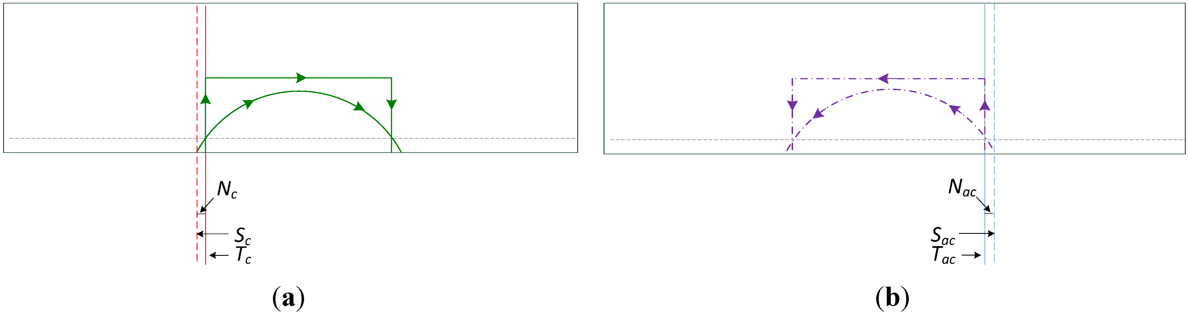
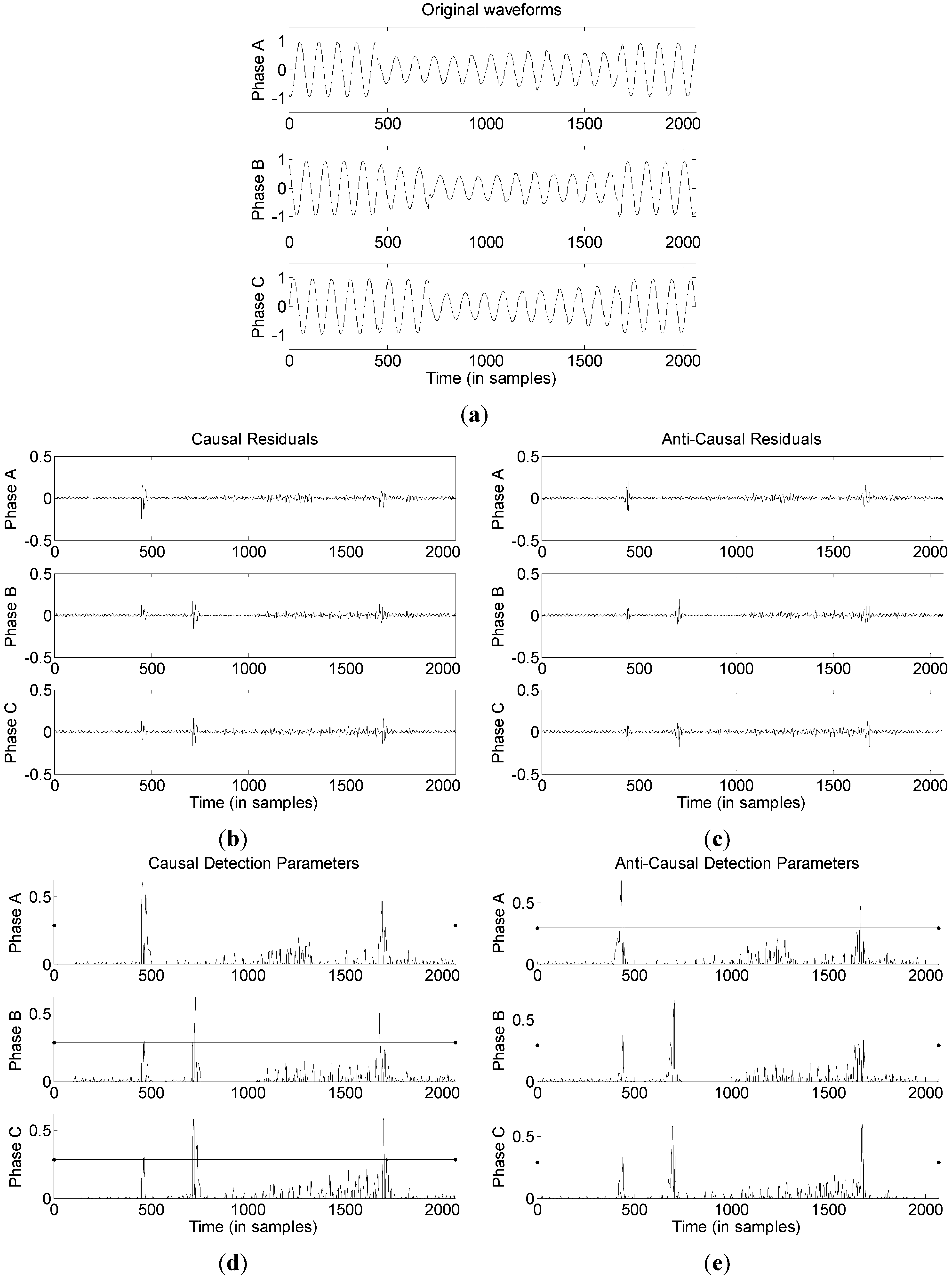
2.2.1. Causal and Anti-Causal Method

The following problem lies in the fact that there is always some detection delay due to the effect of the window used to calculate the detection index. A solution to this problem is the CaC method introduced by [11], which consists in applying, to a signal recorded of n samples, a joint segmentation scheme using a causal (forward time, from zero to nth sample) plus an anti-causal (backward time, from nth to zero sample) analysis window. The purpose of this method is to obtain an accurate time allocation of the underlying transition based on the results of the two analysis windows. It is proposed because conventional (causal) segmentation does not give an accurate trigger point but instead a delayed transition.

As discussed above, the out-of-control process point (causal flag T_c) is obtained from a causal analysis window. On CaC, a similar process takes place in both directions, introducing the opposite time direction; therefore, an anti-causal flag (T_ac) is also obtained. Then, the non-stationarity of the process in CaC directions, S_c and S_ac, is triggered as a result of subtracting N_c and N_ac from the initially set triggered points, T_c and T_ac, respectively, and given by the following equations:

S_c = T_c − N_c

(3)

S_ac = T_ac + N_ac

(4)

Figure 8 shows examples for causal segmentation (Figure 8a) and anti-causal segmentation (Figure 8b).

Figure 8. (a) Causal segmentation window; and (b) anti-causal segmentation window.

Figure 8. (a) Causal segmentation window; and (b) anti-causal segmentation window.

2.2.2. Estimation of the Signal Transitions Based on Causal and Anti-Causal Method

The classification of transitions as slow or fast is possible by considering the position of the CaC trigger flags (T_c, T_ac) in relation to each other. Moreover, by combining the trigger flags (T_c, T_ac), non-stationary flags (S_c, S_ac), and the counters (N_c, N_ac), the transition is then allocated.

When the trigger time instant of the causal flag is below the time instant of the anti-causal flag, there is an overlap between the two flags, as shown Figure 9. In this case, the transition is considered to be slow and the estimated duration of the signal transition is the duration of the overlap given by S_c and S_ac, defined by Equation (5):

D₀ = [S_causal,S_anti-causal]

(5)

Figure 9. Causal and anti-causal (CaC) segmentation for a slow transition.

Figure 9. Causal and anti-causal (CaC) segmentation for a slow transition.

In the opposite case, if the trigger time instant of the causal flag is above the trigger time instant of the anti-causal flag, then there is a gap between the two flags, as shown Figure 10.

Figure 10. CaC segmentation for a fast transition.

Figure 10. CaC segmentation for a fast transition.

The transition is considered to be fast and the time location of the signal transition is estimated as the middle point of this gap, defined by Equation (6). The estimated duration of the transition is given by Equation (7):

T₀ = (T_causal + T_anti-causal)/2

(6)

D₀ = (T_causal – N_causal) – (T_anti-causal − N_anti-causal)

(7)

To illustrate the CaC segmentation, the disturbance shown in Figure 1a is used. First, the causal segmentation is applied to a disturbance sequence using a sliding analysis window along the causal time direction. When the DP exceeds the threshold (or, the critical DP), a transition is detected for this window. The start of the transition is at sample number 402 (Figure 11a).

Then, anti-causal segmentation is applied, where the analysis window now slides in the opposite direction (anti-causal time direction) to compute the DP. Figure 11b shows the anti-causal segmentation result, where the transition segment starts at sample number 399. As CaC segmentations entail detection delays, the actual trigger point of the transition segment is located between the two starting points for the CaC segments. According to Equation (6), the detected trigger point of transition segment is at sample 400.5 (the vertical line in Figure 11c); therefore, a time location closer to the instant in which the synthetic dip was scheduled has been calculated thanks to the CaC method.

Figure 11. Results from segmentation for the synthetic disturbance in Figure 1a: (a) causal segmentation; (b) anti-causal segmentation; and (c) final segmentation result.

Figure 11. Results from segmentation for the synthetic disturbance in Figure 1a: (a) causal segmentation; (b) anti-causal segmentation; and (c) final segmentation result.

2.3. Methodology of Proposed Method for Fast Detection and Segmentation of Three-Phase Dips

The proposed approach may be easily extended to voltage dip detection in three-phase signals. The extension simply requires calculating the DP for each phase and an only threshold to generate individual triggers per phase. The method starts by using a filter for the three-phase disturbance in CaC windows, and then uses the CUSUM algorithm to generate the DPs of the six signals previously generated. Next, a threshold for each DP is calculated. From these, a causal threshold and an anti-causal threshold are calculated from their means. Finally, the detection and classification of the transitions in each phase of the disturbance are possible. The structure of the proposed method in this work is schematically represented in Figure 12.

Figure 12. Schematic structure of the proposed method.

Figure 12. Schematic structure of the proposed method.

3. Results and Discussion

In order to validate the detector, the results from the detection and classification of a measurement dip (Figure 13a) using the proposed method is presented in this section. All horizontal axes of the signals show the time in samples (where each cycle contains 96 samples, or 20 ms), given that all data used in this paper were obtained from measurements with the sampling rate f_s = 4800 Hz and a power system frequency of 50 Hz.

Figure 13a shows a three-signal recording with a multistage dip. Phase A is affected by a non-stable dip through its duration, and this transition is observed in phases B and C. After that, there is another transition in phase B where phase C is involved. Finally, the dip recovery is produced, causing transitions in the three phases. Three causal detectors have been considered, operating with the same causal threshold (Figure 13d), and three anti-causal detectors have been considered, operating with the same anti-causal threshold (Figure 13e).

Figure 13. Multistage dip: (a) waveforms of the three phase measurements; (b) causal residuals from Butterworth filter; (c) anti-causal residuals from Butterworth filter; (d) causal DP based on CUSUM and causal threshold; and (e) anti-causal DP based on CUSUM and anti-causal threshold.

Figure 13. Multistage dip: (a) waveforms of the three phase measurements; (b) causal residuals from Butterworth filter; (c) anti-causal residuals from Butterworth filter; (d) causal DP based on CUSUM and causal threshold; and (e) anti-causal DP based on CUSUM and anti-causal threshold.

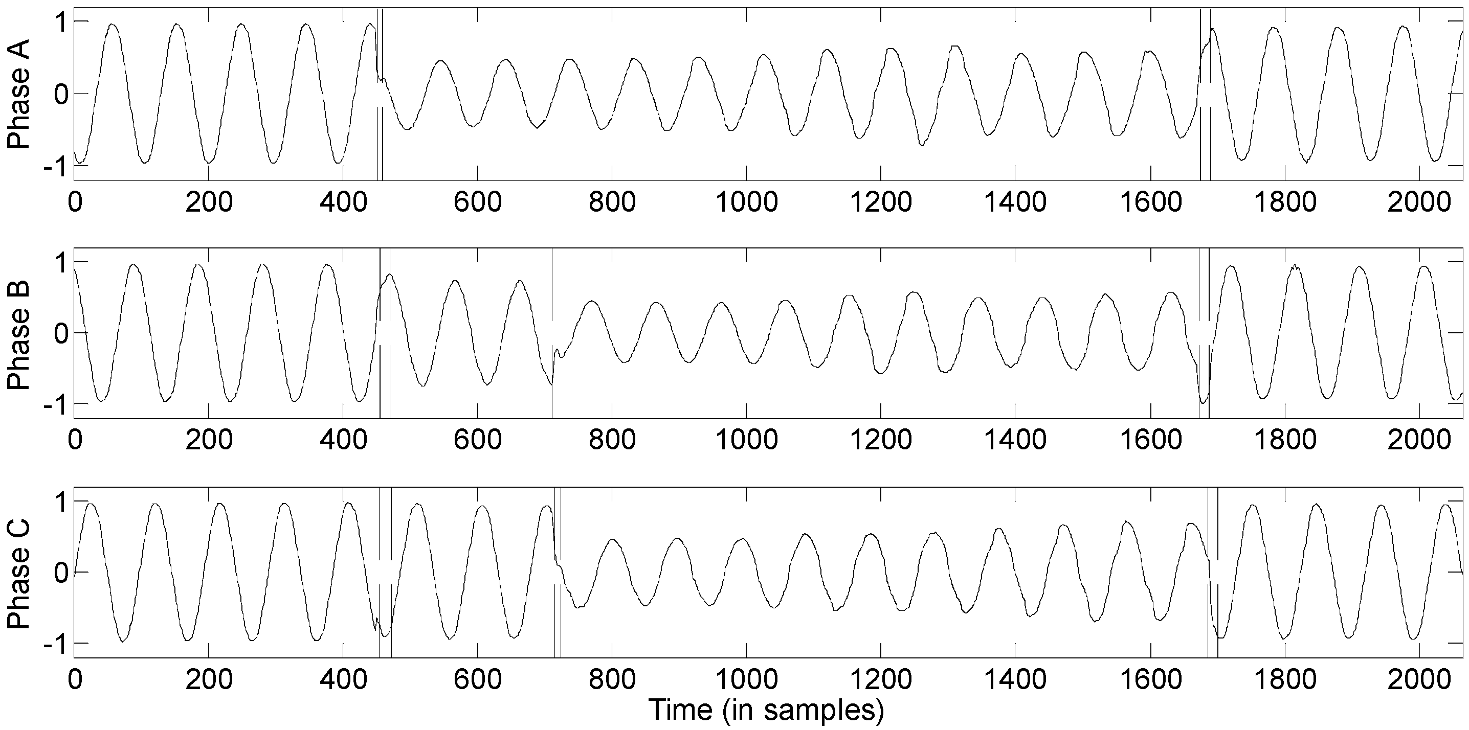
3.1. Segmentation Using Causal and Anti-Causal Methods

Figure 14 shows the CaC segmentation of the dip shown in Figure 13a. The CaC DPs are indicated in the graphs by the red line and the blue line, respectively. The values of the thresholds are very similar (H_c = 0.2869; H_ac = 0.2930) and their differences are not appreciated in the graphs. Finally, the segmentation is marked by the trigger points per transition, T_c (the vertical solid red line) and T_ac (the vertical solid blue line). Also shown in Figure 14 are the estimated time of the signal transitions per phase in the causal, S_c (the vertical dashed red line), and anti-causal, S_ac (the vertical dashed blue line), directions.

Figure 14. Causal and anti-causal segmentation of the dip.

Figure 14. Causal and anti-causal segmentation of the dip.

From the anti-causal results in several measurements, it was observed in the graphs that incrementing in one sample the S_ac value resulted in more accuracy in the detection start. This is because the anti-causal detection has a disadvantage here, as any transient due to the signal transition will occur after the transition so that the anti-causal detection will have a longer N than the causal detection. This adaptation of Equation (4) is considered in the following analysis.

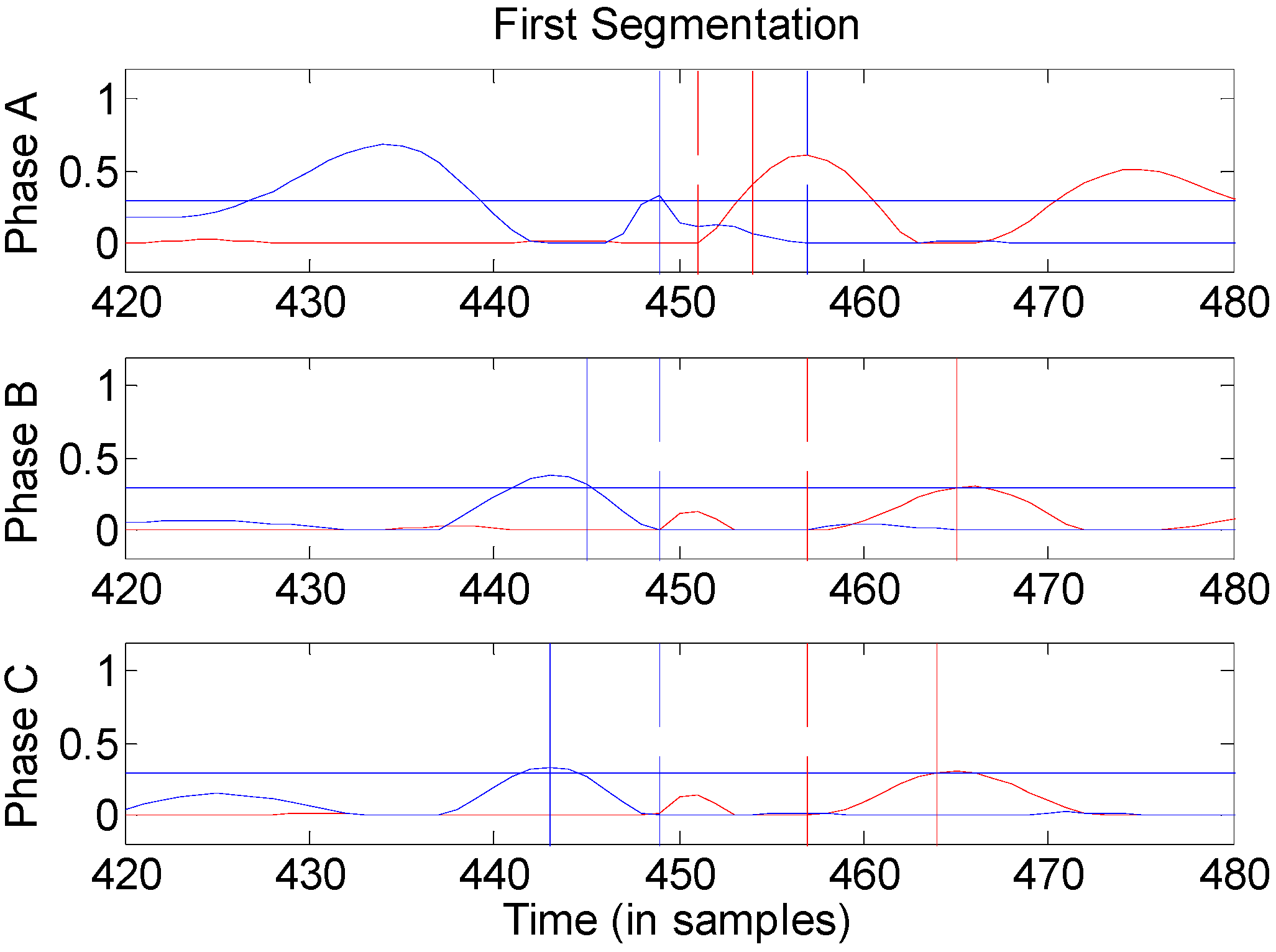
3.1.1. First Transition

Figure 15 shows the transitions that occurred per phase at the start of the dip. One can see that there is no overlap for the three phases (fast transitions) because the trigger time instant of the causal flag T_c (the vertical solid red line) is above the trigger time instant of the anti-causal flag T_ac (the vertical solid blue line). Also shown in Figure 15 are the start points of the transitions per phase in causal, S_c (the vertical dashed red line), and anti-causal, S_ac (the vertical dashed blue line), directions.

The points calculated for the transitions are shown in Table 1.

Figure 15. First segmentation: causal method shown in red (DP_c, H_c, T_c, S_c) and anti-causal method shown in blue (DP_ac, H_ac, T_ac, S_ac).

Figure 15. First segmentation: causal method shown in red (DP_c, H_c, T_c, S_c) and anti-causal method shown in blue (DP_ac, H_ac, T_ac, S_ac).

Table 1. Transition points for the first transition.

Phase	Tc (sample)	Tac (sample)	Nc (sample)	Nac (sample)	Sc (sample)	Sac (sample)
A	454	449	3	7	451	457
B	465	445	8	3	457	449
C	464	443	7	5	457	449

Table 1. Transition points for the first transition.

Phase	Tc (sample)	Tac (sample)	Nc (sample)	Nac (sample)	Sc (sample)	Sac (sample)
A	454	449	3	7	451	457
B	465	445	8	3	457	449
C	464	443	7	5	457	449

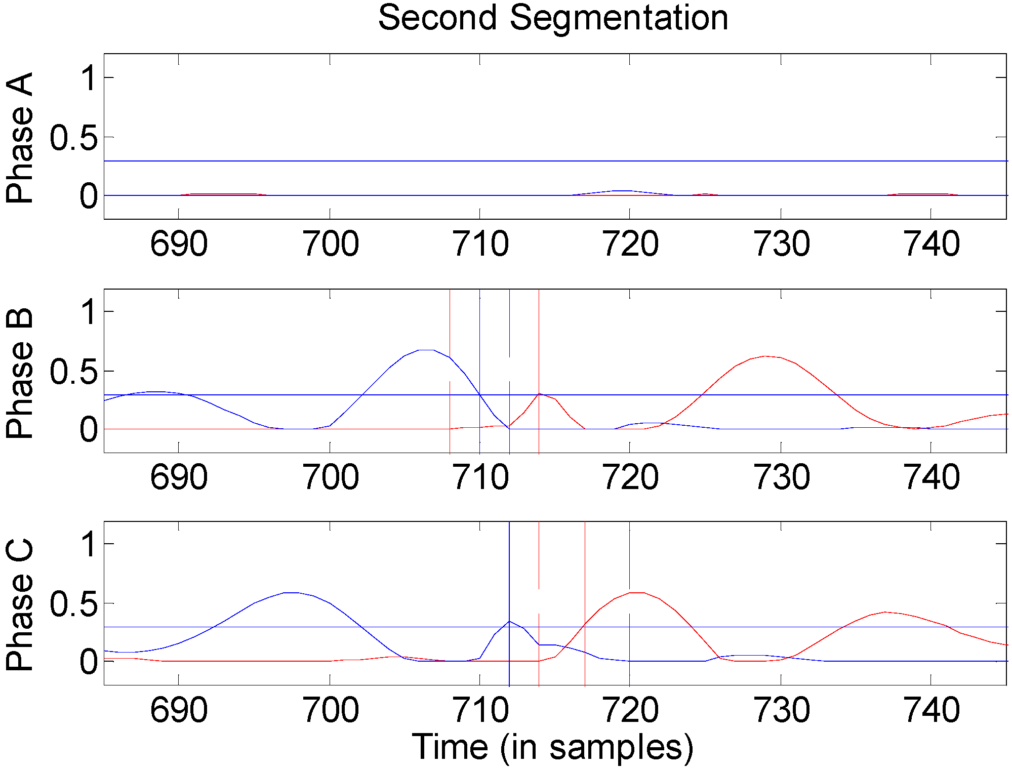
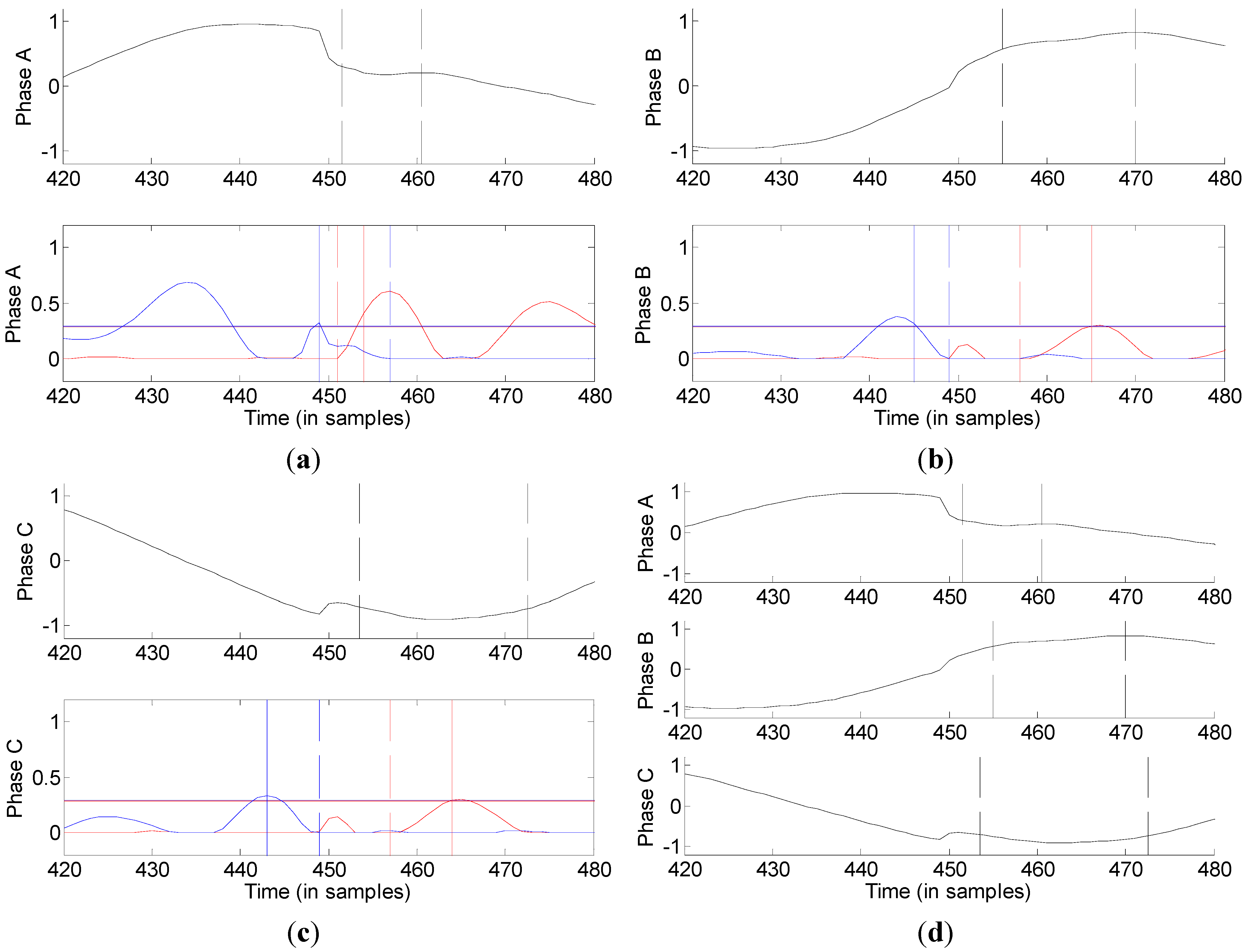
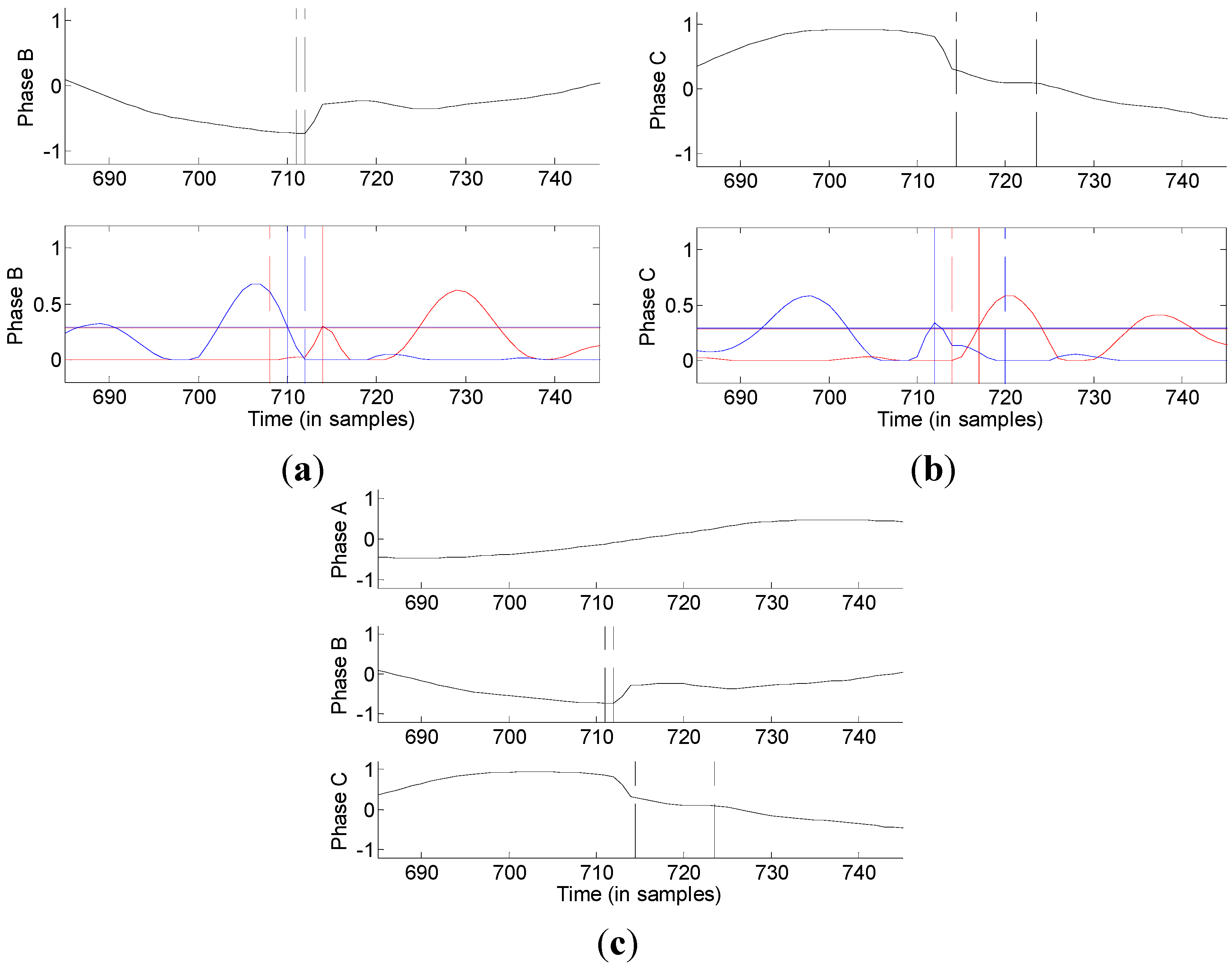
3.1.2. Second Transition

Figure 16 shows the transitions that occurred per phase at the second transition of the dip. One can see that there is a fast transition in phase B and phase C because the trigger time instant of the causal flag T_c (the vertical solid red line) is above the trigger time instant of the anti-causal flag T_ac (the vertical solid blue line). This segmentation indicates a fault inception between phase B and phase C; phase A is not involved. Figure 13 also shows the start points of the transitions per phase in causal, S_c (the vertical dashed red line), and anti-causal, S_ac (the vertical dashed blue line), directions.

Figure 16. Second segmentation: causal method shown in red (DP_c, H_c, T_c, S_c) and anti-causal method shown in blue (DP_ac, H_ac, T_ac, S_ac).

Figure 16. Second segmentation: causal method shown in red (DP_c, H_c, T_c, S_c) and anti-causal method shown in blue (DP_ac, H_ac, T_ac, S_ac).

The points calculated for the transitions are shown in Table 2.

Table 2. Transition points for the second transition.

Phase	Tc (sample)	Tac (sample)	Nc (sample)	Nac (sample)	Sc (sample)	Sac (sample)
A	-	-	-	-	-	-
B	714	710	6	1	708	712
C	717	712	3	7	714	720

Table 2. Transition points for the second transition.

Phase	Tc (sample)	Tac (sample)	Nc (sample)	Nac (sample)	Sc (sample)	Sac (sample)
A	-	-	-	-	-	-
B	714	710	6	1	708	712
C	717	712	3	7	714	720

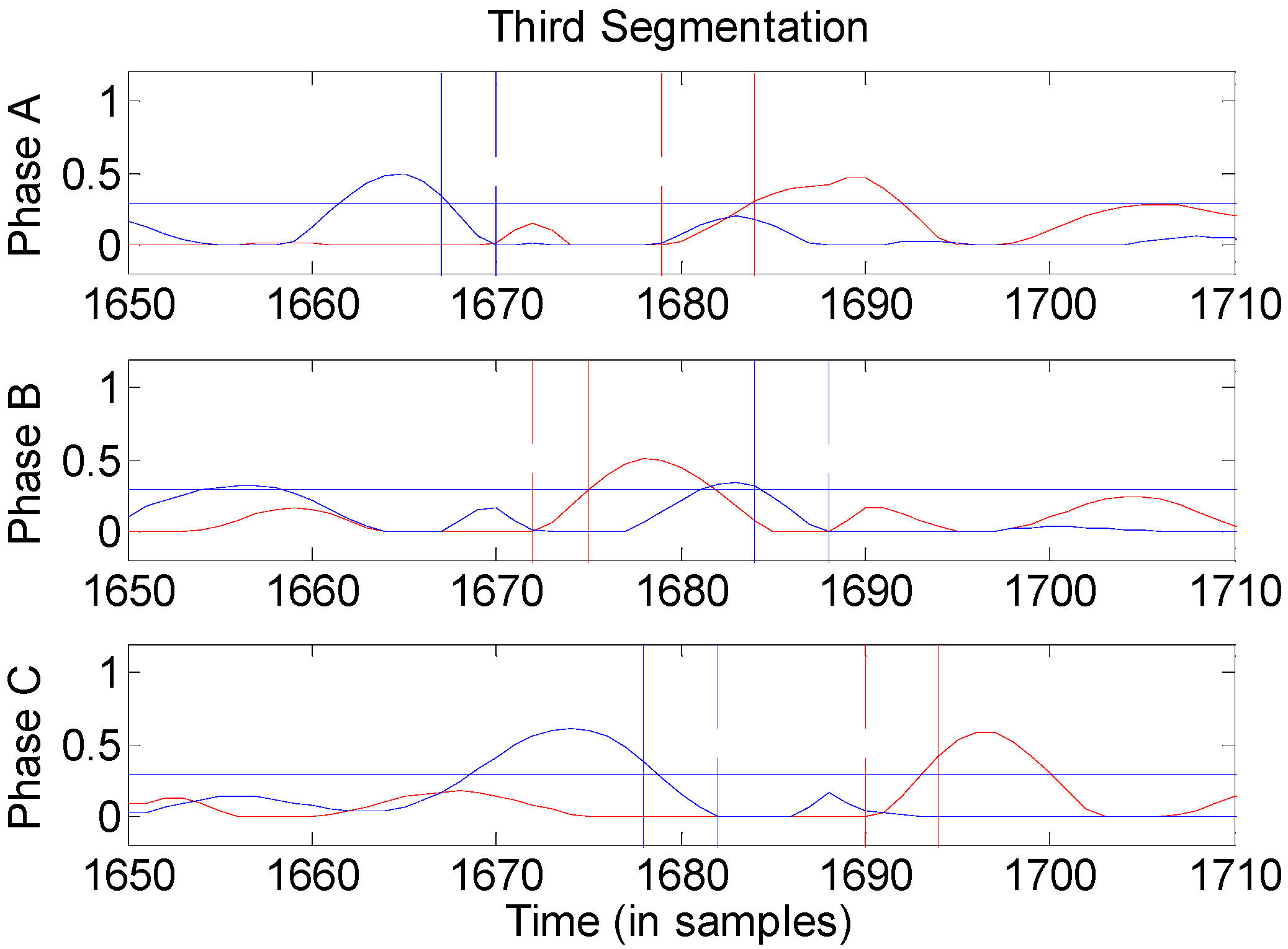
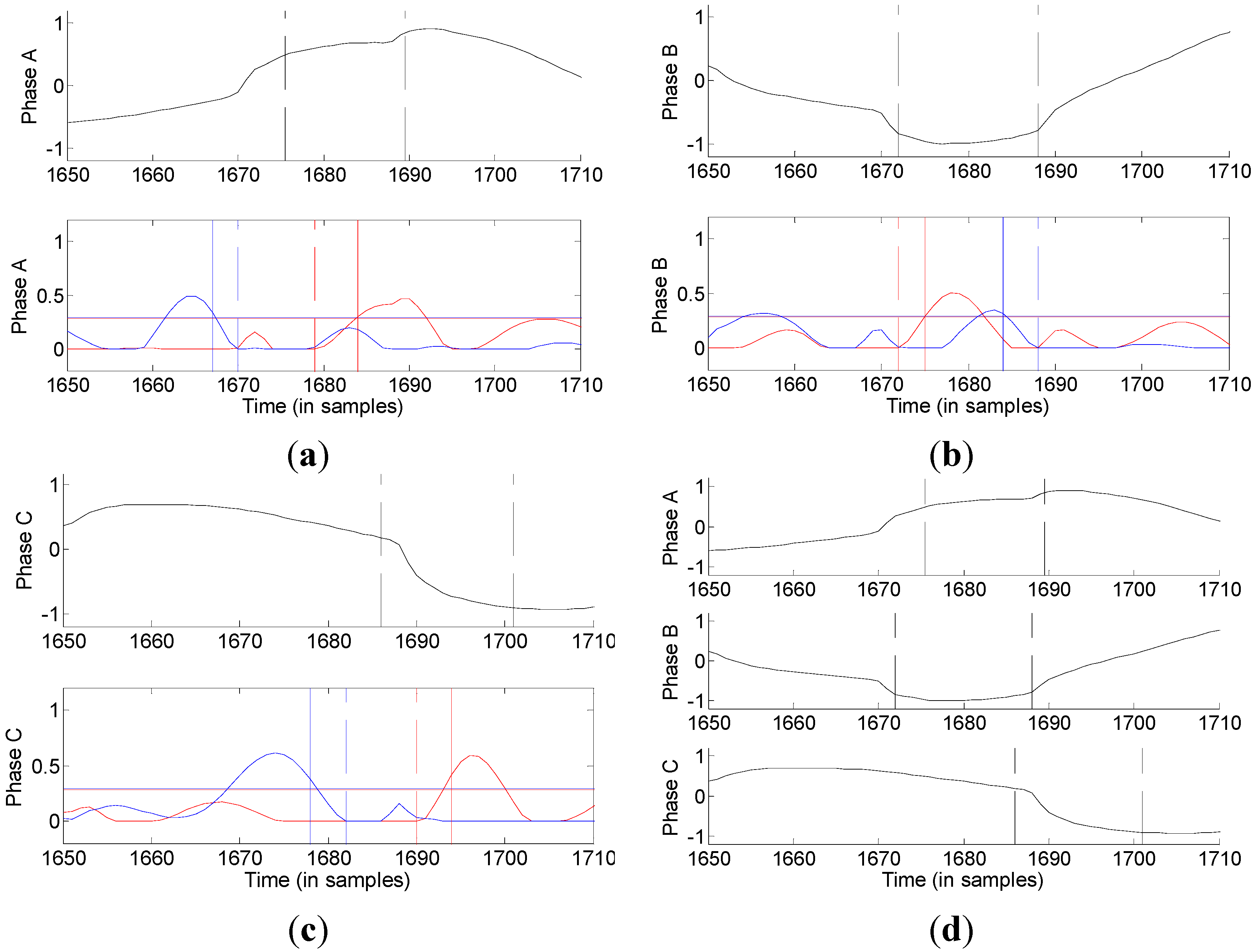
3.1.3. Third Transition

Figure 17 shows the transitions that occurred per phase at the recovery of the dip, causing transitions in the three phases. One can see that there is a fast transition in phase A and phase C and there is an overlap in phase B. In phase B, the trigger time instant of the causal flag T_c (the vertical solid red line) is below the trigger time instant of the anti-causal flag T_ac (the vertical solid blue line). Also shown in Figure 14 are the start points of the transitions per phase in causal, S_c (the vertical dashed red line), and anti-causal, S_ac (the vertical dashed blue line), directions.

Figure 17. Third segmentation: causal method shown in red (DP_c, H_c, T_c, S_c) and anti-causal method shown in blue (DP_ac, H_ac, T_ac, S_ac).

Figure 17. Third segmentation: causal method shown in red (DP_c, H_c, T_c, S_c) and anti-causal method shown in blue (DP_ac, H_ac, T_ac, S_ac).

The points calculated for the transitions are shown in Table 3.

Table 3. Transition points for the third transition.

Phase	Tc (sample)	Tac (sample)	Nc (sample)	Nac (sample)	Sc (sample)	Sac (sample)
A	1684	1667	5	2	1679	1670
B	1675	1684	3	3	1672	1688
C	1694	1678	4	3	1690	1682

Table 3. Transition points for the third transition.

Phase	Tc (sample)	Tac (sample)	Nc (sample)	Nac (sample)	Sc (sample)	Sac (sample)
A	1684	1667	5	2	1679	1670
B	1675	1684	3	3	1672	1688
C	1694	1678	4	3	1690	1682

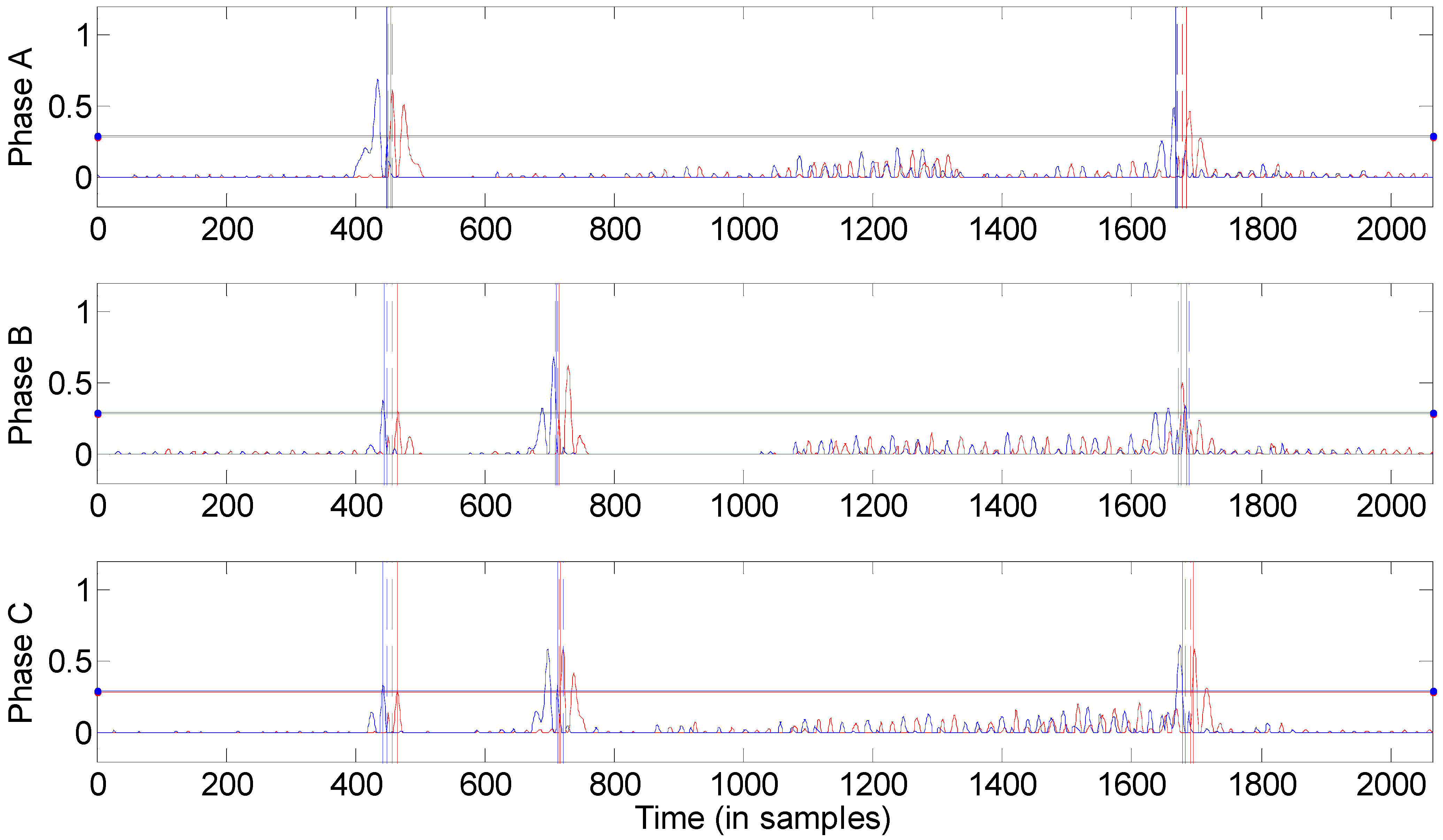
3.2. Estimate of the Signal Transitions Based on Causal and Anti-Causal Method

The following figures show the estimated start and end points of the actual signal transitions per phase, as well as the CaC segmentation, magnified, in areas around the transition segments.

3.2.1. First Transition

In the first transition of the dip, shown in Figure 18, there are fast transitions in the three phases, such that the estimated transitions have been calculated according to Equations (6) and (7).

Figure 18. Final segmentation and CaC segmentation for the first transition: (a) phase A; (b) phase B; (c) phase C; and (d) three-phase.

Figure 18. Final segmentation and CaC segmentation for the first transition: (a) phase A; (b) phase B; (c) phase C; and (d) three-phase.

3.2.2. Second Transition

In the second transition of the dip, shown in Figure 19, there are fast transitions in phase B and phase C. As with the previous case, the estimated transitions have been calculated according to Equations (6) and (7).

3.2.3. Third Transition

In the dip recovery, shown in Figure 20, there are fast transitions in phase A and C, so that the estimated transitions have been calculated according to Equations (6) and (7). In phase B there is a slow transition, and the estimated transition has been calculated according to Equation (5).

Figure 19. Final segmentation and CaC segmentation for the second transition: (a) phase B; (b) phase C; and (c) three-phase.

Figure 19. Final segmentation and CaC segmentation for the second transition: (a) phase B; (b) phase C; and (c) three-phase.

Figure 20. Final segmentation and CaC segmentation for the third transition: (a) phase A; (b) phase B; (c) phase C; and (d) three-phase.

Figure 20. Final segmentation and CaC segmentation for the third transition: (a) phase A; (b) phase B; (c) phase C; and (d) three-phase.

3.2.4. Final Three-Phase Segmentation of the Signal Transitions

The vertical lines in Figure 21 mark the beginning and the end of each estimated transition in the considered voltage dip. It can be observed that, for each phase, the proposed method consistently detects the actual signal transitions.

Figure 21. Final segmentation of the signal transitions in all three phases.

Figure 21. Final segmentation of the signal transitions in all three phases.

4. Conclusions

The present study provides a segmentation method that is useful for detecting transitions on recorded dips and accurately determining the times at which they occur. The proposed method combines CUSUM as a statistical estimator with joint CaC segmentation. The proposed method accurately detects the transition segments for the three-phase dips. The method overcomes the detection-delay problem of conventional methods by combining both forward (causal) and backward (anti-causal) segmentation to estimate the location in time of the transition segments. In addition, the method improves the detection-delay problem inherent to the analysis windows of conventional methods by including a counter that determines the time elapsed between the start of the transition and the detection instant. Moreover, a method to determine the threshold setting for the detection index, configured with a high probability of detection and a low false alarm rate, has been proposed. Experimental results show very good performance for measured voltage dips in a real power system. Furthermore, analyzing both forward and backward-sliding windows, the method is able to distinguish slow and fast transitions throughout the recorded dip. Further research is needed to study the relationship of the dip’s segmentation with its start and its recovery with the proposed method, with the final purpose of looking for a relationship with other classification methods such as symmetrical components classification or the ABC classification. The overall aim of this work is to design robust classifiers that provide an easy way to characterize events that occur in the power system with high accuracy and, consequently, to determine the origin of those events.

References

1. Dugan, R.C.; McGranaghan, M.F.; Santoso, S.; Beaty, H.W. Electrical Power Systems Quality, 3rd ed.; McGraw Hill Professional: New York, NY, USA, 2012. [Google Scholar]
2. Moreno-Muñoz, A. Power Quality: Mitigation Technologies in a Distributed Environment; Springer Science & Business Media: New York, NY, USA, 2007. [Google Scholar]
3. Mozina, C.J. Interconnection protection of IPP generators at commercial/industrial facilities. IEEE Trans. Ind. Appl. 2001, 37, 681–688. [Google Scholar] [CrossRef]
4. Moreno-Munoz, A.; de-la-Rosa, J.J.G.; Lopez-Rodriguez, M.A.; Flores-Arias, J.M.; Bellido-Outerino, F.J.; Ruiz-de-Adana, M. Improvement of power quality using distributed generation. Int. J. Electr. Power Energy Syst. 2010, 32, 1069–1076. [Google Scholar] [CrossRef]
5. Moreno-Munoz, A.; Flores-Arias, J.; Gil-de-Castro, A.; de-la-Rosa, J.J.G. Power quality for energy efficient buildings. In Proceedings of the 2009 International Conference on Clean Electrical Power, Capri Capri, Italy, 9–11 June 2009; IEEE: Piscataway, NJ, USA, 2009; pp. 191–195. [Google Scholar]
6. Ribeiro, P.F.; Duque, C.A.; Ribeiro, P.M.; Cerqueira, A.S. Power Systems Signal Processing for Smart Grids; Wiley: Hoboken, NJ, USA, 2013. [Google Scholar]
7. Bollen, M.; Gu, I.; Santoso, S.; Mcgranaghan, M.; Crossley, P.; Ribeiro, M.; Ribeiro, P. Bridging the gap between signal and power. IEEE Signal Process. Mag. 2009, 26, 12–31. [Google Scholar] [CrossRef]
8. Gu, I.Y.H.; Ernberg, N.; Styvaktakis, E.; Bollen, M.H.J. A Statistical-Based Sequential Method for Fast Online Detection of Fault-Induced Voltage Dips. IEEE Trans. Power Deliv. 2004, 19, 497–504. [Google Scholar] [CrossRef]
9. De Apráiz, M.; Barros, J.; Diego, R.I. A real-time method for time-frequency detection of transient disturbances in voltage supply systems. Electr. Power Syst. Res. 2014, 108, 103–112. [Google Scholar] [CrossRef]
10. Huang, N.; Zhang, S.; Cai, G.; Xu, D. Power Quality Disturbances Recognition Based on a Multiresolution Generalized S-Transform and a PSO-Improved Decision Tree. Energies 2015, 8, 549–572. [Google Scholar] [CrossRef]
11. Le, C.D.; Gu, I.Y.H.; Bollen, M.H.J. Joint causal and anti-causal segmentation and location of transitions in power disturbances. In Proceedings of the 2010 IEEE Power and Energy Society General Meeting, Minneapolis, MN, USA, 25–29 July 2010; IEEE: Piscataway, NJ, USA, 2010; pp. 1–6. [Google Scholar]
12. Bollen, M.H.; Gu, I. Signal Processing of Power Quality Disturbances; John Wiley & Sons: Hoboken, NJ, USA, 2006. [Google Scholar]
13. Gustafsson, F. Adaptive Filtering and Change Detection; Wiley: Hoboken, NJ, USA, 2000. [Google Scholar]
14. Mohanty, S.R.; Pradhan, A.K.; Routray, A. A Cumulative Sum-Based Fault Detector for Power System Relaying Application. IEEE Trans. Power Deliv. 2008, 23, 79–86. [Google Scholar] [CrossRef]
15. Noori, M.R.; Jamali, S.; Shahrtash, S.M. Security assessment for a cumulative sum-based fault detector in transmission lines. In Proceedings of the 2011 10th International Conference on Environment and Electrical Engineering (EEEIC), Rome, Italy, 8–11 May 2011; IEEE: Piscataway, NJ, USA, 2011; pp. 1–5. [Google Scholar]
16. Montgomery, D.C. Introduction to Statistical Quality Control; Wiley: Hoboken, NJ, USA, 2008. [Google Scholar]
17. Basseville, M.; Nikiforov, I.V. Detection of Abrupt Changes: Theory and Application; Prentice Hall: Upper Saddle River, NJ, USA, 1993. [Google Scholar]