Wind Resource Mapping Using Landscape Roughness and Spatial Interpolation Methods

Abstract

Energy saving, reduction of greenhouse gasses and increased use of renewables are key policies to achieve the European 2020 targets. In particular, distributed renewable energy sources, integrated with spatial planning, require novel methods to optimise supply and demand. In contrast with large scale wind turbines, small and medium wind turbines (SMWTs) have a less extensive impact on the use of space and the power system, nevertheless, a significant spatial footprint is still present and the need for good spatial planning is a necessity. To optimise the location of SMWTs, detailed knowledge of the spatial distribution of the average wind speed is essential, hence, in this article, wind measurements and roughness maps were used to create a reliable annual mean wind speed map of Flanders at 10 m above the Earth’s surface. Via roughness transformation, the surface wind speed measurements were converted into meso- and macroscale wind data. The data were further processed by using seven different spatial interpolation methods in order to develop regional wind resource maps. Based on statistical analysis, it was found that the transformation into mesoscale wind, in combination with Simple Kriging, was the most adequate method to create reliable maps for decision-making on optimal production sites for SMWTs in Flanders (Belgium).

1. Introduction

Next to energy savings and reduction of emissions, an increased share of renewables in the European energy mix is a key priority of the Energy Union [1]. With a target of 20% by 2020 and 27% by 2030, Europe has set ambitious goals for renewable energy, requiring a broad mix of clean technologies, both large and small scale, to take a share.

Over time, technical research and innovation projects on distributed renewable energy sources (DRES)—such as small and medium wind turbines (SMWTs)—have been a primary focal area of interest. However, wind energy generation is difficult to manage because of the irregular nature of wind flows. Further, the current transition in energy demand and supply also encompasses many aspects, such as the resource availability evaluation, the compliance with environmental and legal constraints, and many more technical aspects. In this complex context, understanding the spatial distribution of the long-term average wind speed is essential for decision-making, particularly in regards to the siting of wind turbines. Hence, the current transition in distributed energy demand and supply prompts a new area of research: spatial energy planning. Further, by combining technical and spatial wind research and integrating it with regulatory, economic and social constraints, a new interdisciplinary research and innovation area is unfolded with a high valorisation potential for energy prosumers on a local scale.

Understanding the spatial distribution of the long-term mean wind speed is essential for decision-making, particularly in regards to the siting of wind turbines. However, there is often a lack of measurements to enable accurate wind speed mapping. Despite the long evolution of wind mapping and method development for assessing wind as a resource, along with increasing computational capabilities, a single general method for creating predicative wind maps does not exist. Indeed, a reliable approach depends on a number of factors that are context-related: the size of the analysed area, the required resolution of the results, the climatic and topographical characteristics of the analysed area, the density of the available meteorological measurements, etc. [2].

In regions like Flanders (Belgium), an area of 13,522 km² with ca. 6.4 million inhabitants and a high potential in terms of wind power generation, efficient energy planning based on renewables is a complex task. In fact, the region is characterised by a composite topography, a compound of land covers and dispersed buildings. The open space is no longer a monofunctional agricultural production area but, rather, a complex structure of fragments with varying densities and functions [3]. Marked by a dense matrix of meteorological stations, this region is challenging for identifying optimal SMWT locations.

Next to meteorological data, basic wind speed measurements are equally available at various heights, covering the entire Flemish region. As shown in Figure 1, a primary wind study for Belgium was performed in 1984 by Hirsch. Although an interesting effort, it provides insufficient insight in local wind availabilities to enable detailed siting for SMWTs. In 2014, a roughness map was generated for the Flemish region by converting land cover categories into sequences of roughness length [4].

Figure 1. Annual mean wind speed map of Belgium [5].

Figure 1. Annual mean wind speed map of Belgium [5].

This article starts from the results of the latter study and develops a detailed low-height wind speed map, providing a useful tool for the identification of optimal locations for SMWTs in Flanders. The research aim is not to develop new methodologies, although some are described in Section 3, but to analyse data by applying already existing methods and producing an updated wind map, which is valuable for deployment of micro-wind energy.

Another advantage of the proposed methodology is that it uses open source data and software. Compared to the method we propose here, more sophisticated models (i.e., Wasp or windPRO) and data assimilation techniques have been developed in literature, but they are not affordable for use by small municipalities.

In Section 2, the wind speed measurements for Flanders and the roughness map are presented, providing the geo-database used in this study. Section 3 describes two types of exposure corrections and introduces the seven interpolation methods assessed in this study. The results are discussed and mapped in Section 4, and presents the conclusions of the selected methodologies for wind resource mapping. In order to demonstrate how the Annual Energy Production (AEP) can be calculated for a specific small or medium wind turbine, an AEP map is created in Section 5 for a 10 kW 3-blade, upwind, horizontal axis wind turbine. A Rayleigh distribution, which is identical to a Weibull distribution with shape factor 2, is used as the reference wind speed frequency distribution.

2. Data collection

2.1. Wind speed Measurements

This work is based on the wind data recorded in a number of Flemish meteorological stations spread over the region. The study used recent observed data since both the wind climate and the environment have changed in the past decades. The collected data, location of meteorological stations, relative recording dates and local wind speed measurements used in this study are summarised in Table 1. The geographic location of the meteorological stations is visualised in Figure 2.

Figure 2. Location of the measurement stations used.

Figure 2. Location of the measurement stations used.

Daily wind speed observations obtained from the National Climatic Data Center (NCDC) of the US National Oceanic and Atmospheric Administration (NOAA) [6] were collected for all available stations in Belgium, with the addition of some frontier mast data from the Netherlands and France. All stations are equipped with an anemometer at the height of 10 m, hence, the observed wind speed is the so-called “surface wind speed”, which is further averaged over a calendar year so as to rule out seasonal bias. Data validation is performed by using the more accurate and precise dataset created by the Royal Meteorological Institute (RMI), which refers to a smaller group of 18 stations selected from the original number.

The data from NCDC include the average wind speed at 10 m for France, the Netherlands and Belgium. The data are validated through comparison with the corresponding dataset from RMI (for Flanders). Apart from being rounded to one decimal place, both sets are identical, therefore the extensive open-source database of NCDC is selected for producing regional wind maps in this study.

Since recent studies suggest that climate change is affecting the prevailing wind profiles, 40-year-old observations are considered inadequate for future wind modelling [7]. Likewise, the landscape in Flanders has significantly changed over the past decades due to the development of built-up areas [8]. Therefore, meteorological stations with recent wind data (2010–2014) were selected and the annual mean wind speed was calculated based on five years of measurements, with the exception of Sint-Katelijne-Waver (only 2013–2014 available). Even with a reduced number of recent observations as recorded in Table 1, it is observed that there is a decreasing trend of the annual mean wind speed over the last five years.

Table 1. Summary of the measurement stations (height 10 m). The recent data is (2010–2014) indicated in bold letter type [6].

Station	Roughness [m]	Latitude [°]	Longitude [°]	Begin Date	End Date	Mean Wind Speed [m/s]	Mean Wind Speed (2010–2014) [m/s]
Beauvechain	0.03	50.758	4.768	1/01/1973	42.004	3.88	3.70
Beitem	0.469	50.900	3.116	1/02/2008	42.035	3.69	3.67
Brasschaat	0.14	51.333	4.500	1/02/1973	31/01/2006	3.26
Brussels NATL	0.037	50.902	4.485	1/01/1973	31/12/2014	3.99	3.62
Brussels South	0.2	50.459	4.453	1/01/1973	31/12/2014	3.96	4.00
Buzenol	0.6	49.616	5.583	26/10/2009	25/10/2014	2.76	2.74
Casteau/Heli	0.8	50.500	3.980	1/01/2011	31/12/2014	2.18
Chievres	0.1	50.575	3.831	1/01/1973	31/12/2014	3.73	3.75
Deurne	0.896	51.189	4.460	1/01/1973	31/12/2014	3.55	3.58
Diepenbeek	0.08	50.916	5.450	1/01/2010	31/12/2014	2.92	2.92
Dourbes	0.6	50.100	4.600	1/01/2010	31/12/2014	2.52	2.52
Elsenborn	0.6	50.466	6.183	1/01/1987	31/12/2014	3.11	3.12
Ernage	0.1	50.583	4.683	1/01/2008	31/12/2014	4.06	4.04
Florennes	0.15	50.243	4.645	1/01/1973	31/12/2014	3.75	3.69
Genk/Zwartberg	0.676	51.012	5.522	7/01/1973	6/01/2004	3.60
Gent/Industrie	0.021	51.187	3.799	1/01/1985	31/12/2014	3.31	3.32
Humain	0.4	50.200	5.250	1/03/2010	28/02/2015	3.69	3.66
Kleine Brogel	0.054	51.168	5.470	1/01/1973	31/12/2014	3.01	3.01
Koksijde	0.06	51.090	2.652	1/01/1973	31/12/2014	4.68	4.57
Liege	0.15	50.637	5.443	1/01/1973	31/12/2014	4.07	4.11
Melle	0.2	50.983	3.816	1/01/2010	31/12/2014	3.42	3.42
Mont-Rigi	0.2	50.516	6.066	16/01/2008	15/01/2015	3.83	3.74
Oostende	0.64	51.198	2.862	1/01/1973	31/12/2014	5.22	4.75
Oostende (Pier)	0.98	51.235	2.914	1/01/1973	31/12/2005	6.91
Retie	0.118	51.216	5.033	26/10/2009	25/10/2014	2.64	2.63
Saint Hubert Mil	0.2	50.035	5.404	1/01/1973	31/12/2014	3.88	3.29
Schffen	0.03	51.000	5.066	2/01/1973	1/01/2015	3.93	3.21
Semmerzake	0.231	50.933	3.666	1/01/1973	31/12/2014	3.70	3.26
Sinsin	0.3	50.266	5.250	20/09/1984	19/09/1995	3.49
Sint Katelijne-waver	0.278	51.070	4.535	1/10/2012	30/09/2014	3.02	3.05
Sint Truiden	0.03	50.791	5.201	1/01/1973	31/12/1991	3.62
Spa/La Sauveniere	0.1	50.483	5.916	1/01/1974	31/12/2014	3.87	3.74
Uccle	0.621	50.800	4.350	1/01/1973	31/12/2014	3.48	3.44
Zeebrugge	0.001	51.350	3.200	26/10/2009	25/10/2014	6.05	6.02
Dunkerque	0.01	51.050	2.333	2/01/1973	1/01/2015	6.20	5.26
Lesquin	0.1	50.561	3.089	1/01/1973	31/12/2014	4.37	4.09
Eindhoven	0.1	51.450	5.374	1/01/1973	31/12/2014	3.94	3.64
Ell AWS	0.15	51.200	5.766	1/01/2002	31/12/2014	3.53	3.46
Gilze Rijen	0.05	51.567	4.931	1/01/1973	31/12/2014	3.81	3.53
Maastricht	0.05	50.911	5.770	1/01/1973	31/12/2014	4.25	4.06
Vlissingen	0.25	51.450	3.600	1/01/1973	31/12/2014	6.07	6.10
Westdorpe	0.25	51.233	3.866	1/01/1995	31/12/2014	4.02	4.00
Woensdrecht	0.3	51.449	4.342	1/01/1996	31/12/2014	3.45	3.48

Table 1. Summary of the measurement stations (height 10 m). The recent data is (2010–2014) indicated in bold letter type [6].

Station	Roughness [m]	Latitude [°]	Longitude [°]	Begin Date	End Date	Mean Wind Speed [m/s]	Mean Wind Speed (2010–2014) [m/s]
Beauvechain	0.03	50.758	4.768	1/01/1973	42.004	3.88	3.70
Beitem	0.469	50.900	3.116	1/02/2008	42.035	3.69	3.67
Brasschaat	0.14	51.333	4.500	1/02/1973	31/01/2006	3.26
Brussels NATL	0.037	50.902	4.485	1/01/1973	31/12/2014	3.99	3.62
Brussels South	0.2	50.459	4.453	1/01/1973	31/12/2014	3.96	4.00
Buzenol	0.6	49.616	5.583	26/10/2009	25/10/2014	2.76	2.74
Casteau/Heli	0.8	50.500	3.980	1/01/2011	31/12/2014	2.18
Chievres	0.1	50.575	3.831	1/01/1973	31/12/2014	3.73	3.75
Deurne	0.896	51.189	4.460	1/01/1973	31/12/2014	3.55	3.58
Diepenbeek	0.08	50.916	5.450	1/01/2010	31/12/2014	2.92	2.92
Dourbes	0.6	50.100	4.600	1/01/2010	31/12/2014	2.52	2.52
Elsenborn	0.6	50.466	6.183	1/01/1987	31/12/2014	3.11	3.12
Ernage	0.1	50.583	4.683	1/01/2008	31/12/2014	4.06	4.04
Florennes	0.15	50.243	4.645	1/01/1973	31/12/2014	3.75	3.69
Genk/Zwartberg	0.676	51.012	5.522	7/01/1973	6/01/2004	3.60
Gent/Industrie	0.021	51.187	3.799	1/01/1985	31/12/2014	3.31	3.32
Humain	0.4	50.200	5.250	1/03/2010	28/02/2015	3.69	3.66
Kleine Brogel	0.054	51.168	5.470	1/01/1973	31/12/2014	3.01	3.01
Koksijde	0.06	51.090	2.652	1/01/1973	31/12/2014	4.68	4.57
Liege	0.15	50.637	5.443	1/01/1973	31/12/2014	4.07	4.11
Melle	0.2	50.983	3.816	1/01/2010	31/12/2014	3.42	3.42
Mont-Rigi	0.2	50.516	6.066	16/01/2008	15/01/2015	3.83	3.74
Oostende	0.64	51.198	2.862	1/01/1973	31/12/2014	5.22	4.75
Oostende (Pier)	0.98	51.235	2.914	1/01/1973	31/12/2005	6.91
Retie	0.118	51.216	5.033	26/10/2009	25/10/2014	2.64	2.63
Saint Hubert Mil	0.2	50.035	5.404	1/01/1973	31/12/2014	3.88	3.29
Schffen	0.03	51.000	5.066	2/01/1973	1/01/2015	3.93	3.21
Semmerzake	0.231	50.933	3.666	1/01/1973	31/12/2014	3.70	3.26
Sinsin	0.3	50.266	5.250	20/09/1984	19/09/1995	3.49
Sint Katelijne-waver	0.278	51.070	4.535	1/10/2012	30/09/2014	3.02	3.05
Sint Truiden	0.03	50.791	5.201	1/01/1973	31/12/1991	3.62
Spa/La Sauveniere	0.1	50.483	5.916	1/01/1974	31/12/2014	3.87	3.74
Uccle	0.621	50.800	4.350	1/01/1973	31/12/2014	3.48	3.44
Zeebrugge	0.001	51.350	3.200	26/10/2009	25/10/2014	6.05	6.02
Dunkerque	0.01	51.050	2.333	2/01/1973	1/01/2015	6.20	5.26
Lesquin	0.1	50.561	3.089	1/01/1973	31/12/2014	4.37	4.09
Eindhoven	0.1	51.450	5.374	1/01/1973	31/12/2014	3.94	3.64
Ell AWS	0.15	51.200	5.766	1/01/2002	31/12/2014	3.53	3.46
Gilze Rijen	0.05	51.567	4.931	1/01/1973	31/12/2014	3.81	3.53
Maastricht	0.05	50.911	5.770	1/01/1973	31/12/2014	4.25	4.06
Vlissingen	0.25	51.450	3.600	1/01/1973	31/12/2014	6.07	6.10
Westdorpe	0.25	51.233	3.866	1/01/1995	31/12/2014	4.02	4.00
Woensdrecht	0.3	51.449	4.342	1/01/1996	31/12/2014	3.45	3.48

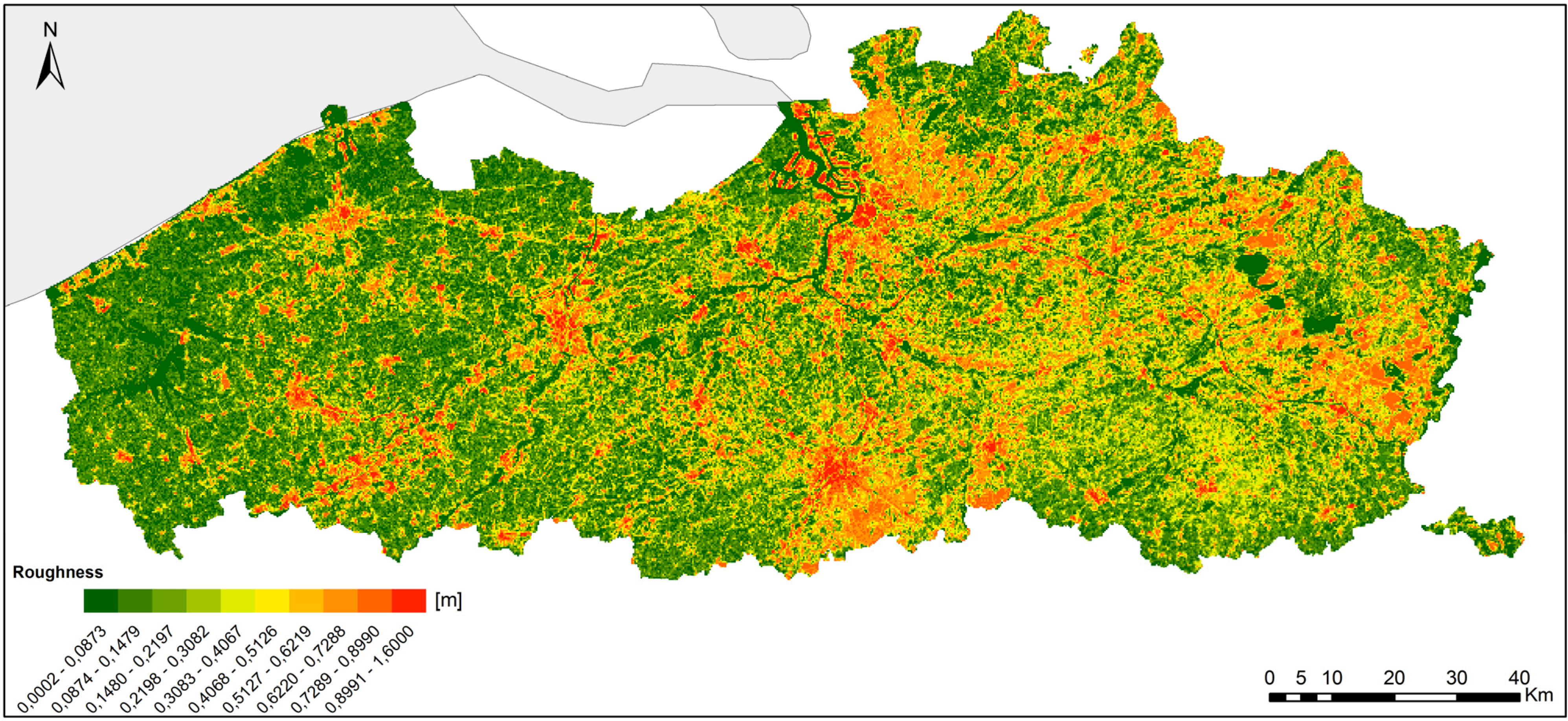
2.1.1. Roughness Map Flanders

To account for the different surfaces in Flanders, a roughness map, developed in 2014 [4], was used. The map uses the roughness length of a land mark as indicator, defined by [9]. In this case, a resolution of 250 by 250 meters is presented (see Figure 3).

Figure 3. Roughness map of Flanders [4].

Figure 3. Roughness map of Flanders [4].

Whilst the roughness length (z₀) is not a physical length, it can be considered as a length-scale representing the roughness of the surface: for example, forests have a much larger roughness length than open sea areas. At a low height above the ground, or the surface layer, the roughness of a terrain affects the turbulence intensity as well as the vertical wind pattern and, by consequence, the wind speed. The roughness map was constructed by the Flemish Institute for Technological Research (VITO) based on the CoORdination of INformation on the Environment (CORINE) Land Cover 2000 data set [9]. In this project, the National Geographic Institute (NGI) constructed the national land cover map using high resolution (Landsat Thematic Mapper) satellite images [10]. The detailed map enables correction of the observations for local sheltering and topography.

3. Methodology

In this section, the statistical interpretation process of the wind time series is explained. In detail, the section describes how seven different interpolation methods are tested and assessed in order to select the most performant way to generate a wind resource map of Flanders.

3.1. The PBL Two Layer Model

Over the last two decades, several studies have been carried out with the aim of creating an adequate statistical model for describing the wind speed frequency distribution. One of the more recent studies developed for the Netherlands [11] used the Planetary Boundary Layer (PBL) two-layer model. This two-layer transformation model from Wieringa [12] was further developed by Verkaik [13,14,15,16,17] and more recently by Wever and Groen [18]. The methodology is generally accepted and recommended [19,20,21,22], however, the report admits to not having explored the potential benefits of using Kriging (see Section 3.2.2), as detailed in Section 3.3 of [11].

In the research carried out by Wieringa in the 70s and 80s [12,23], wind speed variations on a resolution of 250 by 250 meters are caused mainly by differences in atmospheric stability and surface roughness. At a certain so-called blending height [12] these variations become negligible compared to the average speed, yielding a spatially homogeneous dataset suitable for interpolation. A roughness correction is applied to the observations by using the measured surface wind speed to calculate the regional wind speed that is representative for a larger area by using the roughness length of the meteorological station. After completion of the spatial interpolation, the regional winds are used to calculate the wind speed at 10 m by using the inverse roughness correction and by using the roughness map of Flanders [24]. Finally, according to this methodology, two different regional wind speeds are used for interpolation. This “roughness blending height” is set to be z_b = 60 m [23]. The macrowind speed is measured at the top of the PBL.

3.1.1. Mesowind

At the blending height z_b defined above, land covers and local obstacles have a minimal influence on the wind speed. This height is set to be z_b = 60 m. The observed surface wind speed, U_s, can be used to calculate the mesowind speed, U_meso, by assuming a logarithmic wind profile [24]:

$$U_{\text{meso}}=U_{\text{s}} \frac{\ln (\frac{z_b}{z_{0s}})}{\ln (\frac{z_s}{z_{0s}})}$$

(1)

with z_0s as the roughness length at the meteorological station site and z_s as the anemometer height, equal to 10 m for all stations in this study. For all stations in Flanders, Wallonia, France and the Netherlands, the roughness length z_0s was estimated from a terrain description and by using data based on satellite images of the sites [25].

It is shown that the mesoscale wind climate is spatially more homogeneous than the surface wind [11], hence, it is better suited for interpolation. The interpolated U_meso values in Flanders are then reconverted to the surface wind speed at 10 m, U_10m, by using [24]:

$$U_{\text{1}0\text{m}}=U_{\text{meso}} \frac{\ln (\frac{10}{z_0})}{\ln (\frac{z_b}{z_0})}$$

(2)

with z₀ as the roughness length at each 250 m pixel from the roughness map.

3.1.2. Macrowind

The use of macrowind for interpolation purposes is described by Wieringa and is further used to create a gridded wind speed map of the Netherlands [11]. In this method, two layers are defined. In the lower layer, the surface layer, Monin-Obukhov theory is used [26,27]. In this theory, the logarithmic wind speed profile is used to express the increase in wind speed U in the lower layer [28]:

$$U=\frac{u^{*}}{\text{κ}} \ln (\frac{z}{z_{0s}})$$

(3)

by using the local roughness length at the site z_0s and the Von Kármán constant κ = 0.4 [29,30]. u^* is the friction velocity and is constant with height over homogeneous terrain, which makes it possible to calculate u^* at the meteorological stations.

Geostrophic drag relations apply in the second higher layer, the planetary boundary layer (PBL). In the PBL, the wind speed increases further and in addition the wind direction veers (turns clockwise) such that a second wind speed component perpendicular to the surface wind speed (V_macro) is formed [31]:

$$\frac{\text{κ}(U-U_{\text{macro}})}{u^{*}}=\left[\ln \left(\frac{z f}{u^{*}}\right)+A\right]$$

(4)

$$V_{\text{macro}}=B \frac{u^{*}}{\text{κ}}$$

(5)

with the Coriolis parameter f = 1.129 × 10⁻⁴ at 51°N [32]. The stability parameters A and B are equal to 1.9 and 4.5 respectively, as is generally accepted in literature [17] when assuming neutral stability [33]. The vertical extrapolation methods rely on the neutral stability assumption; although neutral conditions characterised by log-profiles are common in general, stable and unstable conditions with non-log vertical profiles occur often as well [34].

The wind at this PBL is called the macrowind, S_macro, and varies on a larger scale than the mesowind [12]. The macrowind S_macro consists of two components: U_macro is parallel to the surface wind and V_macro is perpendicular to U_macro. Matching the two layers at the mesolevel according to Equations (3) and (4) leads to [17]:

$$U_{\text{macro}}=\frac{u^{*}}{\text{κ}}\left[\ln \left(\frac{u^{*}}{f z_{0s}}\right)-A\right]$$

(6)

The PBL ranges from a few hundred meters to a few kilometres above the surface of the Earth [35], the height of the top of the PBL is given by [17]:

$$h=\frac{u^{*}}{f{e}^A}$$

(7)

Both components U_macro and V_macro and the root of the squared sum (macrowind speed, S_macro) are interpolated by using Simple Kriging separately onto the 250 m resolution grid of the regional surface roughness map. Such obtained S_macro values are cross-checked with the values calculated from the interpolated U_macro and V_macro, yielding differences that are negligibly small.

After spatial interpolation of the S_macro values at different location points, S_macro is used to calculate the surface wind speed at these locations, by using the inverse process. First the friction velocity u^* needs to be calculated, by using Equations (5) and (6), in order to calculate the surface wind speed U_10m with Equation (3) using z₀ instead of z_0s (see Figure 4b).

3.2. Spatial Interpolation Methods

In order to obtain an accurate picture of the Flemish wind potential, in addition to the roughness map and meteorological observations, the wind speed was estimated at un-recorded sites via spatial interpolation of the measured data.

Various interpolation techniques are available, of which seven are commonly used for generating lacking data in meteorological variables (rainfall, solar radiation, sunshine, temperature, etc.). In [36] an overview of climatological studies using different interpolation methods is presented. For wind speed, spatial interpolation is commonly used [11,37,38,39,40,41,42].

In this study, seven interpolation methods are tested: Inverse Distance Weighting (IDW), Global Polynomial Interpolation (GPI), Local Polynomial Interpolation (LPI), Radial Basis Functions (RBF), Ordinary Kriging (OK), Universal Kriging (UK) and Simple Kriging (SK).

Prior to the interpolation process, the wind data at the different meteorological stations are used to calculate the wind speed at the blending height in order to reduce the wind speed variations and to obtain a spatially homogeneous dataset suitable for interpolation. The two different blending height methods, mesoscale wind (see Section 3.1.1) and macroscale wind (see Section 3.1.2), are used and compared to accomplish this exposure correction. The maps are evaluated by using Leave-One-Out-Cross-Validation (LOOCV) where one data point is discarded from the sample and the remaining observations are used to estimate the missing value [43]. A comparison between the observed and predicted wind speeds then leads to statistical values on which the quality of the methods can be validated. All methods are applied to create wind speed maps that are further analysed in Section 3.3. Based on this analysis, the most appropriate spatial interpolation technique for wind resource mapping was selected.

Upon correction of the observed wind speed for the influence of the land cover and local obstacles, a spatial interpolation is required to construct a gridded wind speed map. In this section, the basic principles of the interpolation techniques used in the study are explained. All interpolations are performed by using the Geostatistical Analyst from the geographic information system ArcGIS 10.1.

In general, interpolation methods are either denoted as deterministic or as geostatistical. Deterministic interpolation techniques use the configuration of sample points to create a surface defined by a mathematical function, while geostatistical techniques make use of the statistical properties of sample data to create a surface.

3.2.1. Deterministic methods

Inverse Distance Weighted (IDW)

Inverse Distance Weighted (IDW) is one of the most simple interpolation methods. It is based on the assumption that the influence of each sample point is reduced with distance. Every predicted value is calculated by a linear combination of the surrounding measured values within a search neighbourhood, multiplied by a weight that is proportional to the inverse of the distance. Therefore, the closest values will have a larger influence on the estimated values than sample points that are located farther away. IDW is a so-called exact method, meaning that the surface passes through all measured sample points. The estimated value at location s₀, $\widehat{Z}$_s0 can be determined from [44,45]:

$${\widehat{Z}}_{s0}=\frac{{{\displaystyle \sum }}_{i=1}^N{Z}_{i }{d}_i^{-p}}{{{\displaystyle \sum }}_{i=1}^N{d}_i^{-p}}$$

(8)

with Z_i as the sample values, N as the total number of sample values, d_i as the distance between the sample point and the estimated point and p as the inverse distance weighting power (IDP). The IDP factor determines the rate at which the influence of the sample point decreases with distance [40,46]. In this study, IDP values ranging from 1 to 5 are tested and the minimum and maximum number of points are set to 10 and 15 respectively.

Global Polynomial Interpolation (GPI)

Global Polynomial Interpolation (GPI) fits a polynomial function on all sample points by using a least-squares regression fit in order to create a surface. The degree of the polynomial can be adjusted so the surface can describe a physical process. A first-order global polynomial fits a flat plane through the sample points, while going to higher order polynomials will allow for bends, such that valleys and peaks can be represented by the surface [46]. In this study, a first-order global polynomial is used.

Local Polynomial Interpolation (LPI)

Local Polynomial Interpolation (LPI) creates a surface by combining many different polynomials, all fit for smaller (overlapping) neighbourhoods, in contrast to GPI, which fits a polynomial function over the entire data set. Therefore, LPI is able to better account for more short-range variations. Again the order of the polynomial function can be chosen and similar. As for GPI, the coefficients of the polynomials are found using the least-squares method [46,47]. For GPI, first-order polynomials are selected for this interpolation method.

Radial Basic Functions (RBF)

Radial Basic Functions (RBF) or spline interpolation tries to minimise the curvature of a basis function in order to create a smooth surface that goes through all the measured points. Therefore, like IDW, RBF is an exact interpolator. However, in contrast to IDW, RBF is able to predict values above or below the measured maximum or minimum value, respectively. RBF can be seen as fitting a rubber membrane through the sample points while still keeping the surface as smooth as possible. RBF is appropriate for slowly varying surface values but is less suitable when the sample data are subject to measurement errors [46,48]. Here the choice was made to use the “completely regularised spline” as basis function.

3.2.2. Geostatistical Methods

Geostatistical techniques are predominantly found within the Kriging family. Similar to IDW, Kriging uses linear interpolation of the neighbouring measured points to estimate the unsampled points. However, with Kriging, both the distance and the degree of variation between the measured data points are taken into account. For the latter, a variogram is required, which indicates the rate at which the values change with distance. This is obtained by calculating the semi-variance from the sample data. The expression to predict the unmeasured data is similar to IDW but the weights, λ_i, are calculated differently:

$${\widehat{Z}}_{s0}={\displaystyle \sum }_{i=1}^N{\text{λ}}_i{Z}_i$$

(9)

The weight λ_i depends on the distance to the estimated value, a trend model fitted through the measured data and an auto-correlation as a function of distance. For Kriging methods, the variable of interest, Z, can be broken down into a deterministic trend, µ, and an error term, ε:

$$Z\left(s\right)=\text{μ}\left(s\right)+\text{ε}(s)$$

(10)

with s denoting the location. The way µ(s) is modelled depends on the Kriging method that is used. The error term is estimated by using the variogram and by assuming spatial autocorrelation.

Kriging is most appropriate when there is a spatially correlated distance or directional bias in the data [40,46,48]. Three types of Kriging methods are used in this study—Ordinary Kriging, Universal Kriging and Simple Kriging:

Ordinary Kriging (OK) is the most widespread Kriging method. In OK, the trend in Equation (10) is assumed to be an unknown constant µ(s) = µ over a local subset [46,49].

Universal Kriging (UK) models the trend µ(s) as a deterministic function. The function is subtracted from the measured data to obtain random errors, ε(s). The autocorrelation is then calculated from these errors. Later, the deterministic function is added back to the model that was fitted on the random errors to get the predicted data [36,46]. In this study, a first-order trend model is used.

Simple Kriging (SK) uses the trend as a known constant and therefore the errors are also known exactly. Hence, the expected mean of the residuals equals 0 and all variation is statistical [46,50].

3.3. Validation

In order to evaluate and compare the different interpolation methods, LOOCV is used [43]. As detailed above (see Section 3.2), one observation is temporarily removed from the measured data set, upon which the wind speed at that site is estimated with the remaining measurements. This procedure is done one at a time for all observations in Flanders. Next, the estimated wind speeds are compared with the observed wind speed initially discarded from the data set. The following test statistics are used in this study:

1. Mean Error (ME) indicates the degree of bias. A negative value signifies an underestimation while a positive ME means that the predictions are an overestimation of the real values:

$$ME=\frac{1}{N}{\displaystyle \sum }_{i=1}^N(\widehat{z}\left(s_i\right)-z(s_i))$$

(11)

2. Mean Absolute Percentage Error (MAPE) is a simple measure of accuracy:

$$MAPE=\frac{100}{N}{\displaystyle \sum }_{i=1}^N(\frac{\left|\widehat{z}(s_i)-z(s_i)\right|}{z(s_i)})$$

(12)

3. Root mean square error (RMSE) represents the standard deviation and is sensitive to outliers:

$$RMSE=\sqrt{\frac{1}{N}{\displaystyle \sum }_{i=1}^N(\left|\widehat{z}\left(s_i\right)-z\left(s_i\right)\right|²)}$$

(13)

4. R² indicates how well the predicted data match the observations:

$$R^2=1-\frac{{{\displaystyle \sum }}_{i=1}^N(\widehat{z}\left(s_i\right)-z\left(s_i\right))²}{{{\displaystyle \sum }}_{i=1}^N(\overline{z}\left(s_i\right)-z\left(s_i\right))²}$$

(14)

with N representing the number of observations in Flanders, z(s_i) as the observed values, $\widehat{z}$(s_i) as the predicted values and $\overline{z}$(s_i) as the mean observed value.

4. Results and Discussion

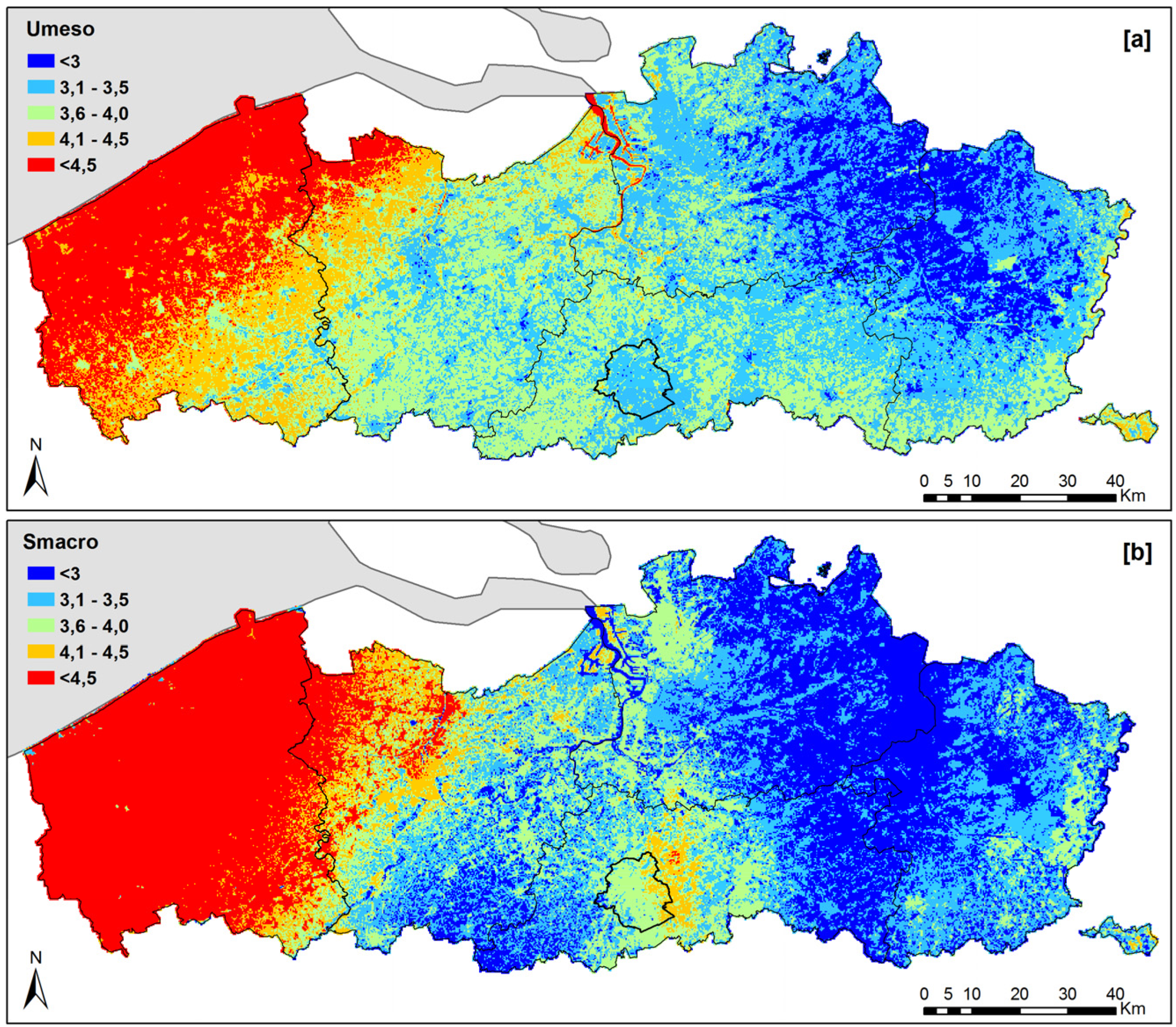
4.1. Exposure Correction

The measured surface wind speeds are used to calculate either mesowinds, U_meso, or macrowinds, S_macro, in order to correct for the influence of the terrain or local obstacles. These regional wind speeds are both interpolated by using SK before calculating the surface wind speeds at 10 m by using the roughness map. All available data summarised in Table 1 are used to create both maps. In Figure 4, the two surface wind maps resulting from the two methods are shown. Table 2 gives the statistics of the prediction errors.

From Table 2 it is clear that the methods produce very different results. The statistical values in Table 2 are all largely in favour of the U_meso method. For the S_macro method, the values indicate a larger error in the prediction map in comparison with the U_meso method. The poor results obtained here by using S_macro are in direct contrast to good results presented in [11], where the same method was applied. Two possible reasons for this difference are given. The first is that for this method the roughness has a very large influence. In this study the roughness length at the stations is obtained by using satellite images of the sites and updated pictures of the surrounding areas, identifying the relative land use. In a second step, the land uses derived were assigned their relative roughness through the use of roughness tables available in literature [25]. However, in [11] the roughness lengths at the masts are determined by analysing the wind gust ratio. This method is more accurate and less dependent on the exact mast location. Another reason is that the relationship between the mesoscale wind and the macrowind is based on the PBL similarity theory, which assumes a homogeneous PBL with neutral stability. However, in coastal areas horizontal temperature gradients are present and the method is unlikely to be applicable [12]. This may explain the failure of this method since the wind climate in Flanders is heavily determined by the presence of the sea. On the other hand, the U_meso exposure correction model gives much better results. It is expected that the results will even ameliorate when only recent observations recorded in Table 1 are used. Therefore, it was decided to use the recent data, together with the U_meso method, for the evaluation of the interpolation methods.

Figure 4. Yearly mean surface wind speed generated using the mesowind method and the macrowind method (a) Mesoscale wind interpolation. (b) Macroscale wind interpolation.

Figure 4. Yearly mean surface wind speed generated using the mesowind method and the macrowind method (a) Mesoscale wind interpolation. (b) Macroscale wind interpolation.

Table 2. Statistical details of the measurement errors for the U_meso and S_macro exposure correction methods.

Method	ME [m/s]	MAPE [%]	RMSE [m/s]	R2
Umeso	−0.069	13.82	0.596	0.68
Smacro	0.035	19.42	0.945	0.56

Table 2. Statistical details of the measurement errors for the U_meso and S_macro exposure correction methods.

Method	ME [m/s]	MAPE [%]	RMSE [m/s]	R2
Umeso	−0.069	13.82	0.596	0.68
Smacro	0.035	19.42	0.945	0.56

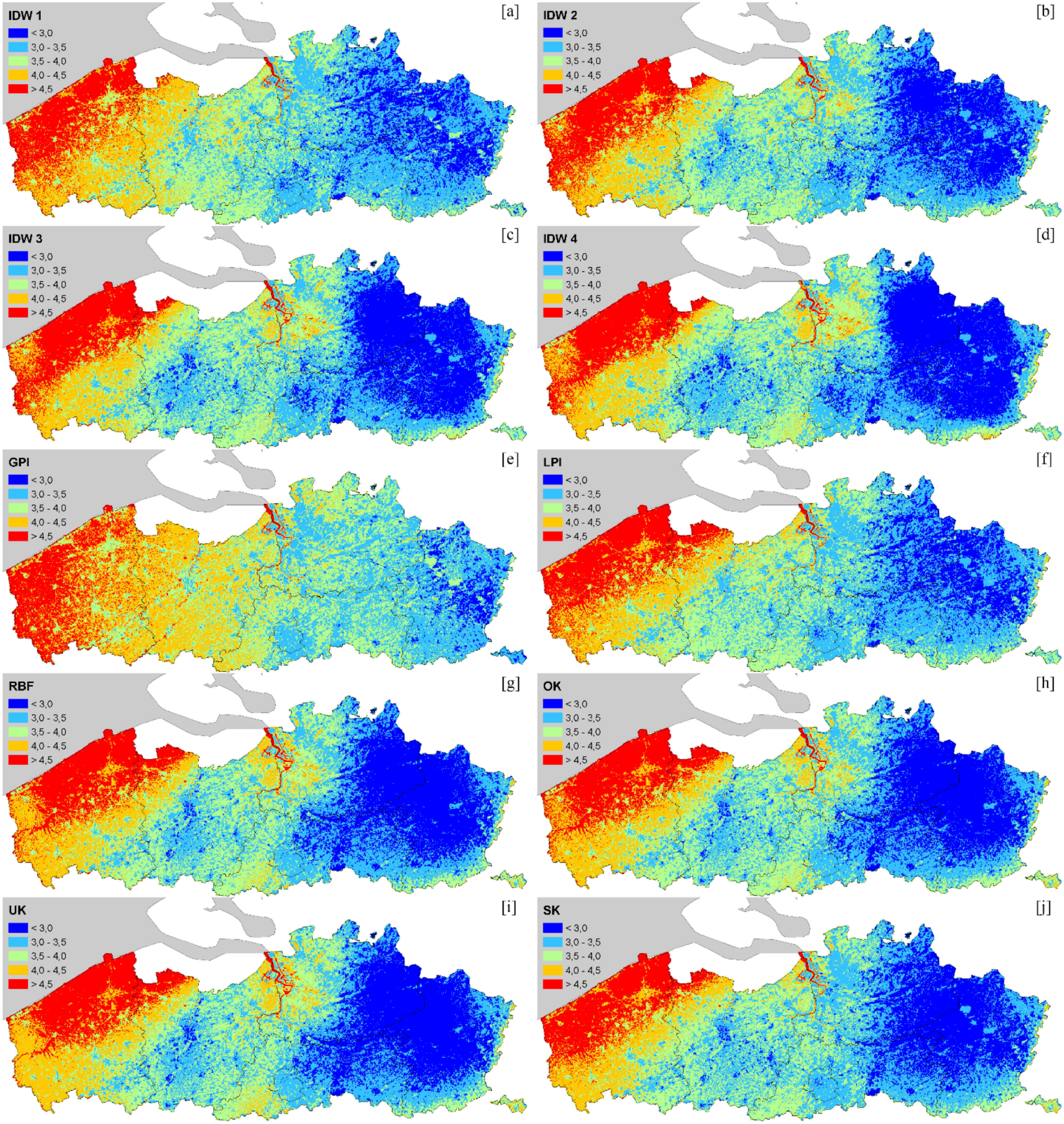
4.2. Spatial Interpolation Methods Comparison

The comparison of different interpolation methods is here presented, showing differences in the yearly mean surface wind speed, with a direct consequence on turbine sitting. The annual mean wind speed maps generated with the different interpolation methods are all shown in Figure 5. The evaluation of the results is again done by comparing the LOOCV validation statistics and is summarised in Table 3.

Figure 5. Yearly mean surface wind speed generated using different spatial interpolation methods. (a) Inverse Distance Weighted IDP = 1. (b) Inverse Distance Weighted IDP = 2. (c) Inverse Distance Weighted IDP = 3. (d) Inverse Distance Weighted IDP = 4. (e) Global Polynomial Interpolation. (f) Local Polynomial Interpolation. (g) Radial Basic Function. (h) Ordinary Kriging. (i) Universal Kriging. (j) Simple Kriging.

Figure 5. Yearly mean surface wind speed generated using different spatial interpolation methods. (a) Inverse Distance Weighted IDP = 1. (b) Inverse Distance Weighted IDP = 2. (c) Inverse Distance Weighted IDP = 3. (d) Inverse Distance Weighted IDP = 4. (e) Global Polynomial Interpolation. (f) Local Polynomial Interpolation. (g) Radial Basic Function. (h) Ordinary Kriging. (i) Universal Kriging. (j) Simple Kriging.

When comparing the statistics from SK where only recent data are used (Table 3) with the SK results where all data are used (Table 2), it is clear that the use of recent, overlapping data is most effective.

The results from IDW are largely dependent on the IDP value. The IDP = 3 is the power factor with the best overall performance. The GPI produces the most inaccurate results, with the highest RMSE and MAPE values and a large over-prediction. The LPI method also has a large negative ME value but the other statistical values are somewhat better. This is due to the fact that the mesoscale is smaller than the area of Flanders and hence GPI is not applicable here.

It can be seen that the Kriging methods and the RBF method yield very good results: they all have an RMSE value of about 0.48 m/s. OK and UK give similar results, with UK being slightly better than OK. This is caused by the fact that in Flanders a linear trend of the wind speed can be assumed, with higher values near the sea and decreasing values farther inland; this is a trend that can be incorporated in the UK method. Still, the RBF and SK methods rendered an even smaller MAPE value of 0.5%.

Table 3. LOOCV statistical values for the different spatial interpolation methods.

Method	ME [m/s]	MAPE [%]	RMSE [m/s]	R2
IDW 1	−0.143	14.58	0.577	0.56
IDW 2	−0.127	13.06	0.520	0.64
IDW 3	−0.121	12.10	0.509	0.67
IDW 4	−0.125	11.93	0.521	0.68
IDW 5	−0.132	12.29	0.540	0.68
GPI	−0.258	17.43	0.688	0.43
LPI	−0.257	13.15	0.504	0.77
RBF	−0.125	10.88	0.479	0.74
SK	−0.030	10.82	0.484	0.67
OK	−0.133	11.37	0.487	0.72
UK	−0.144	11.38	0.477	0.72

Table 3. LOOCV statistical values for the different spatial interpolation methods.

Method	ME [m/s]	MAPE [%]	RMSE [m/s]	R2
IDW 1	−0.143	14.58	0.577	0.56
IDW 2	−0.127	13.06	0.520	0.64
IDW 3	−0.121	12.10	0.509	0.67
IDW 4	−0.125	11.93	0.521	0.68
IDW 5	−0.132	12.29	0.540	0.68
GPI	−0.258	17.43	0.688	0.43
LPI	−0.257	13.15	0.504	0.77
RBF	−0.125	10.88	0.479	0.74
SK	−0.030	10.82	0.484	0.67
OK	−0.133	11.37	0.487	0.72
UK	−0.144	11.38	0.477	0.72

It is difficult to prefer one of the latter two methods over the other without additional verification measurements since the RBF method has a better R²-value but with SK, the ME value is closer to 0. Nevertheless, the under-prediction of the wind speed when using the RBF method is undesirable since it leads to an underestimation of the power production by a potential wind turbine. When comparing the maps (g) and (j) from Figure 5, the largest difference between the two interpolation methods is situated around Antwerp, where RBF predicts higher wind speeds than SK. This is due to the high wind speed recorded in Deurne (Antwerp city district) which has a higher influence on the RBF interpolation as it is an exact method. Hence, the predicted surface is forced through the measured points and thus the SK method is considered more robust and more suited to deal with wind speed measurement uncertainties.

As the station of Brasschaat (Table 1) in the Antwerp region only has recorded data up to 2006, it is not used for the construction of the wind speed maps but can be applied for evaluation of both maps. For Brasschaat, the RBF and SK methods predicted a mean wind speed of 3.40 m/s and 3.21 m/s, respectively. Knowing that the average measured wind speed from 1973 to 2006 in Brasschaat is 3.26 m/s, the prediction error equals to 4.20% for RBF and 1.36% for SK. Hence, it is demonstrated that SK has the best performance for this observation point, with RBF acting as a valuable alternative method since a small margin of error is equally observed.

The above reasoning leads to the conclusion that the SK spatial interpolation method is slightly more realistic than RBF for the interpolation of the annual mean wind speed in Flanders. With the method described above, it is possible to create wind resource maps on different heights (see Figure 6).

Figure 6. Annual mean wind speed, (a) 15 m, (b) 20 m, (c) 30 m, (d) 40 m.

Figure 6. Annual mean wind speed, (a) 15 m, (b) 20 m, (c) 30 m, (d) 40 m.

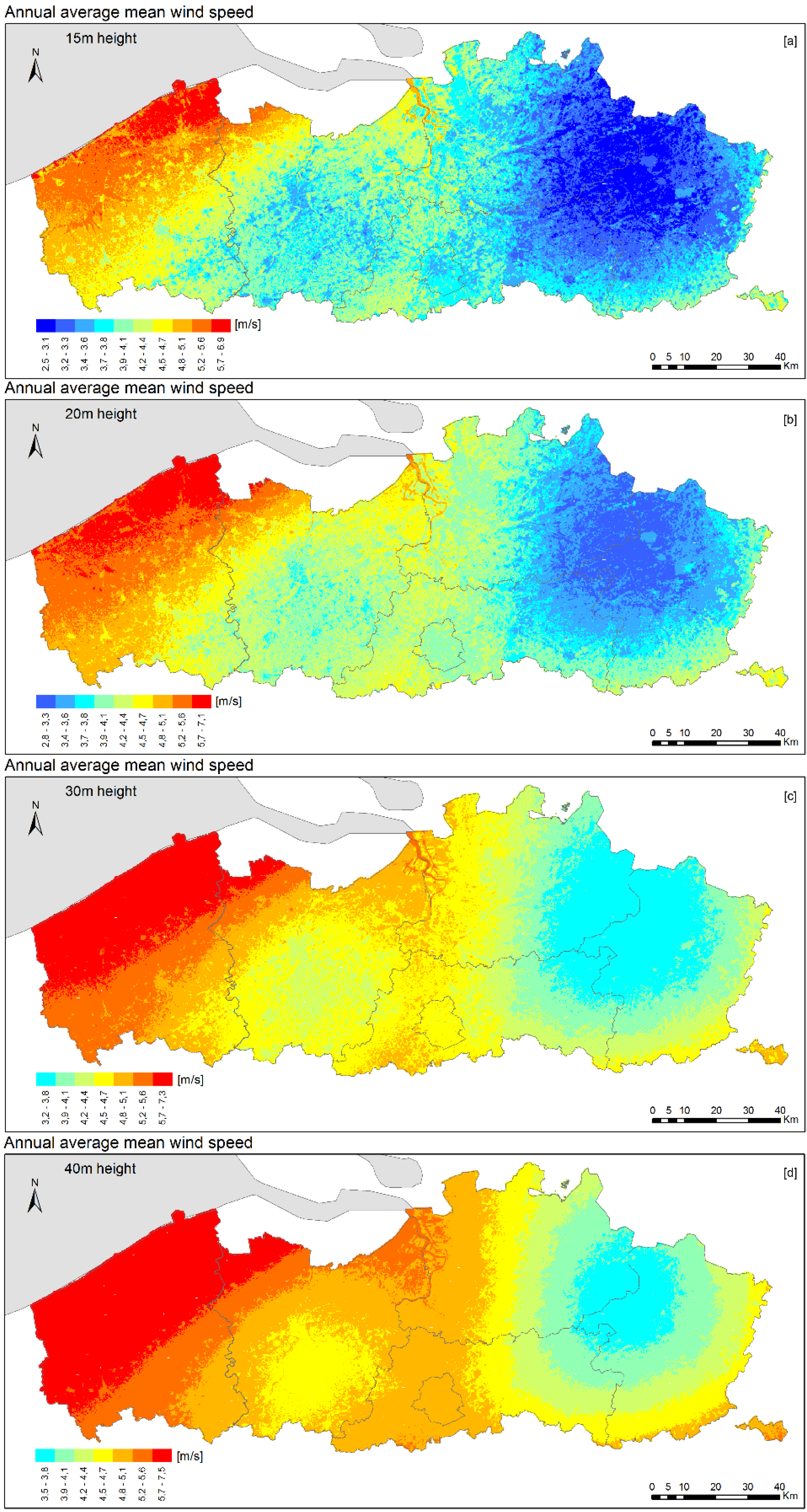
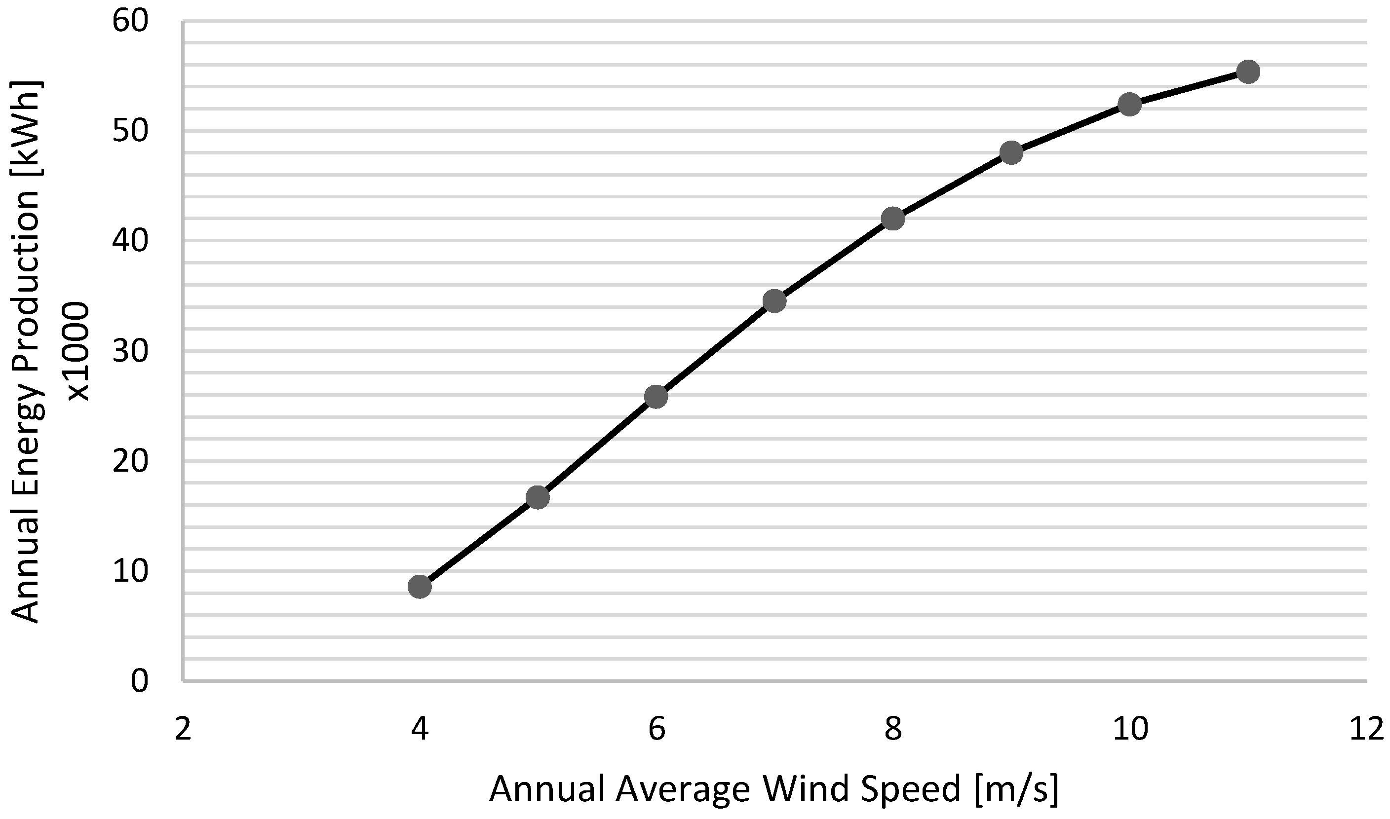
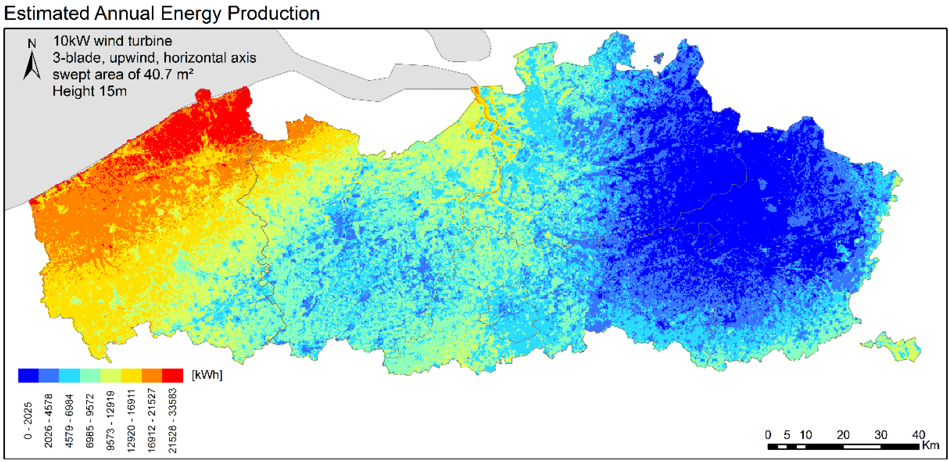
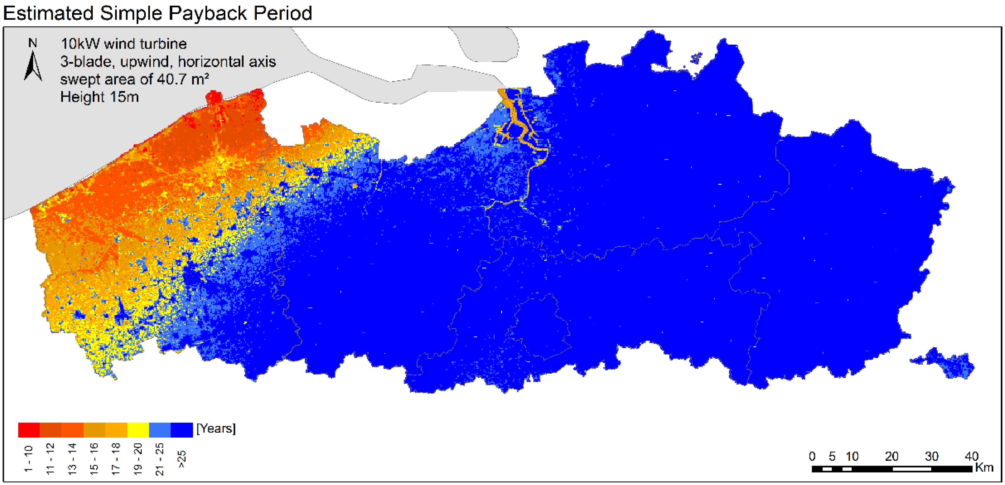
5. Energy Resource Mapping

Mean wind speed is not a representative value for energy production assessment by itself. Accordingly, in this section we use a Rayleigh distribution as an indicator to estimate energy yield, which is a Weibull distribution with a shape factor of 2 [51,52,53,54].

The International Standard IEC 61400-12-1 [55] describes methods for determining the power performance of electricity producing horizontal axis wind turbines. The annual energy production (AEP) curve, described in this standard, allows the estimation of the annual production at different reference wind speed frequency distributions, assuming 100 % availability. A Rayleigh distribution, which is identical to a Weibull distribution with a shape factor of 2, is used as the reference wind speed frequency distribution. Starting from the wind speed map of Flanders, energy resource maps could be developed for different wind turbines, based on their AEP curve (see Figure 7). In order to demonstrate how the AEP can be calculated, in this article an AEP map is created for a 10 kW 3-blade, upwind, horizontal axis wind turbine.

Figure 7. Estimated Annual Energy Production for a 10 kW 3-blade, upwind, horizontal axis wind turbine (reference air density: 1.225 kg/m³).

Figure 7. Estimated Annual Energy Production for a 10 kW 3-blade, upwind, horizontal axis wind turbine (reference air density: 1.225 kg/m³).

The horizontal axis wind turbine in this example has a swept area of 40.7 m². The above-described small wind turbine (SWT) is certified by the Small Wind Certification Council to be in conformance with the American Wind Energy Association (AWEA) Small Wind Turbine Performance and Safety Standard (AWEA Standard 9.1–2009) [56].

The equation of the best-fit curve needs to be calculated. With this, it becomes possible to calculate the estimation of the AEP in Flanders for this wind turbine (See Figure 8). This is the equation for the best fit curve:

AEP = −1 × 10⁻⁵ x⁶ – 0.0011x⁵ + 0.0696x⁴ − 1.3928x³ + 12.477x² – 42.413x + 51.124

(15)

with x representing the annual average wind speed (m/s), and taking into account the cut-in wind speed of 2.2 m/s.

In Figure 9 the estimated simple payback period is visualised for the above-described SWT. Hence it is possible to predict an area with reasonable payback times for the wind turbine. In Figure 9 only red to orange areas yield payback times that are commercially acceptable; the blue area is ruled out for the concerned SWT at a height of 15 m.

Figure 8. Estimated annual energy production (kWh) for a 10 kW 3-blade, upwind, horizontal axis wind turbine at 15 m height.

Figure 8. Estimated annual energy production (kWh) for a 10 kW 3-blade, upwind, horizontal axis wind turbine at 15 m height.

Figure 9. Estimated simple payback period (years).

Figure 9. Estimated simple payback period (years).

6. Conclusions

The present study has produced a reliable wind speed map of Flanders based on measurement data and roughness maps, and likewise has provided insight on spatial interpolation methods. The study demonstrated how local wind conditions, and thus the local wind energy generation potential, can be calculated by modelling available wind measurements.

The method used is based on a traditional wind mapping methodology but adds an integrated spatial interpolation and transformation model to create reliable location-specific wind resource maps.

By applying the model to Flanders, it was observed that transformation of the surface wind to the mesoscale level yielded better results for wind resource mapping than the macroscale level. Likewise, the comparison of seven different spatial interpolation methods led to the observation that geostatistical and RBF methods outperformed IDW and Polynomial interpolation methods.

In contrast to the findings of [11,37,38,47], the robust Simple Kriging interpolation method was found to produce the best results for developing regional wind resource maps since it has the lowest MAPE, a very low RMSE of 0.48 m/s and a negligible bias (see Table 3).

As an overall conclusion, based on statistical analysis, it was found that the transformation of surface wind measurements into mesoscale wind data in combination with Simple Kriging interpolation is the most adequate method to create reliable wind resource maps that enable the selection of optimal production sites for SMWTs in Flanders.

A limitation of the study is that an average wind speed map alone is not sufficient for wind energy applications. Accordingly, further steps for research might include additional information, such as seasonal maps and statistics on diurnal variability, to improve the energy map applications.

Another open issue is the transferability of our results, and to what extent this application for Flanders can be used as a reference for other implementations. Further steps for research should analyse whether phenomena described in the study are general characteristics under the practical applications.

References

1. Giacomarra, M.; Bono, F. European Union commitment towards RES market penetration: From the first legislative acts to the publication of the recent guidelines on State aid 2014/2020. Renew. Sustain. Energy Rev. 2015, 47, 218–232. [Google Scholar] [CrossRef] [Green Version]
2. Hanslian, D.; Hošek, J. Combining the VAS 3D interpolation method and Wind Atlas methodology to produce a high-resolution wind resource map for the Czech Republic. Renew. Energy 2015, 77, 291–299. [Google Scholar] [CrossRef]
3. Tempels, B.; Pisman, A. Open Ruimte in Verstedelijkt Vlaanderen: Een Vergelijkende Studie Naar Vier Onderschatte Ruimtegebruiken. Ruimte Maatsch. 2013, 5, 33–58. [Google Scholar]
4. VMM. Luchtkwaliteit in het Vlaamse Gewest—Jaarverslag Immissiemeetnetten; Vlaamse Milieumaatschappij: Erembodegem, Belgium, 2014. (In Dutch) [Google Scholar]
5. Ministerie van de Vlaamse Gemeenschap, afdeling Natuurlijke Rijkdommen en Energie. Windenergie Winstgevend; Ministerie van de Vlaamse Gemeenschap, afdeling Natuurlijke Rijkdommen en Energie: Brussel, Belgium, 1998; p. 16. Available online: http://stro.vub.ac.be/wind/windenergie_winstgevend.pdf (accessed on 12 August 2015). (In Dutch)
6. National Oceanic & Atmospheric Administration (NOAA). U.S. Daily Observational Data. NOAA: Washington, DC, USA. Available online: http://gis.ncdc.noaa.gov/map/viewer/#app=cdo (accessed on 12 August 2015).
7. Pryor, S.; Barthelmie, R. Climate change impacts on wind energy: A review. Renew. Sustain. Energy Rev. 2010, 14, 430–437. [Google Scholar] [CrossRef]
8. Antrop, M. Landscape change and the urbanization process in Europe. Landsc. Urban Plan. 2004, 67, 9–26. [Google Scholar] [CrossRef]
9. Silva, J.; Ribeiro, C.; Guedes, R. Roughness length classification of Corine Land Cover classes. In Proceedings of the European Wind Energy Conference, Milan, Italy, 7–10 May 2007; pp. 1–10.
10. NGI. De eenheid beeldverwerking van het NGI. Available online: http://www.ngi.be/Common/articles/CA_Td/artikel_td.htm (accessed on 12 August 2015). (In Dutch)
11. Stepek, A.; Wijnant, I.L. Interpolating Wind Speed Normals from the Sparse Dutch Network to a High Resolution Grid Using Local Roughness from Land Use Maps; Koninklijk Nederlands Meteorologisch Instituut: De Bilt, The Netherlands, 2011. [Google Scholar]
12. Wieringa, J. Roughness-dependent geographical interpolation of surface wind speed averages. Quart. J. R. Meteorol. Soc. 1986, 112, 867–889. [Google Scholar] [CrossRef]
13. Verkaik, J. Evaluation of two gustiness models for exposure correction calculations. J. Appl. Meteorol. 2000, 39, 1613–1626. [Google Scholar] [CrossRef]
14. Verkaik, J. A Method for the Geographical Interpolation of Wind Speed over Heterogeneous Terrain; Koninklijk Nederlands Meteorologisch Instituut: De Bilt, The Netherlands, 2001. [Google Scholar]
15. Verkaik, J.; Smits, A. Interpretation and estimation of the local wind climate. In Proceedings of the 3rd European & African Conference on Wind Engineering, Eindhoven, The Netherlands, 2–6 July 2001; pp. 2–6.
16. Verkaik, J.W. On Wind and Roughness over Land; Wageningen Universiteit: Wageningen, The Netherlands, 2006. [Google Scholar]
17. Verkaik, J.W. Windmodellering in het KNMI-hydra project—Opties en Knelpunten; Koninklijk Nederlands Meteorologisch Instituut: De Bilt, The Netherlands, 2000. [Google Scholar]
18. Wever, N.; Groen, G. Improving Potential Wind for Extreme Wind Statistics; Koninklijk Nederlands Meteorologisch Instituut: De Bilt, The Netherlands, 2009. [Google Scholar]
19. Lopes, A.S.; Palma, J.M.L.M.; Piomelli, U. On the Determination of Effective Aerodynamic Roughness of Surfaces with Vegetation Patches. Bound.-Layer Meteorol. 2015, 156, 113–130. [Google Scholar] [CrossRef]
20. Lorente-Plazas, R.; Montávez, J.P.; Jimenez, P.A.; Jerez, S.; Gómez-Navarro, J.J.; García-Valero, J.A.; Jimenez-Guerrero, P. Characterization of surface winds over the Iberian Peninsula. Int. J. Climatol. 2014, 35, 1007–1026. [Google Scholar] [CrossRef]
21. Baas, P.; Bosveld, F.C.; Burgers, G. The impact of atmospheric stability on the near-surface wind over sea in storm conditions. Wind Energy 2015. [Google Scholar] [CrossRef]
22. Kreibich, H.; Bubeck, P.; Kunz, M.; Mahlke, H.; Parolai, S.; Khazai, B.; Daniell, J.; Lakes, T.; Schröter, K. A review of multiple natural hazards and risks in Germany. Nat. Hazards 2014, 74, 2279–2304. [Google Scholar] [CrossRef]
23. Wieringa, J. An objective exposure correction method for average wind speeds measured at a sheltered location. Quart. J. R. Meteorol. Soc. 1976, 102, 241–253. [Google Scholar] [CrossRef]
24. Manwell, J.F.; McGowan, J.G.; Rogers, A.L. Wind Energy Explained: Theory, Design and Application; John Wiley & Sons: Hoboken, NJ, USA, 2010. [Google Scholar]
25. Wieringa, J. Representative roughness parameters for homogeneous terrain. Bound.-Layer Meteorol. 1993, 63, 323–363. [Google Scholar] [CrossRef]
26. Obukhov, A. Turbulence in an atmosphere with a non-uniform temperature. Bound.-Layer Meteorol. 1971, 2, 7–29. [Google Scholar] [CrossRef]
27. Businger, J.; Yaglom, A. Introduction to Obukhov’s paper on ‘turbulence in an atmosphere with a non-uniform temperature’. Bound.-Layer Meteorol. 1971, 2, 3–6. [Google Scholar] [CrossRef]
28. Tennekes, H. The logarithmic wind profile. J. Atmos. Sci. 1973, 30, 234–238. [Google Scholar] [CrossRef]
29. Högström, U. Von Karman’s constant in atmospheric boundary layer flow: Reevaluated. J. Atmos. Sci. 1985, 42, 263–270. [Google Scholar] [CrossRef]
30. Frenzen, P.; Vogel, C.A. A further note “on the magnitude and apparent range of variation of the von karman constant”. Bound.-Layer Meteorol. 1995, 75, 315–317. [Google Scholar] [CrossRef]
31. Garratt, J.R.; Hess, G.D.; Physick, W.L.; Bougeault, P. The atmospheric boundary layer—Advances in knowledge and application. Bound.-Layer Meteorol. 1996, 78, 9–37. [Google Scholar] [CrossRef]
32. Tieleman, H.W. Strong wind observations in the atmospheric surface layer. J. Wind Eng. Ind. Aerodyn. 2008, 96, 41–77. [Google Scholar] [CrossRef]
33. Arya, S. Suggested revisions to certain boundary layer parameterization schemes used in atmospheric circulation models. Mon. Weather Rev. 1977, 105, 215–227. [Google Scholar] [CrossRef]
34. Newman, J.F.; Klein, P.M. The impacts of atmospheric stability on the accuracy of wind speed extrapolation methods. Resources 2014, 3, 81–105. [Google Scholar] [CrossRef]
35. Duda, J.D. A Modelling Study of PBL Heights. 2010. Available online: http://www.meteor.iastate.edu/~jdduda/portfolio/605_paper.pdf (accessed on 12 August 2015).
36. Apaydin, H.; Sonmez, F.K.; Yildirim, Y.E. Spatial interpolation techniques for climate data in the GAP region in Turkey. Clim. Res. 2004, 28, 31–40. [Google Scholar] [CrossRef]
37. Cellura, M.; Cirrincione, G.; Marvuglia, A.; Miraoui, A. Wind speed spatial estimation for energy planning in Sicily: Introduction and statistical analysis. Renew. Energy 2008, 33, 1237–1250. [Google Scholar] [CrossRef]
38. Chinta, S. A Comparison of Spatial Interpolation Methods in Wind Speed Estimation across Anantapur District, Andhra Pradesh. J. Earth Sci. Res. 2014, 2, 48–54. [Google Scholar] [CrossRef]
39. Luo, W.; Taylor, M.; Parker, S. A comparison of spatial interpolation methods to estimate continuous wind speed surfaces using irregularly distributed data from England and Wales. Int. J. Climatol. 2008, 28, 947–959. [Google Scholar] [CrossRef]
40. Rehman, S.U.; Uddin Qazi, M.; Siddiqui, I.; Shah, N.H.S. Comparing Geostatistical and Non-geostatistical Techniques for the Estimation of Wind Potential in Un-sampled Area of Sindh, Pakistan. Eur. Acad. Res. 2013, I, 1770–1792. [Google Scholar]
41. Wei, Y. Spatial Variation and Interpolation of Wind Speed Statistics and Its Implication in Design Wind Load. Postdoctoral Thesis, The University of Western Ontario, London, ON, Canada, 2013. [Google Scholar]
42. Dobesch, H.; Dumolard, P.; Dyras, I. Spatial Interpolation for Climate Data: The Use of GIS in Climatology and Meteorology; John Wiley & Sons: Hoboken, NJ, USA, 2013. [Google Scholar]
43. Michaelsen, J. Cross-validation in statistical climate forecast models. J. Clim. Appl. Meteorol. 1987, 26, 1589–1600. [Google Scholar] [CrossRef]
44. Keckler, D. The Surfer Manual; Golden Software, Inc.: Golden, CO, USA, 1995. [Google Scholar]
45. Song, J.; DePinto, J.V. A GIS-based Data Quer y System. In Proceedings of the International Association for Great Lakes Research (IAGLR) Conference, Windsor, ON, Canada, 10–14 January 1995.
46. Johnston, K.; ver Hoef, J.M.; Krivoruchko, K.; Lucas, N. Using ArcGIS Geostatistical Analyst; ESRI: Redlands, CA, USA, 2001; p. 300. [Google Scholar]
47. Ali, S.M.; Mahdi, A.S.; Shaban, A.H. Wind Speed Estimation for Iraq using several Spatial Interpolation Methods. Br. J. Sci. 2012, 7, 48–55. [Google Scholar]
48. Lang, C.-Y.; de Mesnard, L. Types of Interpolation Methods. Available online: http://www.gisresources.com/types-interpolation-methods_3/ (accessed on 3 July 2015).
49. Shi, G. Chapter 8—Kriging Data Mining and Knowledge Discovery for Geoscientists; Elsevier: Amsterdam, The Netherlands, 2014; pp. 238–274. [Google Scholar]
50. Eberly, S.; Swall, J.; Holland, D.; Cox, B.; Baldridge, E. Developing Spatially Interpolated Surfaces and Estimating Uncertainty; United States Environmental Protection Agency: Washington, DC, USA, 2004.
51. Alodat, M.T.; Anagreh, Y.N. Durations distribution of Rayleigh process with application to wind turbines. J. Wind Eng. Ind. Aerodyn. 2011, 99, 651–657. [Google Scholar] [CrossRef]
52. Olaofe, Z.O.; Folly, K.A. Statistical Analysis of Wind Resources at Darling for Energy Production. Int. J. Renew. Energy Res. 2012, 2, 250–261. [Google Scholar]
53. Olaofe, Z.O.; Folly, K.A. Wind energy analysis based on turbine and developed site power curves: A case-study of Darling city. Renew. Energy 2013, 53, 306–318. [Google Scholar] [CrossRef]
54. Ahmmad, M.R. Statistical Analysis of the Wind Resources at the Importance for Energy Production in Bangladesh. Int. J. U- & E-Service Sci. Technol. 2014, 7, 127–136. [Google Scholar]
55. IEC. International Standard IEC 61400-12-1. Available online: ftp://ftp.ee.polyu.edu.hk/wclo/Ext/OAP/IEC61400part12_1_WindMeasurement.pdf (accessed on 12 August 2015).
56. AWEA Small Wind Turbine Performance and Safety Standard; American Wind Energy Association: Washington, DC, USA, 2009.
57. Van Ackere, S.; van Wyngene, K. Windkracht 13. Available online: http://www.windkracht13.be/ (accessed on 3 July 2015).
58. Van Eetvelde, G.; van Zwam, B.; Maes, T.; Vollaard, P.; De Vries, I.; Tavernier, P.; D’Hooge, E.; Geenens, D.; Verdonck, L.; Leynse, L. Praktijkboek duurzaam bedrijventerreinmanagement; POM West-Vlaanderen: Sint-Andries, Belgium, 2008; p. 117. (In Dutch) [Google Scholar]