Article

Enhanced Predictive Current Control of Three-Phase Grid-Tied Reversible Converters with Improved Switching Patterns

1
Department of Electrical Engineering and Automation, Tianjin University, Tianjin 30072, China
2
Department of Energy Technology, Aalborg University, Aalborg 9220, Denmark
3
Faculty of Science and Engineering, University of Chester, Chester CH1 4BJ, UK
*
Author to whom correspondence should be addressed.
These authors contributed equally to this work.
Energies 2016, 9(1), 41; https://doi.org/10.3390/en9010041
Submission received: 2 November 2015 / Revised: 1 December 2015 / Accepted: 30 December 2015 / Published: 13 January 2016

Abstract

:
A predictive current control strategy can realize flexible regulation of three-phase grid-tied converters based on system behaviour prediction and cost function minimization. However, when the predictive current control strategy with conventional switching patterns is adopted, the predicted duration time for voltage vectors turns out to be negative in some cases, especially under the conditions of bidirectional power flows and transient situations, leading to system performance deteriorations. This paper aims to clarify the real reason for this phenomenon under bidirectional power flows, i.e., rectifier mode and inverter mode, and, furthermore, seeks to propose effective solutions. A detailed analysis of instantaneous current variations under different conditions was conducted. An enhanced predictive current control strategy with improved switching patterns was then proposed. An experimental platform was built based on a commercial converter produced by Danfoss, and moreover, relative experiments were carried out, confirming the superiority of the proposed scheme.

1. Introduction

During the past few decades, a large variety of active systems have been connected to the electric power system, including geothermal generators, photovoltaic systems, wind turbines, and so on. Most of these installations are connected to the grid with the assistance of grid-tied converters. Consequently, flexible interconnections of different installations depend largely on the design and control of grid-tied converters. In the past few years, model predictive control (MPC) of converters has received significant attention and experienced sustained development [1]. Various types of model predictive controllers have emerged as effective strategies and promising alternatives for the control of power converters and electrical machines [2,3,4,5,6,7,8,9,10,11,12]. One feasible solution for the application of MPC is known as continuous set model predictive control [13,14]. Continuous voltage reference signals are obtained by means of online optimization and cost function minimization. A modulator is normally required to generate the switching signals. With continuous set model predictive strategies adopted, control actions are considered to be continuous. By contrast, another approach called finite set model predictive control regards these discrete switching actions as the constraints of the system inputs [15,16]. During the optimizing process, the control actions are constrained to the limited available switching states, instead of continuous sets [17,18,19]. Until recently, finite set model predictive control with one-step prediction horizons has been applied to various converter topologies and also with a wide range of control objectives, including speed control, current control, power control, torque and flux control [20,21,22,23,24].
As demonstrated by recent research, finite set model predictive control outperforms classical linear solutions with regard to transient behaviours and control flexibility [25,26]. Meanwhile, a relative amount of research has been conducted in order to overcome some of the shortcomings possessed by the finite set model predictive control technique, including unsatisfactory steady-state performances, variable switching frequency and the wide distributed spectra of output waveforms. A large number of novel solutions to these practical problems have been reported. Several constant-switching frequency MPC strategies were developed, by means of introducing frequency information to the cost function or the adoption of a modulation stage. However, even though the desired switching patterns and spectrum distribution can both be achieved, transient performances were deteriorated due to the low-pass filter characteristics possessed by these methods. In [27,28], two active vectors were firstly selected during each sampling interval. An optimal vector sequence was then symmetrically built up on the basis of one zero vector and two selected vectors. With the assistance of cost function minimization, the application times of each vector element in the optimal sequence were finally determined. This is quite different from the working principle of finite set model predictive control techniques, in which the optimal switching action is selected and, in particular, remains fixed within each sampling interval once it is determined. Note that when the method proposed in [27,28] is adopted, the predicted application times of each vector element in the optimal sequence might be smaller than zero. In reality, the application times of voltage vectors or switching states should never be negative. This item should be taken into consideration when the algorithm is implemented. Recently, this has been paid special attention to, and several improved versions of this control methodology have been proposed [4,28,29,30,31,32]. In [4], a generalized predictive direct power control strategy was proposed. The cost function was calculated for each sector. Based on cost function comparisons, the optimal voltage vectors and their time sequences are finally determined. Even though a corresponding simplified scheme was further proposed, the cost function still needs to be calculated six times within each sampling period [19]. In [30], the calculated values of the predicted application time are firstly examined. Whenever the application time is less than zero, the optimal voltage vector sequences were to be modified according to a pre-defined switching table. Nevertheless, even though steady-state performance deteriorations can be successfully suppressed, those transient performance deteriorations caused by the incorrect selection of voltage vectors were not paid attention to. Besides, transient performance deterioration caused by the negative duration times also was not mentioned or analysed in previous studies [30,31,32]. Besides, the research conducted in [31,32] only refers to the control actions when the converter is operating in the rectifier mode. The corresponding control problem under the situation of reversible power flows was not properly solved.
This paper aims to reveal the reason for the operating characteristics under bidirectional power flows, i.e., rectifiers and inverters, and, furthermore, seeks to propose effective solutions. The following sections are organized as follows. In Section 2, the operating principle of conventional predictive current control for three-phase grid-tied reversible converters is briefly depicted. A detailed analysis is then conducted in Section 3 with its shortcomings emphasized, and an enhanced strategy with improved switching patterns is developed. In order to demonstrate the main advantage of the proposed enhanced predictive current control strategy, Section 4 presents comparative experimental results based on a commercial grid-tied converter produced by Danfoss Company. Conclusions are finally presented in Section 5.

2. Operating Principle of Predictive Current Control for Three-Phase Grid-Tied Reversible Converters

In this section, it is assumed that the three-phase grid-tied reversible converter operates in the rectifier mode. In the synchronous reference frame, the instantaneous variations of the converter current within each sampling period can be written as:
Δ I g = d I g d t = 1 L g ( U g R g I g j ω L g I g U c )
where Ug represents the grid voltage vector and Uc is the converter output voltage vector; Ig is the converter current vector; ω, Lg and Rg denote the angular frequency of grid voltage, the line inductance and its equivalent resistance, respectively.
Normally, two adjacent voltage vectors should be firstly selected as active vectors according to the angular location of Ug [33]. These two selected active vectors will be applied together with the zero vector V0,7. For the purposes of convenience, Vm and Vn are adopted to denote the first and second vectors, respectively. Their application times tm and tn will be further determined by minimizing a pre-defined cost function.
Taking Sector 6, for example, V6 and V1 should be selected when Ug is located in this sector. These two vectors will then be applied along with the zero vector V0,7. When different voltage vectors are applied, the instantaneous current variation differs accordingly. The instantaneous current variations resulting from the application of V1, V6 and V0,7 can be predicted as:
Δ I g - V 1 = 1 L g ( U g R g I g j ω L g I g V 1 )
Δ I g - V 6 = 1 L g ( U g R g I g j ω L g I g V 6 )
Δ I g - V 0 , 7 = 1 L g ( U g R g I g j ω L g I g V 0 , 7 )
Within each sampling period Ts, the current variation ΔIg-Ts produced by the joint actions of two active vectors and the zero vector V0,7 can be predicted as:
Δ I g - T s = Δ I g - V 1 t 1 + Δ I g - V 6 t 6 + Δ I g - V 0 , 7 t 0
where t1, t6 and t0 denote the duration times of different vectors within each sampling interval Ts.
Under the joint actions of V1, V6 and V0,7, the current tracking error vector Eg at the end of the k-th sampling period can thus be computed as follows:
E g = I g I g Δ I g - T s
where Ig* is the current reference vector and Ig represents the current vector at the initial instant of the k-th sampling period.
It is hoped that the converter current evolves from the initial vector Ig toward the reference vector Ig* within one sampling period. In other words, the duration times of two active voltage vectors should be determined with the aim of eliminating the current tracking error vector Eg at the end of each sampling period [34]. Conventionally, the optimal duration values of t1 and t6 satisfy the following minimum value condition:
W t 1 = W t 6 = 0
where W denotes the cost function given by:
W = | E g | 2
Based on Equation (7), the optimal duration times for two active vectors can be calculated and applied accordingly. It should be noted that Sector 6 is taken as an example here. When Ug is located in other sectors, the selected active voltage vectors will change accordingly.

3. Performance Analysis of the Predictive Current Control Strategy

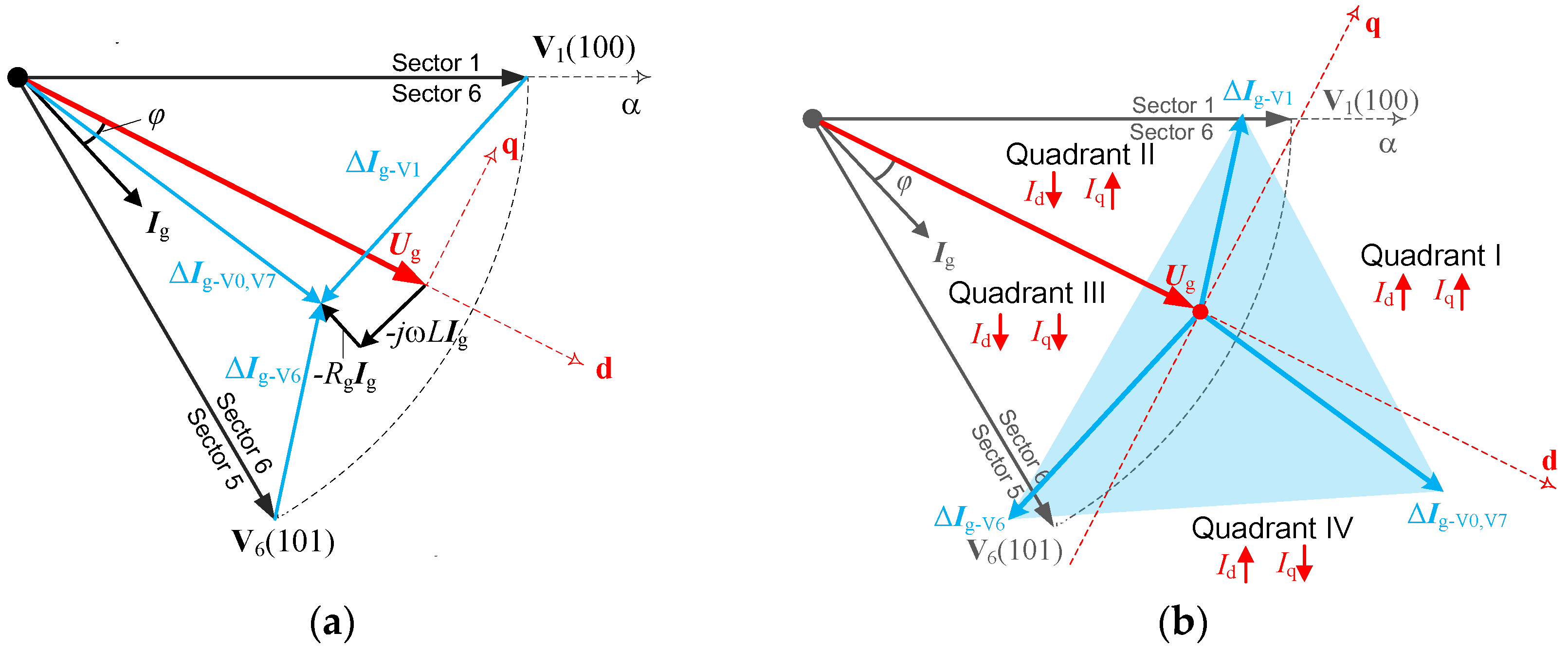
3.1. Rectifier Mode Analysis

Assuming that the three-phase grid-tied reversible converter is operating in rectifier mode, the instantaneous current variations caused by the application of V6, V1 and V0,7 when Ug lies in Sector 6 is depicted in Figure 1a. After vector movement and rearrangement, instantaneous current variations in the dq-reference frame can be depicted as in Figure 1b.
Figure 1. Instantaneous current variations caused by the application of V6, V1 and V0,7 when Ug is located in the middle part of Sector 6 (Rectifier mode). (a) Original diagram; (b) Diagram after vector movement and rearrangement.
Energies 09 00041 g001
As depicted in Figure 1b, the instantaneous current variation vector ΔIg-V0,V7 resulting from the application of zero vector V0,7 lies in Quadrant IV of the dq-reference frame. This indicates that the actions of V0,7 will surely result in the increase of id, as well as the decrease of iq. Besides, as ΔIg-V1 is located in Quadrant II, the application of V1 will lead to the decrease of id and the increase of iq. Similarly, id and iq will both be decreased under the action of V6, due to the location of ΔIg-V6 in Quadrant III. Generally speaking, joint actions of V6, V1 and V0,7 can result in both an increase and a decrease of the d- and q-axes currents. In other words, the d- and q-axes currents can be properly regulated by combining the actions of V6, V1 and V0,7. Actually, this is due to the fact that the light blue area composed of three vectors ΔIg-V6, ΔIg-V1, ΔIg-V0,V7 covers four quadrants in the dq-reference frame, as can be clearly seen in Figure 1b. However, this is not the case when Ug is located in the initial part of Sector 6, as shown in Figure 2.
Figure 2. Instantaneous current variations caused by the application of V6, V1 and V0,7 when Ug is located in the initial part of Sector 6 (rectifier mode). (a) Original diagram; (b) Diagram after vector movement and rearrangement.
Energies 09 00041 g002
As shown in Figure 2, the light blue area composed of three vectors ΔIg-V6, ΔIg-V1, ΔIg-V0,V7 only covers Quadrants III and IV in the dq-reference frame. The actions of V0,7 and V1 both result in the increase of id and the decrease of iq. The application of V6 will lead to the decrease of the d- and q-axes currents. Obviously, iq can only be decreased by the joint actions of V6, V1 and V0,7. It is found that, under this situation, the duration time t1 of the selected voltage vector V1, which is calculated based on cost function minimization, will turn out to be negative. With common sense, the duration time of voltage vectors should not be a negative value and will be forced to zero. Under this situation, the flexible regulation of currents cannot be successfully achieved. Actually, V1 and V5 should be chosen and applied under this situation, instead of V1 and V6. In order to clarify this remarkable conclusion, Figure 3 demonstrates the instantaneous current variations caused by the application of V5, V6 and V0,7 when Ug is located in the initial part of Sector 6.
Figure 3. Instantaneous current variations caused by the application of V5, V6 and V0,7 when Ug is located in the initial part of Sector 6 (rectifier mode).
Energies 09 00041 g003
As shown in Figure 3, the light blue area composed of ΔIg-V5, ΔIg-V6, ΔIg-V0,V7 covers four quadrants in the dq-reference frame. Consequently, both an increase and a decrease of the dq-axes currents can be expected under the joint actions of V5, V6 and V0,7. Flexible regulation of currents can thus be achieved. Therefore, when Ug is located in the position as shown in Figure 3, V5 and V6 should be selected as active vectors, instead of V1 and V6. A similar conclusion can be easily obtained when Ug lies in other sectors.
Furthermore, incorrect selection of voltage vectors and negative duration time also come out when there is a step change in the reference current. Taking Sector 6 for example, the duration time t1 is negative, while t6 remains positive when the q-axis reference current is step-up changed. The reason for this phenomenon is that the selected voltage vectors V6 and V1 could not produce large current variations as desired. Under this situation, V5 and V6 should be selected and applied, instead of V6 and V1. Figure 4 depicts the instantaneous current variations caused by the application of V5 and V6 when Ug lies in Sector 6. By comparing Figure 4 with Figure 1a, it is clearly visible that the joint actions of V5 and V6 can produce much larger current variations than those of V6 and V1.
It should be noted that, as pointed out previously, even though the analysis in this section is carried out based on the example of Sector 6, the obtained conclusion can be also extended to other sectors. Besides, the calculated duration times for selected voltage vectors turn out to be negative under the situation of step change in d-axis currents. Similar analysis and the corresponding modifications of vector selection rules can be easily obtained based on previous contents.
Figure 4. Instantaneous current variations caused by the application of V5, V6 and V0,7 when Ug lies in the middle part of Sector 6 (rectifier mode).
Energies 09 00041 g004

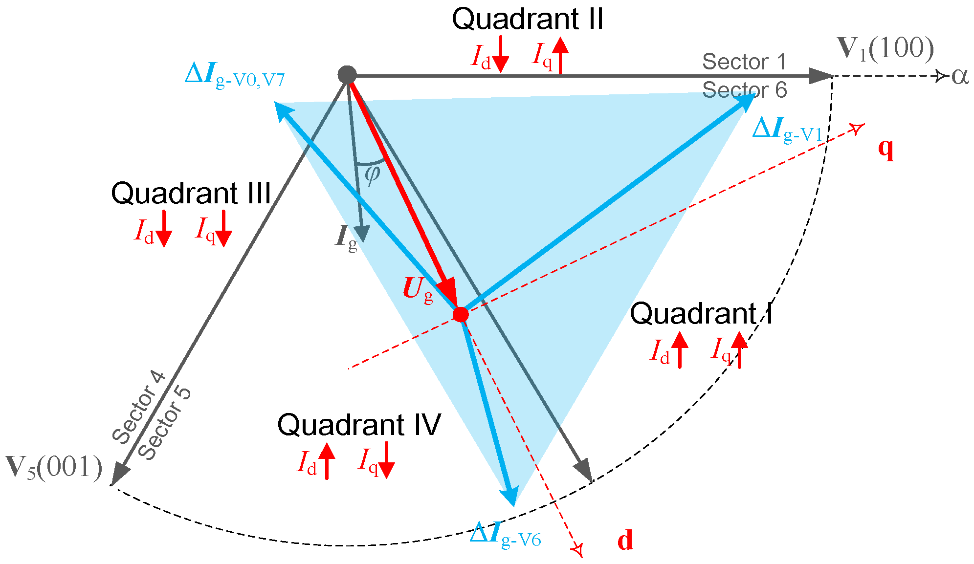
3.2. Inverter Mode Analysis

In some applications, the three-phase grid-tied converter may operate in the inverter mode. In this case, the instantaneous current variation resulting from the application of voltage vector Vi (i = 0,…,7) should be rewritten as:
Δ I g - V i = 1 L g ( V i R g I g j ω L g I g U g )
As argued previously, when the converter is operating in rectifier mode and Ug is located in the initial part of Sector 6, the predictive controller will lose its effectiveness if V1 and V6 are selected as active voltage vectors. However, this is not the case when the converter operates in the inverter mode. Figure 5 depicts instantaneous current variations when Ug lies in the initial part of Sector 6.
It can be clearly observed in Figure 5 that, when the converter is operating in the inverter mode, the highlighted blue area composed of three vectors ΔIg-V1, ΔIg-V6, ΔIg-V0,V7 covers four quadrants in the dq-reference frame. The increase and decrease of the dq-axes currents can both be achieved. Therefore, when the converter is operating in the inverter mode and Ug is located in the initial part of Sector 6, selection of V6 and V1 as active vectors can realize flexible regulation of both d- and q-axis currents. This phenomenon is quite different from that when the converter is operating in the rectifier mode, as mentioned previously.
Figure 5. Instantaneous current variations ΔIg-V6, ΔIg-V1, ΔIg-V0,V7 in the dq-reference frame when Ug is located in the initial part of Sector 6 (inverter mode). (a) Original diagram; (b) Diagram after vector movement and rearrangement.
Energies 09 00041 g005
However, when Ug is located in the latter part of each sector, incorrect selection of active vectors will come out. Taking Sector 5 for example, when Ug is located in the latter part of this sector, V5 and V6 should normally be selected and applied. Figure 6 shows the instantaneous current variations by the application of V5, V6 and V0,7.
Figure 6. Instantaneous current variations caused by the application of V5, V6 and V0,7 when Ug is located in the latter part of Sector 5 (inverter mode). (a) Original diagram; (b) diagram after vector movement and rearrangement.
Energies 09 00041 g006
It is clearly visible in Figure 6 that the light blue area composed of three vectors ΔIg-V5, ΔIg-V6, ΔIg-V0,V7 only covers Quadrants III and IV in the dq-reference frame. Even though the increase and decrease of the d-axis current can both be achieved, the q-axis current will only be decreased under the joint actions of these voltage vectors. When V5 and V6 are still selected and applied in this case, the minimization of the cost function will lead to negative duration time t5. A similar phenomenon can also be observed when Ug is located in other sectors. In general, under inverter mode, the duration time tm of the voltage vector Vm will become negative when the grid voltage vector is located in the latter part of each sector. The negative duration time will be forced to zero during the application process, resulting in performance deterioration. This will be further validated by the experimental waveforms to be presented in the following sections. It should be noted that, different from the situation of rectifier mode, as shown in Figure 2, incorrect selections of active vectors come out when Ug lies in the latter part of different sectors, instead of their initial part.
Actually, V5 should be replaced by V1 when Ug is located in the latter part of Sector 5. Subsequently, V1 is applied together with V6. In order to clarify this conclusion, Figure 7 depicts instantaneous current variations under the joint actions of V1, V6 and V0,7 when Ug is located in the latter part of Sector 5.
Figure 7. Instantaneous current variations caused by the application of V1, V6 and V0,7 when Ug is located in the latter part of Sector 5 (inverter mode).
Energies 09 00041 g007
Obviously, when V1 and V6 are selected as active vectors in this case, instantaneous current variation vectors can reach all four quadrants in the dq-reference frame. It can be inferred that the dq-axes currents can both be increased and decreased with the joint actions of V1, V6 and V0,7. Flexible regulation of converter currents can thus be achieved under this situation.
Moreover, with a step change in the reference value of currents, the selection of two adjacent vectors according to the angular location of Ug will also result in negative duration time. Again, Sector 6 is taken as an example here. When the q-axis reference current is step-up changed, the duration time t6 for voltage vector V6 is negative, while t1 for voltage vector V1 remains positive. This is because large current variations are normally desired when the reference signals are step changed. However, the joint actions of V6 and V1 could not produce such large current variations as desired. Under this situation, other combinations of voltage vectors that can generate larger current variations should be chosen and applied, instead of V6 and V1. For the purpose of illustration, Figure 8 shows instantaneous current variations caused by the joint actions of V1, V2 and V0,7 when Ug is located in Sector 6.
Figure 8. Instantaneous current variations caused by the application of V1, V2 and V0,7 when Ug is located in Sector 6 (inverter mode).
Energies 09 00041 g008
In fact, V1 and V2 should be selected when the q-axis reference current is step-up changed. This is due to fact that the combination of V1 and V2 can generate much larger positive variations of q-axis currents than the joint actions of V6 and V1. This conclusion can be easily drawn by comparing Figure 8 to Figure 5. As argued previously, the analysis in this section is based on the example of Sector 6. Similar conclusions can be easily obtained when the grid voltage vector is located in other sectors. The corresponding modifications of vector selection rules can be easily obtained based on previous contents.

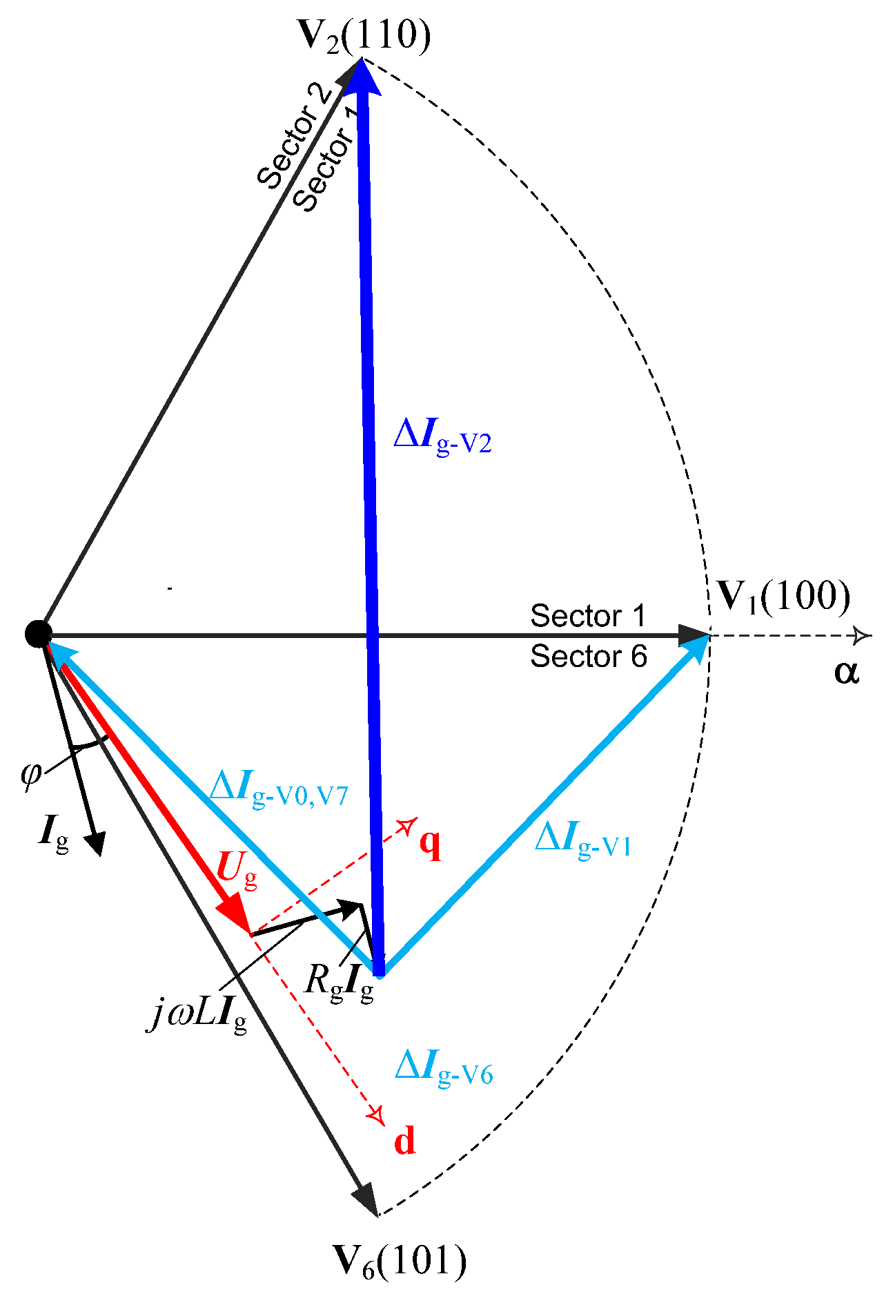
3.3. Modified Switching Patterns for Reversible Converters

Based on the analysis mentioned above, modified switching patterns for reversible converters can be summarized as Table 1. For clarity and better understanding, the improved switching patterns mentioned above can be explained as follows. Taking Sector I for example, when the grid voltage Ug is located in Sector I, two adjacent voltage vectors V1 and V2 are firstly selected. Their duration times tm (t1) and tn (t2) are then determined by minimizing the cost function. If t1 and t2 are both positive (tm > 0 and tn > 0), V1 and V2 are directly applied, as well as the zero vector V0,7. If t1 is negative while t2 keeps positive (tm < 0 and tn > 0), V2 and V3 should be chosen to replace the combination of V1 and V2. If t2 is negative while t1 remains positive (tm > 0 and tn < 0), V6 and V1 are to be applied. When t1 and t2 are both negative (tm < 0 and tn < 0), the corresponding opposite vectors to V4 and V5 should be selected in this case. Finally, the application times of re-selected vectors are then calculated based on cost function minimization.
The illustrative block diagram of the proposed control strategy is depicted in Figure 9, where the current references are obtained based on the outer voltage control loop. The pulse width modulation (PWM) block is used to generate switching signals for the converter.
Figure 9. Block diagram of the proposed control strategy.
Energies 09 00041 g009
Table 1. Improved switching patterns for the proposed strategy.
Sectortm > 0 and tn > 0tm > 0 and tn < 0tm < 0 and tn > 0tm < 0 and tn < 0
1V1, V2V6, V1V2, V3V4, V5
2V2, V3V1, V2V3, V4V5, V6
3V3, V4V2, V3V4, V5V6, V1
4V4, V5V3, V4V5, V6V1, V2
5V5, V6V4, V5V6, V1V2, V3
6V6, V1V5, V6V1, V2V3, V4

4. Experimental Validations

With the aim of comparing the performances of the proposed improved predictive control strategy with those of the conventional controller, extensive experimental research on steady-state behaviours and transient responses was carried out on a three-phase grid-tied reversible converter prototype. The parameters are listed in Table 2. Throughout the experiments, a Danfoss FC302 converter for industrial applications was used to realize reversible power conversion. Besides, a variac was adopted to connect the AC supply and the experimental prototype. The algorithm processing, AD input, DA output and pulse width modulation (PWM) generation are realized by a dSPACE DS1006 board, a DS 2004 ADC board, a DS2102 DAC board and a DS5101 PWM board, respectively. During the tests, the sampling period is chosen as 100 μs. It should be noted that, for the purposes of convenience, the conventional predictive current controller is referred to as Method I, while the proposed strategy is referred to as Method II.
Table 2. Parameters of the experimental platform.
ParameterValue
Rated power11 kW
Line-to-line voltage (Root mean squar value)245 V
Grid frequency50 Hz
Filter inductance7.8 mH
Filter resistance0.1 Ω
DC-link capacitor950 μF
Sampling period100 μs

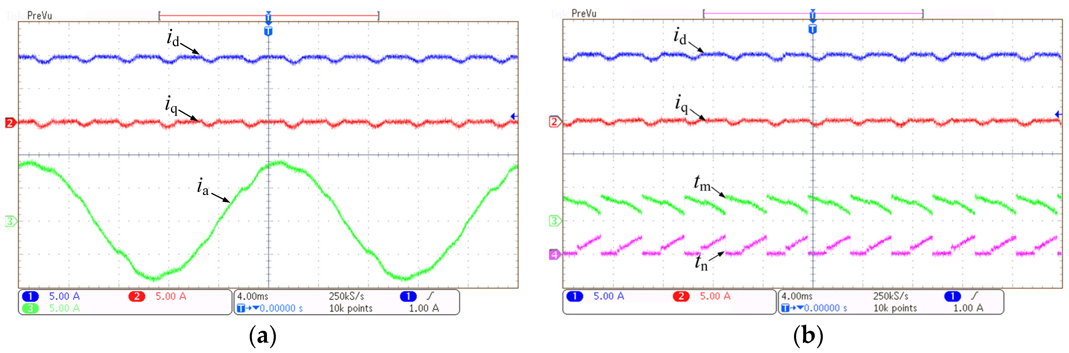
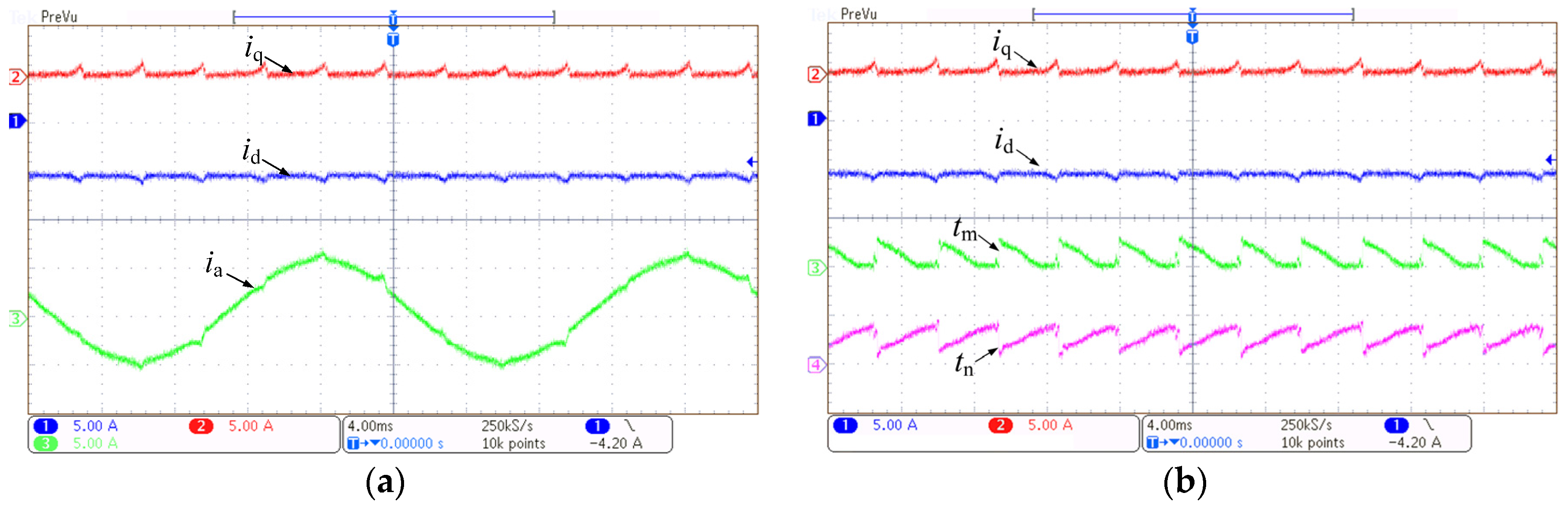
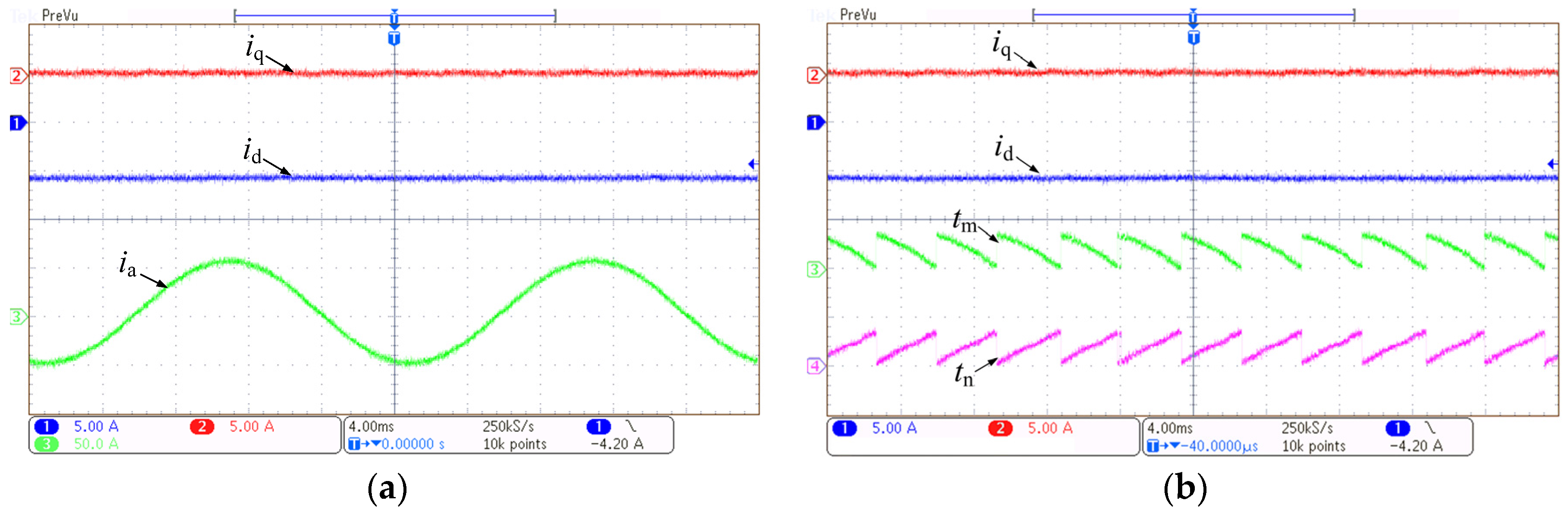
4.1. Steady-State Behaviours

When Method I is adopted, two adjacent voltage vectors are normally selected as active vectors according to the angular position of the grid voltage vector. However, this might lead to negative duration time when the cost function is minimized. Conventionally, the duration time of voltage vectors should be larger than zero. The negative duration time will thus be forced to zero. In order to evaluate its influence on system steady-state behaviours when the converter is operating in rectifier and inverter modes, relative experiments were conducted. Here, id* and iq* are used to denote the reference signals for d- and q-axis currents, respectively. As is clearly visible in Figure 10 and Figure 11, severe periodic fluctuations can be observed in both d- and q-axes currents. In other words, when the negative duration time comes out and is forced to zero, the phenomenon of control failure comes out, as shown in Figure 10b and Figure 11b. Under this situation, the dq-axis currents could not be regulated in a smooth way, therefore generating significant harmonic distortions in thephase current.
Figure 10. Experimental results: dq-axis currents, Phase A current, tm and tn (rectifier mode, Method I, id* = 10 A, iq* = 0 A). (a) dq-axis and Phase A currents; (b) tm and tn (50 μs/division).
Energies 09 00041 g010
Figure 11. Experimental results: dq-axis currents, Phase A current, tm and tn (inverter mode, Method I, id* = 6 A, iq* = 0 A). (a) dq-axis and Phase A currents; (b) tm and tn (50 μs/division).
Energies 09 00041 g011
As argued in previous sections, the control failure and performance deterioration demonstrated in Figure 10 and Figure 11 result from the incorrect selection of voltage vectors. Those two voltage vectors, which are adjacent to the grid voltage vectors, are not always the optimum vectors. Figure 12 presents experimental waveforms when the proposed Method II is adopted and the converter is operating in rectifier mode. These experimental results were obtained under the same conditions as those of Figure 10. It can be seen that the proposed Method II presents superior performances to the conventional predictive control strategy. Due to the modified switching pattern shown in Figure 12c, both tm and tn stay positive at all times when the proposed strategy is used, as shown in Figure 12b. Periodic fluctuations in the dq-axes currents are successfully eliminated as expected, and as a result, dq-axes currents can both be regulated to be smooth and constant. The sinusoidal AC current is further obtained. Similar results can be obtained when the converter is operating in inverter mode, as shown in Figure 13.
Figure 12. Experimental results: dq-axis currents, Phase A current, tm and tn (rectifier mode, Method II, id* = 10 A, iq* = 0 A). (a) dq-axis and Phase A currents; (b) tm and tn (50 μs/division); (c) selected voltage vectors.
Energies 09 00041 g012
Figure 13. Experimental results: dq-axis currents and Phase A current (inverter mode, Method II, id* = 6 A, iq* = 0 A). (a) dq-axis and Phase A currents; (b) tm and tn (50 μs/division).
Energies 09 00041 g013

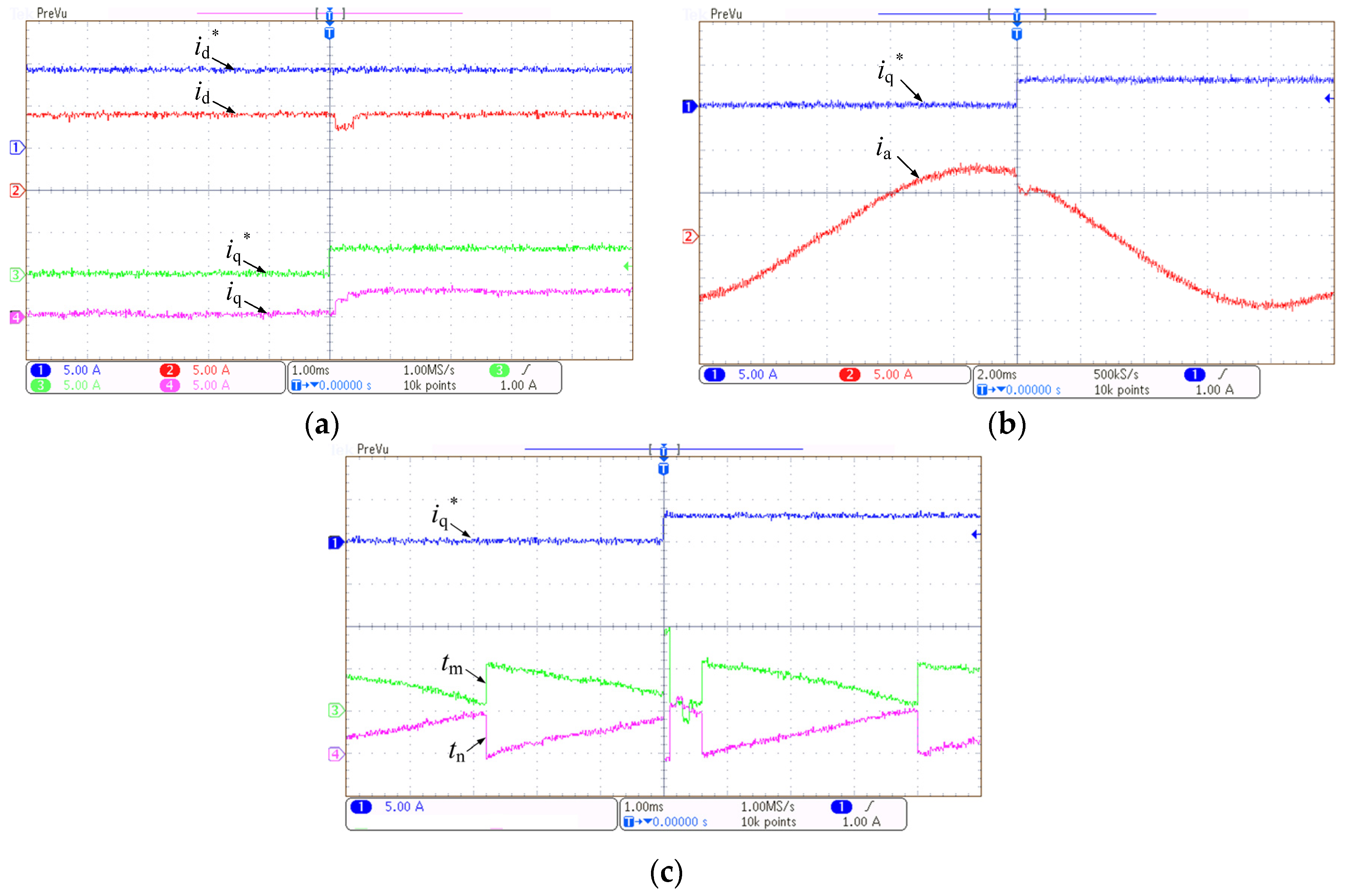
4.2. Transient Responses

For the purpose of further illustrating the superiority of Method II with regard to the transient responses, experimental studies were carried out. Figure 14 and Figure 15 present the experimental waveforms with Method I adopted. As pointed out previously, when the reference current is step changed, the conventional Method I will lead to incorrect selection of the voltage vector and negative duration time, which as a result, deteriorates the transient behaviours of the converter. As shown in Figure 14 and Figure 15, a slow transient response can be observed for both rectifier and inverter modes, and furthermore, the cross-coupling effect arises. The d-axis is significantly influenced by the step change of the q-axis current.
Figure 14. Experimental results: dq-axis currents and Phase A current with iq* step changed from 0 to 3 A (rectifier mode, Method I, id* = 9 A). (a) dq-axis currents; (b) Phase A current; (c) tm and tn (25 μs/division).
Energies 09 00041 g014
Figure 15. Experimental results: dq-axis currents and Phase A current with iq* step changed from 0 A to 3 A (inverter mode, Method I, id* = 0 A). (a) dq-axis currents; (b) tm and tn (25 μs/division).
Energies 09 00041 g015
With the aim of performance comparison, Figure 16 demonstrates the results when Method II is used and the converter is operating in rectifier mode. These figures were obtained under the same situation as those of Figure 14. By comparing Figure 14 and Figure 16, the improvements are evident with respect to dynamic responses. Highly dynamic behaviours can be expected with Method II. Actually, these excellent behaviours presented by Method II result from the improved switching patterns, which avoid the negative application times, as shown in Figure 16c,d. A similar conclusion can be made when system behaviours in the case of inverter mode were compared, as show in Figure 15 and Figure 17.
Figure 16. Experimental results: dq-axis currents and Phase A current with iq* step changed from 0 A to 3 A (rectifier mode, Method II, id* = 0 A). (a) dq-axis currents; (b) Phase A current; (c) selected voltage vectors; (d) tm and tn (25 μs/division).
Energies 09 00041 g016
Figure 17. Experimental results: dq-axis currents and Phase A current with iq* step changed from 0 A to 3 A (inverter mode, Method II, id* = 0 A). (a) dq-axis currents; (b) tm and tn (25 μs/division).
Energies 09 00041 g017
Besides, system transient behaviours with an outer DC-voltage control loop were also tested. Figure 18 demonstrates system transient responses when the converter was operating in rectifier mode and a disturbance was introduced to the resistance load of the DC-link. The control strategy for the DC-link voltage was the typical PI controller, which generated the reference signals for the d-axis current. Additionally, the q-axis current remained zero. As can be seen in the waveforms, the d-axis current can track the reference current in a good way, and the q-axis was not influenced by this transient process, demonstrating the decoupling performances of the proposed controller.
Figure 18. Experimental results: dq-axis currents and dc voltage with load disturbances (Method II; reference DC voltage: 445 V; offset voltage of DC voltage signal: 400 V).
Energies 09 00041 g018

5. Conclusions

When the predictive current control strategy is adopted, three-phase grid-tied converters can be flexibly regulated based on system behaviour prediction and cost function minimization. However, due to the adoption of conventional switching patterns, system performance deteriorations often take place under the conditions of both bidirectional power flows and transient situations. This paper analysed the switching patterns of three-phase grid-tied reversible converters under different conditions and investigated the predicted duration time of voltage vectors under bidirectional power flows, i.e., rectifier mode and inverter mode. A detailed analysis of switching patterns was further conducted. An enhanced predictive current control strategy with improved switching patterns was then proposed. According to the obtained experimental results, the system performances of three-phase grid-tied reversible converters were improved in terms of both steady-state and transient behaviours.

Acknowledgments

This work was supported by the National Science Foundation of China under Grants 51477113 and 51107084.

Author Contributions

Zhanfeng Song and Yanjun Tian contributed to experimental validations. Zhe Chen and Yanting Hu contributed to the result analysis.

Conflicts of Interest

The authors declare no conflict of interest.

References

  1. Vazquez, S.; Leon, J.I.; Franquelo, L.G.; Rodriguez, J.; Young, H.A.; Marquez, A.; Zanchetta, P. Model predictive control: A review of its applications in power electronics. IEEE Ind. Electron. Mag. 2014, 8, 16–31. [Google Scholar] [CrossRef] [Green Version]
  2. Min, R.; Chen, C.; Zhang, X.; Zou, X.; Tong, Q.; Zhang, Q. An optimal current observer for predictive current controlled buck DC-DC converters. Sensors 2014, 14, 8851–8868. [Google Scholar] [CrossRef] [PubMed]
  3. Tong, Q.; Chen, C.; Zhang, Q.; Zou, X. A sensorless predictive current controlled boost converter by using an EKF with load variation effect elimination function. Sensors 2015, 15, 9986–10003. [Google Scholar] [CrossRef] [PubMed]
  4. Zhang, Y.; Xie, W.; Li, Z.; Zhang, Y. Low-complexity model predictive power control: Double-vector-based approach. IEEE Trans. Ind. Electron. 2014, 61, 5871–5880. [Google Scholar] [CrossRef]
  5. Aguilera, R.P.; Quevedo, D.E.; Vazquez, S.; Franquelo, L.G. Generalized predictive direct power control for AC/DC converters. In Proceeding of the IEEE Annual International Energy Conversion Congress and Exhibition (ECCE Asia), Melbourne, VIC, Australia, 3–6 June 2013.
  6. Yaramasu, V.; Rivera, M.; Narimani, M.; Wu, B.; Rodriguez, J. Model predictive approach for a Simple and effective load voltage control of four-leg inverter with an output LC filter. IEEE Trans. Ind. Electron. 2014, 61, 5259–5270. [Google Scholar] [CrossRef]
  7. Riveros, J.A.; Barrero, F.; Levi, E.; Durán, M.J.; Toral, S.; Jones, M. Variable-speed five-phase induction motor drive based on predictive torque control. IEEE Trans. Ind. Electron. 2013, 60, 2957–2968. [Google Scholar] [CrossRef]
  8. Tarisciotti, L.; Zanchetta, P.; Watson, A.; Bifaretti, S.; Clare, J.C. Modulated model predictive control for a seven-level cascaded h-bridge back-to-back converter. IEEE Trans. Ind. Electron. 2014, 61, 5375–5383. [Google Scholar] [CrossRef]
  9. Zhang, Q.; Min, R.; Tong, Q.; Zou, X.; Liu, Z.; Shen, A. Sensorless predictive current controlled DC-DC converter with a self-correction differential current observer. IEEE Trans. Ind. Electron. 2014, 61, 6747–6757. [Google Scholar] [CrossRef]
  10. Tong, Q.; Zhang, Q.; Min, R.; Zou, X.; Liu, Z.; Chen, Z. Sensorless Predictive peak current control for boost converter using comprehensive compensation strategy. IEEE Trans. Ind. Electron. 2014, 61, 2754–2766. [Google Scholar] [CrossRef]
  11. Vu, T.; Chen, C.K.; Hung, C.W. A model predictive control approach for fuel economy improvement of a series hydraulic hybrid vehicle. Energies 2014, 7, 7017–7040. [Google Scholar] [CrossRef]
  12. Yang, J.; Zeng, Z.; Tang, Y.; Yan, J.; He, H.; Wu, Y. Load Frequency control in isolated micro-grids with electrical vehicles based on multivariable generalized predictive theory. Energies 2015, 8, 2145–2164. [Google Scholar] [CrossRef]
  13. Geyer, T.; Papafotiou, G.; Morari, M. Model predictive direct torque control—Part I: Concept, algorithm and analysis. IEEE Trans. Ind. Electron. 2009, 56, 1894–1905. [Google Scholar] [CrossRef]
  14. Papafotiou, G.; Kley, J.; Papdopoulos, K.; Bohren, P.; Morari, M. Model predictive direct torque control—Part II: Implementation and experimental evaluation. IEEE Trans. Ind. Electron. 2009, 56, 1906–1915. [Google Scholar] [CrossRef]
  15. Karamanakos, P.; Pavlou, K.; Manias, S. An enumeration-based model predictive control strategy for the cascaded H-bridge multilevel rectifier. IEEE Trans. Ind. Electron. 2014, 61, 3480–3489. [Google Scholar] [CrossRef]
  16. Choi, D.; Lee, K. Dynamic performance improvement of AC/DC converter using model predictive direct power control with finite control set. IEEE Trans. Ind. Electron. 2015, 62, 757–767. [Google Scholar] [CrossRef]
  17. Lim, C.; Levi, E.; Jones, M.; Rahim, N.A.; Hew, W. A fault-tolerant two-motor drive with FCS-MP-Based flux and torque control. IEEE Trans. Ind. Electron. 2014, 61, 6603–6614. [Google Scholar] [CrossRef]
  18. Ramírez, R.O.; Espinoza, J.R.; Villarroel, F.; Maurelia, E.; Reyes, M.E. A novel hybrid finite control set model predictive control scheme with reduced switching. IEEE Trans. Ind. Electron. 2014, 61, 5912–5920. [Google Scholar] [CrossRef]
  19. Davari, S.S.; Khaburi, D.; Kennel, R. An improved FCS–MPC algorithm for an induction motor with an imposed optimized weighting factor. IEEE Trans. Power Electron. 2012, 27, 1540–1551. [Google Scholar] [CrossRef]
  20. Calle-Prado, A.; Alepuz, S.; Bordonau, J.; Nicolas-Apruzzese, J.; Cortés, P.; Rodriguez, J. Model predictive current control of grid-connected neutral-point-clamped converters to meet low-voltage ride-through requirements. IEEE Trans. Ind. Electron. 2015, 62, 1503–1514. [Google Scholar] [CrossRef]
  21. Yaramasu, V.; Wu, B. Model predictive decoupled active and reactive power control for high-power grid-connected four-level diode-clamped inverters. IEEE Trans. Ind. Electron. 2014, 61, 3407–3416. [Google Scholar] [CrossRef]
  22. Yaramasu, V.; Wu, B.; Alepuz, S.; Kouro, S. Predictive control for low-voltage ride-through enhancement of three-level-boost and NPC-Converter-Based PMSG wind turbine. IEEE Trans. Ind. Electron. 2014, 61, 6832–6843. [Google Scholar] [CrossRef]
  23. Zhang, Z.; Xu, H.; Xue, M.; Chen, Z.; Sun, T.; Kennel, R.; Hackl, C.M. Predictive control with novel virtual-flux estimation for back-to-back power converters. IEEE Trans. Ind. Electron. 2015, 62, 2823–2834. [Google Scholar] [CrossRef]
  24. López, M.; Rodriguez, J.; Silva, C.; Rivera, M. Predictive torque control of a multidrive system fed by a dual indirect matrix converter. IEEE Trans. Ind. Electron. 2015, 62, 2731–2741. [Google Scholar] [CrossRef]
  25. Lim, C.; Levi, E.; Jones, M.; Rahim, N.A.; Hew, W. A comparative study of synchronous current control schemes based on FCS-MPC and PI-PWM for a two-motor three-phase drive. IEEE Trans. Ind. Electron. 2014, 61, 3867–3878. [Google Scholar] [CrossRef]
  26. Cortes, P.; Rodriguez, J.; Quevedo, D.E.; Silva, C. Predictive current control strategy with imposed load current spectrum. IEEE Trans. Power Electron. 2008, 23, 612–618. [Google Scholar] [CrossRef]
  27. Song, Z.; Xia, C.; Liu, T. Predictive current control of three-phase grid-connected converters with constant switching frequency for wind energy systems. IEEE Trans. Ind. Electron. 2013, 60, 2451–2464. [Google Scholar] [CrossRef]
  28. Xia, C.; Wang, M.; Song, Z.; Liu, T. Robust model predictive current control of three-phase voltage source PWM rectifier with online disturbance observation. IEEE Trans. Ind. Inf. 2012, 8, 459–471. [Google Scholar] [CrossRef]
  29. Vazquez, S.; Marquez, A.; Aguilera, R.; Quevedo, D.; Leon, J.I.; Franquelo, L.G. Predictive Optimal switching sequence direct power control for grid-connected power converters. IEEE Trans. Ind. Electron. 2015, 62, 2010–2020. [Google Scholar] [CrossRef]
  30. Song, Z.; Xia, C.; Liu, T.; Dong, N. A modified predictive control strategy of three-phase grid-connected converters with optimized action time sequence. Sci. China Technol. Sci. 2013, 56, 1017–1028. [Google Scholar] [CrossRef]
  31. Hu, J.; Zhu, Z. Investigation on switching patterns of direct power control strategies for grid-connected DC–AC converters based on power variation rates. IEEE Trans. Power Electron. 2011, 26, 3582–3598. [Google Scholar] [CrossRef]
  32. Song, Z.; Chen, W.; Xia, C. Predictive direct power control for three-phase grid-connected converters without sector information and voltage vector selection. IEEE Trans. Power Electron. 2014, 29, 5518–5531. [Google Scholar] [CrossRef]
  33. Sergio, A.; Rodriguez, M.A.; Oyarbide, E.; Torrealday, J.R. Predictive direct power control—A new control strategy for DC/AC converters. In Proceeding of the IECON 2006–32nd Annual Conference on IEEE Industrial Electronics, Paris, France, 6–10 November 2006; pp. 1661–1666.
  34. Larrinaga, S.A.; Vidal, M.A.R.; Oyarbide, E.; Apraiz, J.R.T. Predictive control strategy for DC/AC converters based on direct power control. Ind. Electron. IEEE Trans. 2007, 54, 1261–1271. [Google Scholar] [CrossRef]

