Reliability Analysis and Overload Capability Assessment of Oil-Immersed Power Transformers

Abstract

Smart grids have been constructed so as to guarantee the security and stability of the power grid in recent years. Power transformers are a most vital component in the complicated smart grid network. Any transformer failure can cause damage of the whole power system, within which the failures caused by overloading cannot be ignored. This research gives a new insight into overload capability assessment of transformers. The hot-spot temperature of the winding is the most critical factor in measuring the overload capacity of power transformers. Thus, the hot-spot temperature is calculated to obtain the duration running time of the power transformers under overloading conditions. Then the overloading probability is fitted with the mature and widely accepted Weibull probability density function. To guarantee the accuracy of this fitting, a new objective function is proposed to obtain the desired parameters in the Weibull distributions. In addition, ten different mutation scenarios are adopted in the differential evolutionary algorithm to optimize the parameter in the Weibull distribution. The final comprehensive overload capability of the power transformer is assessed by the duration running time as well as the overloading probability. Compared with the previous studies that take no account of the overloading probability, the assessment results obtained in this research are much more reliable.

1. Introduction

The power grid is an important infrastructure for a nation’s economic and social development, however, in recent years, the objective environment to guarantee the security and stability of the power grid is undergoing tremendous changes. Factors such as the rapid growth of the loads, the initial formation of the large area grid interconnection, as well as the influence of the global climate change all impact the electricity market and the effects on the power grid have become increasingly apparent, thus, guaranteeing the security and stability of the power grid represents a new challenge. To solve this problem, in recent years, smart grids have been constructed by comprehensively considering the market, safety, power quality and environmental factors. The term smart grid refers to a fully automated complicated power supply network, where each user and each node are monitored in real-time, to ensure a two-way flow of the current and information between the power plant and clients’ appliances. The features of the smart grid can be summarized as: self-healing, compatibility, interaction, coordination, efficiency, quality, and integration.

Power transformers is one of the most vital pieces of equipment in the smart grid. In addition, it is a network equipment whose structure is the most complex and sophisticated. Any failure in transformers can cause damage to the power system, among which failures caused by overloading cannot be ignored. The consequences of overloaded operation of power transformers can be serious. As indicated, when the current flow in the windings exceeds the rated current stated on the nameplate, i.e., the transformer operates under overload conditions, the load loss of transformers is proportional to the square of the current, conductor heating rises sharply, and the temperature of the windings and insulating oil surge accordingly. In this case, the transformer loss will increase due to the reason that power transformers are designed according to their rated capacity, so when the load of the transformer exceeds the rated capacity, the losses will increase. This will greatly affect the lifetime of the power transformer. In addition, transformers may fail due to the following two reasons: on the one hand, the transformer may be damaged since the overload operation would accelerate the cracking of insulating oil, generate bubbles, reduce the dielectric strength of the transformer, and cause an electrical breakdown. On the other hand, the excessive heat will reduce the mechanical strength of the windings, and when a short circuit occurs, coil deformation or mechanical instability will occur due to the external strong electric power. Therefore, overload capacity assessment is of particular importance in avoiding the catastrophic failure of power transformers and guaranteeing the normal operation of power grids.

Adequate and accurate assessment of power system reliability is a very challenging task that has been and still is under investigation. Previously developed power system reliability and security assessment models include the super components contingency model [1], the hybrid conditions-dependent outage model [2], and probability distribution based models such as the log-normal distribution [3] and the Weibull distribution [4]. As one of vital aspects in the power system reliability assessment, the overload capability of power transformers, has also been specifically surveyed by many researchers. For example, to make up the limitation of the American National Standards Instituteloading guide, which is only applicable to ambient temperatures above 0 °C, Aubin et al. [5] proposed a calculation method to assess the overload capacity of transformers for ambient temperatures below 0 °C. Tenbohlen et al. [6] developed on-line monitoring systems to assess the overload capacity of power transformers. Bosworth et al. [7] reported the development of electrochemical sensors for the measurement of phenol in transformer overloading evaluation. A stochastic differential equation was used by Edstrom et al. [8] to estimate the probability of transformer overloading. Estrada et al. [9] adopted magnetic flux entropy as a tool to predict transformer failures, and the overloading is just one aspect among the failures. Liu et al. [10] assessed the overload capacity of transformers through an online monitoring and overload factor calculated by a temperature reverse extrapolation approach. As known, when assessing network load capability, the hot-spot temperature is one the most significant factors. Thus, there are many studies devoted to hot-spot temperature forecasting such as the radial basis function network [11], a genetic algorithm based technique [12], and a local memory-based algorithm [13] provided by Galdi et al., the Takagi-Sugeno-Kang fuzzy model presented by Siano [14], the optimal linear combination of artificial neural network approach used by Pradhan and Ramu [15], the grey-box model introduced by Domenico et al. [16], etc. Though these researches make tremendous contributions, efforts on overload capability assessments should not be stopped, and new overload capability measurement techniques with respect to power transformers still need to be developed and exploited to improve the accuracy of overload capability assessment and provide more techniques to prevent failure of transformers caused by emergency overloads.

This research gives a new insight into how to measure the overload probability of oil-immersed power transformers. As known, the hot-spot temperature is the most critical factor in measuring the overload capability of power transformers. Thus, the hot-spot temperature is first calculated to measure the duration of running time under overload conditions. Then, the overloading probability is fitted by a mature and attractive Weibull distribution. Finally, the comprehensive overload capability of the power transformer is assessed from both the duration of running time under the overload conditions and the overloading probability aspects. This research is innovative in the following aspects: (a) apart from the duration of running time under the overload conditions, the overload capability is also assessed according to the overloading probability of the power transformer, which is measured by the Weibull distribution in this paper; (b) though the Weibull distribution is a quite mature and attractive method for fitting the distribution of data series, this paper improves the fitting performance of the Weibull distribution by proposing a new objective function to obtain the parameters in the Weibull distribution; (c) different from other researches, the shape parameter in the Weibull distribution in this paper is determined according to the mean of the shape parameter values obtained under ten different mutation scenarios in the differential evolutionary (DE) algorithms, i.e., the shape parameter is determined by taking results under different situations into account, this operation improves the accuracy of overload capability assessment further. The remainder of this paper is organized as follows: Section 2 introduces related techniques. Simulation results and discussions are presented in Section 3, while Section 4 concludes the whole research.

2. Related Techniques

2.1. Duration Running Time Calculation under Overloading Conditions

2.1.1. Steady-State Temperature Measurement

The final hot-spot temperature (${\mathsf{\theta }}_h$) of the winding for power transformer is calculated by [17]:

$${\mathsf{\theta }}_h={\mathsf{\theta }}_a+\Delta {\mathsf{\theta }}_{br}{\left[\frac{1+R{K}^2}{1+R}\right]}^x+2\left[\Delta {\mathsf{\theta }}_{imr}-\Delta {\mathsf{\theta }}_{br}\right]K^y+H{g}_r{K}^y$$

(1)

where θ_a is the air temperature (°C), Δθ_br is the temperature rise in bottom (K), Δθ_imr is the average winding temperature rise (K), R is the ratio between the load losses at the rated load and no-load losses, K is the load current per unit and y is the index of the winding.

For a forced-directed oil circulation and forced air circulation (ODAF) transformer, the oil flow in the windings is affected by the oil pump as well as the guide channel, the viscosity of the oil has little effect on the temperature change of the transformer, however, at this time, the temperature effect of the conductor resistance must be considered. Therefore, based on Equation (1), the final hot-spot temperature (${{\mathsf{\theta }}^{\prime }}_h$) of the winding for power transformer is corrected using [17]:

$${{\mathsf{\theta }}^{\prime }}_h={\mathsf{\theta }}_h+0.15({\mathsf{\theta }}_h-{\mathsf{\theta }}_{hr})$$

(2)

where θ_h is the final hot-spot temperature of the windings by not taking the effect of the conductor resistance into account and obtained by Equation (1), θ_hr is the hot-spot temperature under the rated operating conditions.

2.1.2. Transient Temperature Measurement

With the changes of the transformer load, the temperature of the transformer will change as well. It is found that the temperature rise stabilization time of the electric insulating oil, which is 1.5 h, is much longer than that of the conductor (usually 5–10 min). Thus the transient temperature is measured as follows:

$$\Delta {\mathsf{\theta }}_{bt}=\Delta {\mathsf{\theta }}_{bi}+(\Delta {\mathsf{\theta }}_{bu}-\Delta {\mathsf{\theta }}_{bi})(1-e^{-t/{\tau }_0})$$

(3)

where Δθ_bi is the initial bottom oil temperature rise, Δθ_bu is the bottom oil temperature rise of the applied load at the in the steady state, and τ₀ is the winding time constant.

Therefore, once the limit hot-spot temperature of the winding is determined, with the assistance of the thermal characterization parameters obtained in the factory test, and taking no account of the life lost, the overload capacity of the transformer can be calculated by Equations (1)–(3).

2.2. Overloading Probability Measurement

It is indicated that the relationship between the active power of the three-phase transformer and the current is as follows:

$$P=\sqrt{3}UI\cos \mathsf{\phi }$$

(4)

where P is the active power, U and I are the voltage and current respectively, and $\cos \mathsf{\phi }$ is called the power factor. Therefore, the probability value of the current located in the interval [I₁, I₂) is as equal as that of the active power located in the interval $[\sqrt{3}U{I}_1\cos \mathsf{\phi },\sqrt{3}U{I}_2\cos \mathsf{\phi })$. This inspires us to carry out the overloading probability measurement by means of the active power probability fitting results, in the situation that the current values are unknown whereas the active power values are observed.

The Weibull distribution is one of the most commonly used the loss of life distributions in the reliability research of single samples. Its main feature is that the difference of shape parameters can reflect various failure mechanisms. Numerous experimental results demonstrate that the life of components, equipment, and systems that cause the global function to stop running owing to the failure or breakdown in certain parts obey the Weibull distribution [18]. Moreover, according to Reference [19], the life of liquid insulation obeys a Gumbel distribution, while the lifetime of solid insulation follows a two-parameter distribution or lognormal distribution. Therefore, this paper applies a two-parameter Weibull distribution to research the life distribution features of hot-spot absolute temperature insulation samples. The statistical analysis of Weibull life data is based on the following three assumptions [20]:

A1:

In each different stress level, the loss of life of hot-spot absolute temperature insulation samples all obeys the Weibull distribution. That is to say, the distribution type of life will not change with increasing stress level.

A2:

In each different stress level, the failure mechanism of hot-spot absolute temperature insulation samples mush keep consistent. However, owing to the randomness of experimental data, the shape parameters of Weibull distribution can be only approximately equal.

A3:

The life of hot-spot absolute temperature insulation samples that obeys the Weibull distribution should the function of trial voltage and temperature. If A1 and A2 are satisfied, the hot-spot absolute temperature insulation samples obey the Weibull distribution. Assume that the main aim of A3 is to realize the data extrapolation.

The three assumptions are built based on certain physics, and we can use professional knowledge and engineering experience to judge whether they are true. In the statistical analysis, both hypothesis testing and correlation coefficient test can be applied to confirm their existence.

The active power distribution of the transformer is surveyed with the assistance of the Weibull distribution in this paper. The probability density function of the Weibull distribution can be described by:

$$f(a)=(\frac{k}{c}){(\frac{a}{c})}^{k-1}\exp \left[-{(\frac{a}{c})}^k\right]$$

(5)

where a is the active power with the unit of kW, k is the dimensionless shape parameter and c is the scale parameter with the same unit of the active power.

2.3. Objective Function

To obtain the unknown shape and scale parameters, in this research, a new objective function is constructed and the results obtained by this new objective function are compared with those obtained by two other frequently used objective functions.

2.3.1. The New Proposed Objective Function

According to the Probability Density Function (PDF) of the Weibull distribution, the expected value (E(a)) and the variance (Var(a)) of the active power can be obtained by:

$$E(a)=c\Gamma (1+\frac{1}{k})$$

(6)

and:

$$Var(a)=c^2\Gamma (1+\frac{2}{k})-c^2{\Gamma }^2(1+\frac{1}{k})$$

(7)

The new objective function constructed in this paper benefits from the following idea. As known, the mean square error (MSE) defined as follows is always been used as the objective function:

$$\mathrm{MSE}=\frac{1}{n}{\displaystyle \sum _{i=1}^n{(x_i-{\widehat{x}}_i)}^2}$$

(8)

where $x_i$ and ${\widehat{x}}_i$ are the observed and forecasted values, respectively. Let Y be a random variable and the possible values for Y are $y_1,y_2,\dots ,y_n$, where $y_i=x_i-{\widehat{x}}_i$. Then Equation (8) can be written as:

$$\mathrm{MSE}=\frac{1}{n}{\displaystyle \sum _{i=1}^n{y}_i^2}$$

(9)

which can be seen as:

$$\mathrm{MSE}=E(Y^2)$$

(10)

where E(Y²) represents the expected value of the variable Y². According to the following formula:

$$Var(Y)=E(Y^2)-{\left[E(Y)\right]}^2$$

(11)

Equation (10) is equivalent to:

$$\mathrm{MSE}={\left[E(Y)\right]}^2+Var(Y)$$

(12)

where E(Y) and Var(Y) denote the expected value and variance of the variable Y, respectively. Based on the calculation results obtained by Equations (6) and (7):

$${\left[E(a)\right]}^2+Var(a)=c^2\Gamma (1+\frac{2}{k})$$

(13)

However, there is always some error between the left side and the right side of the Equation (13). Thus, the residual value ε defined as below is used as the objective function:

$${\mathsf{\epsilon }}_1={\left[E(a)\right]}^2+Var(a)-c^2\Gamma (1+\frac{2}{k})$$

(14)

where E(a) represents the mean value of the active power and Var(a) denotes the variance of the active power. Then according to Equation (6), the scale parameter c can be obtained by:

$$c=\frac{E(a)}{\Gamma (1+1/k)}$$

(15)

So by substituting Equation (15) into Equation (14), the final objection function used to optimize the shape parameter k can be expressed as:

$${\mathsf{\epsilon }}_1={\left[E(a)\right]}^2+Var(a)-\frac{{\left[E(a)\right]}^2\Gamma (1+2/k)}{{\Gamma }^2(1+1/k)}$$

(16)

2.3.2. The First Comparison Objective Function

To verify the performance of the DE algorithm under different objective functions, the first objective function used to compare with the new one proposed in this paper is expressed as:

$${\mathsf{\epsilon }}_2=\frac{Var(a)}{{\left[E(a)\right]}^2}-\frac{\Gamma (1+2/k)-{\Gamma }^2(1+1/k)}{{\Gamma }^2(1+1/k)}$$

(17)

where E(a) represents the mean value of the active power and Var(a) denotes the variance of the active power. Similarly, Equation (17) is only used to optimize the shape parameter. The scale parameter in this comparison strategy is obtained by Equation (15) just as it did in the new proposed objective function. The construction of this objective function can be found in Appendix A.

2.3.3. The Second Comparison Objective Function

The second objective function, which used to compare with the new proposed one in this paper and is derived from the maximum likelihood estimation, can be expressed as:

$${\epsilon }_3=k-{\left[\frac{{\displaystyle {\sum }_{i=1}^n{a}_i^k\ln a_i}}{{\displaystyle {\sum }_{i=1}^n{a}_i^k}}-\frac{{\displaystyle {\sum }_{i=1}^n\ln a_i}}{n}\right]}^{1/k}$$

(18)

where n is the active power sample number and ${\left\{a_i\right\}}_{i=1}^n$ is the active power series of the transformer. The construction of this objective function can be found in Appendix B. Once the value of the shape parameter k has been obtained, the scale parameter c is determined according to:

$$c={(\frac{1}{n}{\displaystyle \sum _{i=1}^n{a}_i^k})}^{1/k}$$

(19)

2.4. Intelligent Optimization Algorithms

To obtain the optimum shape and scale parameters, the differential evolution (DE) algorithm is used in this research. The usage of the DE algorithm is built on the basis of the three previous described objective functions. In general, the DE algorithm contains three procedures: mutation, crossover and selection [21].

Procedure 1 (mutation): In this step, ten different mutation scenarios are employed in this research to survey the performance of the three objective functions. Given a population with N parameter vectors $X_i^G$, (i = 1, 2, 3, …, N for each generation G), these ten scenarios are expressed as follows:

$$\mathrm{Scenario\; 1}:v_i^{G+1}=x_{r1}^G+F\times (x_{r2}^G-x_{r3}^G),r1\ne r2\ne r3\ne i;$$

(20)

$$\mathrm{Scenario\; 2}:v_i^{G+1}=x_i^G+F_1\times (x_{best}^G-x_i^G)+F_2\times (x_{r2}^G-x_{r3}^G);$$

(21)

$$\mathrm{Scenario\; 3}:v_i^{G+1}=x_{best}^G+(x_{r1}^G-x_{r2}^G)\times ((1-0.9999)\times rand+F);$$

(22)

$$\mathrm{Scenario\; 4}:v_i^{G+1}=x_{r1}^G+F_1\times (x_{r2}^G-x_{r3}^G),F_1=(1-F)\times rand+F;$$

(23)

where the values of F₁ are the same for all of the parameters need to be estimated.

$$\mathrm{Scenario\; 5}:v_i^{G+1}=x_{r1}^G+F_1\times (x_{r2}^G-x_{r3}^G),F_1=(1-F)\times rand+F;$$

(24)

$$\mathrm{Scenario\; 6}:v_i^{G+1}=x_i^G+F\times (x_{r2}^G-x_{r3}^G);$$

(25)

$$\mathrm{Scenario\; 7}:v_i^{G+1}=x_{r1}^G+F\times (x_{r2}^G-x_{r3}^G+x_{r4}^G-x_{r5}^G);$$

(26)

$$\mathrm{Scenario\; 8}:v_i^{G+1}=x_i^G+F\times (x_{r2}^G-x_{r3}^G+x_{r4}^G-x_{r5}^G);$$

(27)

$$\mathrm{Scenario\; 9}:v_i^{G+1}=x_i^G+F\times (x_{best}^G-x_i^G)+0.5\times (x_{r2}^G-x_{r3}^G);$$

(28)

$$\mathrm{Scenario\; 10}:v_i^{G+1}=\{\begin{array}{l}{x}_{r1}^G+F\times (x_{r2}^G-x_{r3}^G),\begin{array}{}\end{array}\mathrm{if}\begin{array}{}\end{array}rand<0.5\hfill \\ x_{r1}^G+0.5\times (F+1)\times (x_{r1}^G+x_{r2}^G-2\times x_{r3}^G),\begin{array}{}\end{array}\mathrm{if}\begin{array}{}\end{array}rand\ge 0.5\hfill \end{array}$$

(29)

where r1, r2, r3, r4, r5 are integer numbers randomly selected from {1, 2, …, N}, F is the mutation factor chosen from the range [0, 1], and $x_i^G$ and $x_{best}^G$ are the ith and the best individuals in generation G, respectively.

Procedure 2 (Crossover): The exponential crossover approach is employed in this step. Component update in the trial vector $U_i^{G+1}=(u_{1i}^{G+1},u_{2i}^{G+1},\dots ,u_{Di}^{G+1})$ is described as:

$$u_{ji}^{G+1}=\{\begin{array}{ll}{v}_{{}_{ji}}^{G+1},\hfill & \mathrm{if}j\in \left\{k,{\langle k+1\rangle }_n,\dots ,{\langle k+L-1\rangle }_n\right\}\\ x_{ji}^G,\hfill & \text{otherwise}\end{array},j=1,2,\dots D$$

(30)

where k and L are random values selected from the set {1, 2, …, n}, and 〈j〉_n is set to j in the case of j ≤ n while j − n in the case of j > n.

Procedure 3 (Selection): This step is operated according to the following law:

$$X_i^{G+1}=\{\begin{array}{ll}{U}_i^{G+1},\hfill & \mathrm{if}f(U_i^{G+1})\le f(X_i^G)\\ X_i^G,\hfill & \text{otherwise}\end{array}$$

(31)

The DE algorithm is terminated in the case of the value of ε or the iteration number reaches the expected level.

2.5. New Proposed Overloading Probability Measurement Algorithm

Based on the above related techniques, a new proposed overloading probability measurement algorithm is proposed, the outline of this algorithm is shown in Algorithm 1.

Algorithm 1 New proposed overloading probability measurement algorithm

Input: Active power a—a sequence of sample data

Output: The probability density function of the active power

1. Initialize the shape parameter k

2.  WHILE ( ε > predefined error level) DO

3. Update the shape parameter k with the DE algorithm

4. Calculate $\epsilon ={\left[E(a)\right]}^2+Var(a)-{\left[E(a)\right]}^2\Gamma (1+2/k)/{\Gamma }^2(1+1/k)$ by using the new obtained k

5.  END WHILE

6. Calculate $c=E(a)/\Gamma (1+1/k)$ by using the final value of k

7.  $f(a)=(k/c){(a/c)}^{k-1}\exp \left[-{(a/c)}^k\right]$

8.  RETURN f

2.6. Fitting Performance Evaluation Criteria

In this paper, two error evaluation criteria named the Kolmogorov-Smirnov test error (KSE) [22] and the root mean square error (RMSE) [23], are applied to the further comparison among the new proposed and the comparison objective functions. The related definitions are as follows:

$$\text{KSE=max}\left|S(a)-O(a)\right|$$

(32)

$$\text{RMSE=}{\left[\frac{1}{n}{\displaystyle \sum _{i=1}^n{(a_{oi}-a_{ci})}^2}\right]}^{1/2}$$

(33)

where S(a) and O(a) are the Cumulative Distribution Function (CDF)values of the active power not exceeding a obtained by the selected function and by the actual data, respectively, ${\left\{a_{oi}\right\}}_{i=1}^n$ and ${\left\{a_{ci}\right\}}_{i=1}^n$ are the probability data series obtained by the observed data and the selected probability density function respectively, $n$ represents the number of the data.

3. Results and Discussion

In this paper, the overload capability of oil-immersed power transformers is assessed by the data sampled from three residential areas named Lake Neighborhood, North Neighborhood and Sunshine Mediterranean Neighborhood. The three-phase transformer used in the first residential area is a model S11-M-200/10 (HengAnYuan, Beijing, China), and those in the other two residential areas are both S11-M-400/10 units (HengAnYuan, Beijing, China), i.e. the rated capacity values of the transformers used in these three neighborhoods are 200, 400 and 400 kVA, respectively.

3.1. Overloading Probability Fitting Results

The DE algorithm is carried out and terminated when the objective function is no larger than 1 × 10⁻⁵ in this paper. Table 1 presents performance of the three objective functions by using different DE mutation scenarios in terms of the iteration number and the actual obtained objective function values when the termination condition is reached. For convenience, the new proposed objective function, the first comparison objective function and the second objective function are named the objective function 1, the objective function 2 and the objective function 3 in Table 1, respectively.

As seen from Table 1, when the new proposed objective function is applied to the shape parameter optimization, the iteration numbers of the DE algorithm needed to reach the objective function level are smaller than those obtained by the other two comparison objective functions under most of the mutation scenarios. For the Lake Neighborhood, the percentages by which the new proposed objective function outperforms the first comparison and the second comparison objective functions from the iteration numbers are 30% and 100%, respectively. For the North Neighborhood, these corresponding two values are 70% and 90%, respectively, while for the Sunshine Mediterranean Neighborhood, the values are both 100%. Note that in the case where the two objective functions have the same iteration numbers, the superior one is further selected by the actual obtained objective function values.

Furthermore, the shape parameter values obtained by the new proposed objective function is much closer to those obtained by the first comparison objective function. Since the iteration numbers need to reach the objective function level of the first comparison objective function are smaller than those obtained by the second comparison objective function, the first comparison objective function can be regarded as a better one as compared to the second comparison objective function from the iteration speed perspective. According to this, it can be concluded that the new proposed objective function is the best one among the three objective functions from the iteration speed perspective.

It can also be observed from Table 1 that the new proposed objective function is more sensitive to the change of the mutation scenarios as compared to the other two objective functions. This can be indicated by the ten shape parameter values under ten different mutation scenarios in the Sunshine Mediterranean Neighborhood, where those obtained by the new proposed objective function varied (though the variation is small) with the change of the mutation scenarios, while there are almost no change to the shape parameters obtained by the other two objective functions under different mutation scenarios). Thus, the new proposed objective function is better for its sensitivity.

As shown in Table 1, there is little difference among the shape parameter values obtained by the first objective function under the ten different mutation scenarios. Thus, to avoid the one-sidedness, the final shape parameter in this paper is determined by calculating the mean of the ten shape parameter values. As also seen from Table 1, the shape parameter values obtained by the new proposed and the first comparison objective functions are nearly equal. However, results obtained by the second comparison objective functions have larger difference as those gained by the new proposed objective functions. In the next section, this conclusion will be convinced by some statistics analysis and a test named the Moses Extreme Reactions (MER).

Table 1. Parameters obtained by three different objective functions.

Lake Neighborhood					North Neighborhood					Sunshine Mediterranean Neighborhood
Objective Function Type	Mutation Scenario	Iteration Number	Objective Function Value	k	Objective Function Type	Mutation Scenario	Iteration Number	Objective Function Value	k	Objective Function Type	Mutation Scenario	Iteration Number	Objective Function Value	k
1	1	18	$6.9259\times {10}^{-6}$	1.7718	1	1	18	$2.4220\times {10}^{-6}$	1.4420	1	1	13	$3.8005\times {10}^{-6}$	1.5006
	2	13	$9.2435\times {10}^{-6}$	1.7718		2	11	$8.9312\times {10}^{-6}$	1.4420		2	4	$6.9169\times {10}^{-6}$	1.5001
	3	10	$7.4746\times {10}^{-6}$	1.7718		3	11	$3.8947\times {10}^{-6}$	1.4420		3	6	$5.8058\times {10}^{-6}$	1.5002
	4	16	$6.9762\times {10}^{-6}$	1.7718		4	20	$3.9435\times {10}^{-6}$	1.4420		4	11	$6.5550\times {10}^{-7}$	1.5004
	5	20	$5.6428\times {10}^{-6}$	1.7718		5	19	$3.2357\times {10}^{-6}$	1.4420		5	14	$9.6016\times {10}^{-6}$	1.5008
	6	19	$9.4087\times {10}^{-6}$	1.7718		6	25	$9.9202\times {10}^{-6}$	1.4420		6	23	$4.2009\times {10}^{-7}$	1.5004
	7	17	$4.6030\times {10}^{-6}$	1.7718		7	19	$6.2421\times {10}^{-6}$	1.4420		7	9	$4.0648\times {10}^{-6}$	1.5006
	8	34	$4.9812\times {10}^{-6}$	1.7718		8	39	$7.1700\times {10}^{-6}$	1.4420		8	7	$2.6037\times {10}^{-6}$	1.5005
	9	13	$7.4412\times {10}^{-6}$	1.7718		9	12	$2.0244\times {10}^{-6}$	1.4420		9	7	$6.3303\times {10}^{-6}$	1.5007
	10	13	$9.7352\times {10}^{-6}$	1.7718		10	16	$7.5910\times {10}^{-7}$	1.4420		10	12	$5.6289\times {10}^{-6}$	1.5002
2	1	16	$8.3027\times {10}^{-7}$	1.7718	2	1	18	$8.4671\times {10}^{-6}$	1.4420	2	1	16	$8.7020\times {10}^{-8}$	1.5004
	2	13	$5.9090\times {10}^{-6}$	1.7718		2	14	$7.8769\times {10}^{-7}$	1.4420		2	13	$4.4437\times {10}^{-6}$	1.5004
	3	12	$1.6624\times {10}^{-6}$	1.7718		3	12	$8.9997\times {10}^{-7}$	1.4420		3	10	$8.0433\times {10}^{-6}$	1.5004
	4	14	$1.8828\times {10}^{-6}$	1.7718		4	19	$3.1183\times {10}^{-6}$	1.4420		4	24	$1.1569\times {10}^{-6}$	1.5004
	5	12	$8.6969\times {10}^{-6}$	1.7718		5	18	$5.0858\times {10}^{-6}$	1.4420		5	19	$1.5519\times {10}^{-6}$	1.5004
	6	23	$7.7303\times {10}^{-6}$	1.7718		6	38	$6.8227\times {10}^{-6}$	1.4420		6	37	$8.6291\times {10}^{-6}$	1.5004
	7	14	$5.2478\times {10}^{-6}$	1.7718		7	19	$5.2558\times {10}^{-6}$	1.4420		7	12	$7.9567\times {10}^{-6}$	1.5004
	8	36	$7.3341\times {10}^{-6}$	1.7718		8	40	$3.7643\times {10}^{-6}$	1.4420		8	26	$8.7335\times {10}^{-6}$	1.5004
	9	6	$2.7901\times {10}^{-6}$	1.7718		9	17	$5.2971\times {10}^{-6}$	1.4420		9	12	$3.3013\times {10}^{-6}$	1.5004
	10	13	$3.3655\times {10}^{-6}$	1.7718		10	18	$1.6249\times {10}^{-6}$	1.4420		10	15	$3.0078\times {10}^{-6}$	1.5004
3	1	21	$5.5706\times {10}^{-6}$	1.8322	3	1	21	$3.4492\times {10}^{-6}$	1.5010	3	1	21	$9.1215\times {10}^{-6}$	1.5743
	2	16	$6.0681\times {10}^{-6}$	1.8322		2	13	$8.2479\times {10}^{-6}$	1.5010		2	13	$9.8864\times {10}^{-7}$	1.5743
	3	15	$2.6695\times {10}^{-6}$	1.8322		3	10	$5.9725\times {10}^{-6}$	1.5010		3	13	$7.4311\times {10}^{-6}$	1.5743
	4	19	$8.4953\times {10}^{-6}$	1.8322		4	23	$6.4584\times {10}^{-6}$	1.5010		4	23	$5.0605\times {10}^{-8}$	1.5743
	5	23	$2.9226\times {10}^{-6}$	1.8322		5	22	$1.7365\times {10}^{-6}$	1.5010		5	19	$1.0723\times {10}^{-6}$	1.5743
	6	50	$2.9237\times {10}^{-6}$	1.8322		6	39	$7.8088\times {10}^{-6}$	1.5010		6	42	$4.8807\times {10}^{-6}$	1.5743
	7	26	$1.4879\times {10}^{-6}$	1.8322		7	24	$7.5942\times {10}^{-6}$	1.5010		7	18	$3.6736\times {10}^{-6}$	1.5743
	8	43	$4.7320\times {10}^{-6}$	1.8322		8	44	$2.3022\times {10}^{-6}$	1.5010		8	50	$8.4293\times {10}^{-6}$	1.5743
	9	16	$9.1194\times {10}^{-6}$	1.8322		9	16	$4.8699\times {10}^{-7}$	1.5010		9	15	$9.2910\times {10}^{-6}$	1.5743
	10	18	$8.8692\times {10}^{-6}$	1.8322		10	16	$4.7118\times {10}^{-6}$	1.5010		10	24	$3.0137\times {10}^{-6}$	1.5743

Table 1. Parameters obtained by three different objective functions.

Lake Neighborhood					North Neighborhood					Sunshine Mediterranean Neighborhood
Objective Function Type	Mutation Scenario	Iteration Number	Objective Function Value	k	Objective Function Type	Mutation Scenario	Iteration Number	Objective Function Value	k	Objective Function Type	Mutation Scenario	Iteration Number	Objective Function Value	k
1	1	18	$6.9259\times {10}^{-6}$	1.7718	1	1	18	$2.4220\times {10}^{-6}$	1.4420	1	1	13	$3.8005\times {10}^{-6}$	1.5006
	2	13	$9.2435\times {10}^{-6}$	1.7718		2	11	$8.9312\times {10}^{-6}$	1.4420		2	4	$6.9169\times {10}^{-6}$	1.5001
	3	10	$7.4746\times {10}^{-6}$	1.7718		3	11	$3.8947\times {10}^{-6}$	1.4420		3	6	$5.8058\times {10}^{-6}$	1.5002
	4	16	$6.9762\times {10}^{-6}$	1.7718		4	20	$3.9435\times {10}^{-6}$	1.4420		4	11	$6.5550\times {10}^{-7}$	1.5004
	5	20	$5.6428\times {10}^{-6}$	1.7718		5	19	$3.2357\times {10}^{-6}$	1.4420		5	14	$9.6016\times {10}^{-6}$	1.5008
	6	19	$9.4087\times {10}^{-6}$	1.7718		6	25	$9.9202\times {10}^{-6}$	1.4420		6	23	$4.2009\times {10}^{-7}$	1.5004
	7	17	$4.6030\times {10}^{-6}$	1.7718		7	19	$6.2421\times {10}^{-6}$	1.4420		7	9	$4.0648\times {10}^{-6}$	1.5006
	8	34	$4.9812\times {10}^{-6}$	1.7718		8	39	$7.1700\times {10}^{-6}$	1.4420		8	7	$2.6037\times {10}^{-6}$	1.5005
	9	13	$7.4412\times {10}^{-6}$	1.7718		9	12	$2.0244\times {10}^{-6}$	1.4420		9	7	$6.3303\times {10}^{-6}$	1.5007
	10	13	$9.7352\times {10}^{-6}$	1.7718		10	16	$7.5910\times {10}^{-7}$	1.4420		10	12	$5.6289\times {10}^{-6}$	1.5002
2	1	16	$8.3027\times {10}^{-7}$	1.7718	2	1	18	$8.4671\times {10}^{-6}$	1.4420	2	1	16	$8.7020\times {10}^{-8}$	1.5004
	2	13	$5.9090\times {10}^{-6}$	1.7718		2	14	$7.8769\times {10}^{-7}$	1.4420		2	13	$4.4437\times {10}^{-6}$	1.5004
	3	12	$1.6624\times {10}^{-6}$	1.7718		3	12	$8.9997\times {10}^{-7}$	1.4420		3	10	$8.0433\times {10}^{-6}$	1.5004
	4	14	$1.8828\times {10}^{-6}$	1.7718		4	19	$3.1183\times {10}^{-6}$	1.4420		4	24	$1.1569\times {10}^{-6}$	1.5004
	5	12	$8.6969\times {10}^{-6}$	1.7718		5	18	$5.0858\times {10}^{-6}$	1.4420		5	19	$1.5519\times {10}^{-6}$	1.5004
	6	23	$7.7303\times {10}^{-6}$	1.7718		6	38	$6.8227\times {10}^{-6}$	1.4420		6	37	$8.6291\times {10}^{-6}$	1.5004
	7	14	$5.2478\times {10}^{-6}$	1.7718		7	19	$5.2558\times {10}^{-6}$	1.4420		7	12	$7.9567\times {10}^{-6}$	1.5004
	8	36	$7.3341\times {10}^{-6}$	1.7718		8	40	$3.7643\times {10}^{-6}$	1.4420		8	26	$8.7335\times {10}^{-6}$	1.5004
	9	6	$2.7901\times {10}^{-6}$	1.7718		9	17	$5.2971\times {10}^{-6}$	1.4420		9	12	$3.3013\times {10}^{-6}$	1.5004
	10	13	$3.3655\times {10}^{-6}$	1.7718		10	18	$1.6249\times {10}^{-6}$	1.4420		10	15	$3.0078\times {10}^{-6}$	1.5004
3	1	21	$5.5706\times {10}^{-6}$	1.8322	3	1	21	$3.4492\times {10}^{-6}$	1.5010	3	1	21	$9.1215\times {10}^{-6}$	1.5743
	2	16	$6.0681\times {10}^{-6}$	1.8322		2	13	$8.2479\times {10}^{-6}$	1.5010		2	13	$9.8864\times {10}^{-7}$	1.5743
	3	15	$2.6695\times {10}^{-6}$	1.8322		3	10	$5.9725\times {10}^{-6}$	1.5010		3	13	$7.4311\times {10}^{-6}$	1.5743
	4	19	$8.4953\times {10}^{-6}$	1.8322		4	23	$6.4584\times {10}^{-6}$	1.5010		4	23	$5.0605\times {10}^{-8}$	1.5743
	5	23	$2.9226\times {10}^{-6}$	1.8322		5	22	$1.7365\times {10}^{-6}$	1.5010		5	19	$1.0723\times {10}^{-6}$	1.5743
	6	50	$2.9237\times {10}^{-6}$	1.8322		6	39	$7.8088\times {10}^{-6}$	1.5010		6	42	$4.8807\times {10}^{-6}$	1.5743
	7	26	$1.4879\times {10}^{-6}$	1.8322		7	24	$7.5942\times {10}^{-6}$	1.5010		7	18	$3.6736\times {10}^{-6}$	1.5743
	8	43	$4.7320\times {10}^{-6}$	1.8322		8	44	$2.3022\times {10}^{-6}$	1.5010		8	50	$8.4293\times {10}^{-6}$	1.5743
	9	16	$9.1194\times {10}^{-6}$	1.8322		9	16	$4.8699\times {10}^{-7}$	1.5010		9	15	$9.2910\times {10}^{-6}$	1.5743
	10	18	$8.8692\times {10}^{-6}$	1.8322		10	16	$4.7118\times {10}^{-6}$	1.5010		10	24	$3.0137\times {10}^{-6}$	1.5743

3.2. Three Objective Functions Comparison

In this section, the three objective functions are compared from the iteration number and the objective function value aspects. These three objective functions are firstly analyzed by comparing the corresponding results with regard to the three groups and two group pairs shown in Figure 1.

Figure 1. Groups and group pairs.

Figure 1. Groups and group pairs.

3.2.1. Analysis and Comparison Over the Three Groups

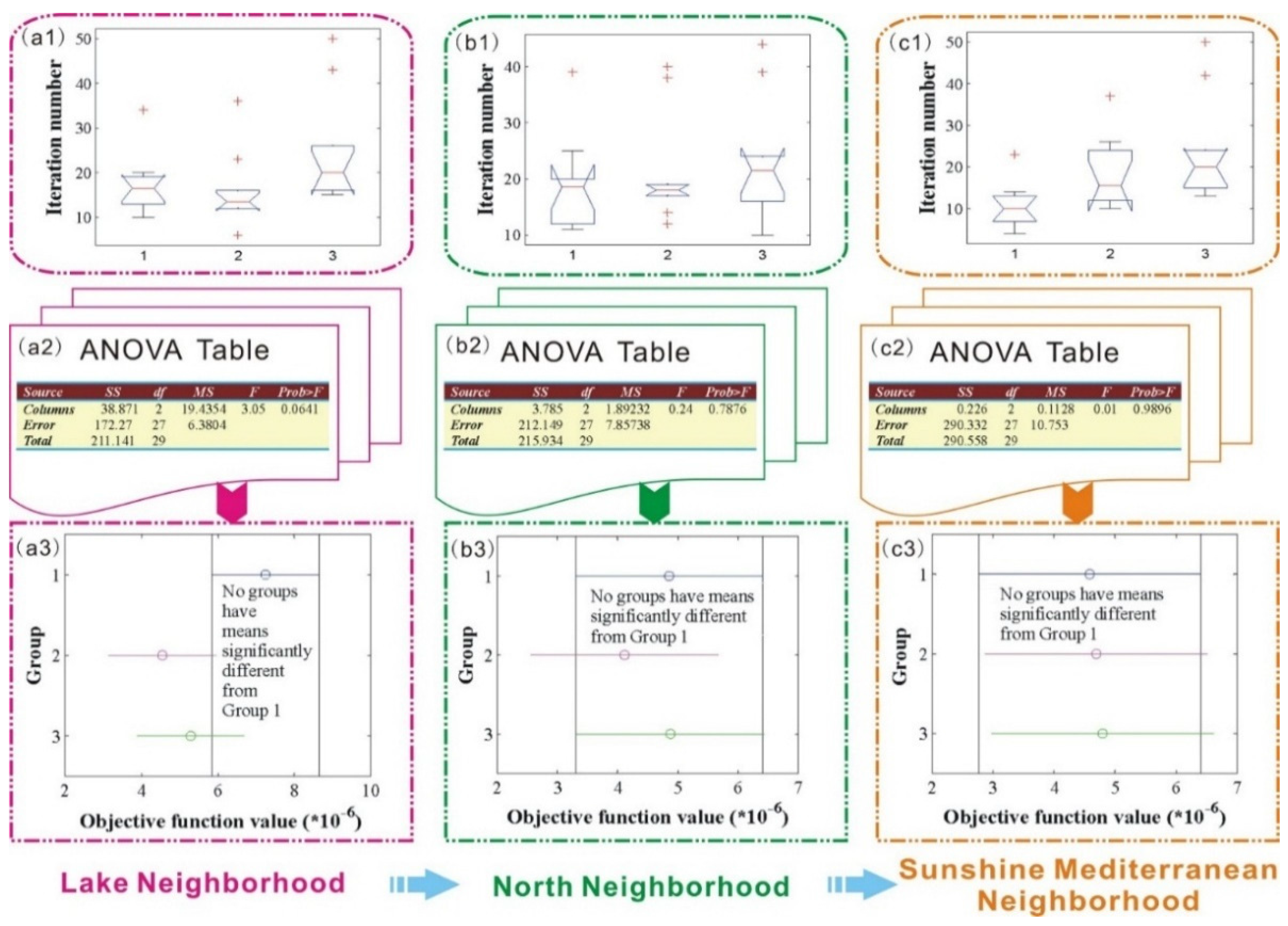
Boxplot Results Analysis

Figure 2(a1–c1) show the boxplots of the iteration number over the above defined three groups, where on each box, the central mark is the median, and the edges of the box are the lower quantile and the upper quantile, respectively. The lower quantile, the median and the upper quantile means the 0.25, 0.5 and 0.75 quantiles, respectively, where the f quantile corresponding to a datum q(f) means that below this datum, approximately a decimal fraction f of the data can be found. It is calculated in this way: Sorting the data in a sequence ${\left\{x_j\right\}}_{j=1,2,\dots ,n}$ in an ascending order. By this, the sorted data ${\left\{x_{\langle i\rangle }\right\}}_{i=1,2,\dots ,n}$ have rank i = 1, 2, …, n. Then the quantile value f_i for the datum x_〈i〉 (equal to q(f_i)) is computed as:

$$f_i=\frac{i-0.5}{n},i=1,2,\dots ,n$$

(34)

While in the case of the desired quantile value f is equal to none of the f_i values shown in Equation (34), the f quantile q(f) is found by linear interpolation, i.e.:

$$q(f)=q(f_1)+\frac{f-f_1}{f_2-f_1}\left[q(f_2)-q(f_1)\right]$$

(35)

where f₁ and f₂ are two unequal values selected from {0.5/n, 1.5/n, …, (n − 0.5)/n}. Note that in the case of the probability value f is less than 0.5)/n, the value q(f) is assigned to the first value x_〈1〉, while the value q(f) is assigned to the last value x_〈n〉, when the probability value f is greater than (n − 0.5)/n.

In addition, Figure 2(a1–c1) also show the outliers beyond the whiskers which are displayed using +. The whiskers in this paper are specified as 1.0 times the interquartile range, i.e., points larger than q(0.75) + w[q(0.75) − q(0.25)] or smaller than q(0.25) − w[q(0.75) − q(0.25)] are defined as outliers, where w is set to 1.0 in this paper.

Figure 2. Boxplot and ANOVA comparison results of the three objective functions.

Figure 2. Boxplot and ANOVA comparison results of the three objective functions.

As seen from Figure 2(a1–c1), for the Lake Neighborhood, the number of outliers in the three groups are 1, 3, 2, respectively, while for the other two Neighborhoods, the number of outliers in Groups 1 and 3remains the same, while values in Group 2 turns to 4 and 1 for the North Neighborhood and the Sunshine Mediterranean Neighborhood, respectively.

Analysis of Variance

Next one-way analysis of variance (ANOVA) was conducted to compare the objective function results of the three groups. Figure 2(a2–c2) provide the ANOVA results of the three neighborhoods, respectively, where SS, df, MS represent the sum of squares, degree of freedom and mean square, respectively, and Columns, Error mean the feature between groups and feature within groups, respectively, and Total indicates the sum of the Columns and the Error. Specifically, we have the following definitions:

$$SS\text{\hspace{0.17em}of\hspace{0.17em}the\hspace{0.17em}}Columns={\displaystyle \sum _{i=1}^k{n}_i{({\overline{x}}_i-\overline{x})}^2}$$

(36)

$$SS\text{\hspace{0.17em}of\hspace{0.17em}the\hspace{0.17em}}Error={\displaystyle \sum _{i=1}^k{\displaystyle \sum _{j=1}^{n_i}{(x_{ij}-{\overline{x}}_i)}^2}}$$

(37)

and

$$SS\text{\hspace{0.17em}of\hspace{0.17em}the\hspace{0.17em}}Total={\displaystyle \sum _{i=1}^k{\displaystyle \sum _{j=1}^{n_i}{(x_{ij}-\overline{x})}^2}}$$

(38)

where k is the number of the groups, x_ij denotes the jth sample in the ith group, n_i represents the number of the samples in the $i$ th group, and ${\overline{x}}_i$ and $\overline{x}$ indicates the mean of the samples in the ith group and the mean of the samples in all of the groups, respectively. The one-way ANOVA can be conducted according to the following four steps:

Step 1: Determine the null hypothesis. The null hypothesis of the one-way ANOVA is that samples in all of the groups are drawn from populations with the same mean.

Step 2: Select the test statistic. The test statistic of the one-way ANOVA used is the F statistic, which is defined as:

$$F=\frac{SS\text{\hspace{0.17em}of\hspace{0.17em}the\hspace{0.17em}}Columns/(k-1)}{SS\text{\hspace{0.17em}of\hspace{0.17em}the\hspace{0.17em}}Error/(n-k)}$$

(39)

where n is the total number of the samples, and k–1 and n–k are the degree of freedom of the SS of the Columns and SS of the Error, respectively.

Step 3: Calculate the value of the test statistic as well as the corresponding probability value p.

Step 4: Make decisions according to the significance level α. In the case of p < α, the null hypothesis should be rejected, and the decision that samples in all of the groups are not drawn from populations with the same mean is made; Otherwise, the null hypothesis should be accepted to demonstrate that samples in all of the groups are drawn from populations with the same mean.

As shown in Figure 2(a2–c2), all of the p values in the three neighborhoods are larger than the significance level α, which is set to 0.05 in this paper, this phenomenon indicates that for all of the three neighborhoods, the objective function samples in Groups 1–3 are drawn from populations with the same mean, Figure 2(a3–c3) display the mean comparison results of the three groups.

3.2.2. Test Over the Two Group Pairs

In this section, the three objective functions are analyzed by conducting the MER test over the two group pairs. The basic idea of the MER is that one group of the samples is regarded as the control group, while the other group of the samples is treated as the experimental group, then it is tested whether there are extreme reactions in the experimental group as compared to the control one. The conclusion of the MER is obtained by testing which one of the following hypothesis is accepted:

Null hypothesis: there is no significant difference between the distributions of samples in the control group and the experimental group; vs. Alternative hypothesis: there is significant difference between the distributions of samples in the control group and the experimental group.

If the experimental group has extreme reactions, it is assumed that there is no significant difference between the distributions of the control group and the experimental group; instead, there is significant difference between the distributions of these two groups. The detailed analysis process is as follows:

• First of all, samples in the two groups are mixed and ordered by ascending;
• Calculate the minimum rank R_min and the maximum rank R_max of the control group, and obtain the span by:

  $$S=R_{\max }-R_{\min }+1$$
• To eliminate the effect of the extreme values of the sample data on the analysis results, a proportional (usually this value is set to 5%) of the samples close to the left and the right ends are removed from the control group, and the span of the remaining samples which is named the trimmed span is calculated.

The MERs focus on the analysis of the span and the trimmed span. Obviously, if the values of the span or the trimmed span are small, the two sample groups cannot be mixed fully, and sample values in one group are greater than those in the other group, therefore, it can be regarded that as compared to the control group, the experimental group contains the extreme reactions, and thus the conclusion that there is significant difference between the distributions of these two groups can be obtained; otherwise, if the values of the span or the trimmed span are great, the two sample groups are mixed fully, and the phenomenon that sample values in one group are greater than those in the other group does not exist, therefore, it can be regarded that as compared to the control group, the experimental group does not contain extreme reactions, and thus the conclusion that there is no significant difference between the distributions of these two groups is reached. In general, the H statistics defined as below is used to evaluate the span or the trimmed span:

$$H={\displaystyle \sum _{i=1}^m{(R_i-\overline{R})}^2}$$

where m is the number of the samples in the control group, R_i is the rank of the ith control sample in the mixed samples, $\overline{R}$ is the average rank of the control samples. It can be proved that for small samples, the H statistics obey the Hollander distribution, while for large samples, the H statistics approximately obey a normal distribution.

If the value of p is smaller than the given confidence level α, then the null hypothesis should be rejected, and it is regarded that there is significant difference between the distributions of samples in the control group and the experimental group; otherwise, the null hypothesis should be accepted, and the conclusion that there is no significant difference between the distributions of samples in the control group and the experimental group can be obtained. In this paper, the MER technique is used to compare the difference of the three objective functions furthermore. Section 3.2.1 analyzed the three objective function mainly from the shape parameter aspect, in this section, the three objective functions will be analyzed through the iteration number as well as the objective function value.

Table 2 lists the descriptive statistics of Pair 1 and Pair 2, where N denotes the number of the samples in the pair and the hth percentile is equivalent to the h/100 quantile. As seen from Table 2, apart from the objective function value of the Lake Neighborhood, the standard deviation of which in Pair 2 is smaller than the one in Pair 1, for other items, the standard deviation values in Pair 2 are all larger than the corresponding values in Pair 1, i.e., when Groups 1 and 3 are mixed, their deviation is larger than the one obtained by mixing Groups 1 and 2. In addition, the difference between the maximum and the minimum present similar phenomenon: apart from the objective function value of the Lake Neighborhood, the difference values for other items in Pair 2 are all larger than those in Pair 1. Based on the descriptive statistics results in Table 2, Table 3 presents the MER test results. Note that in Table 3, the term Outliers trimmed means outliers trimmed from each end. It can be observed from Table 3 that there is only one probability value which is smaller than the predefined confidence level α = 0.05, which appears in the iteration number of the Sunshine Mediterranean Neighborhood in Pair 2. This indicates that there is significant difference between the distributions of the iteration number in Groups 1 and 3, while no significant difference can be observed between the corresponding distributions in Groups 1 and 2.

In summary, it can be concluded from these analysis results that the iteration number and the objective function value of the new proposed objective function and the first comparison objective function can be regarded to have nearly no difference between each other. In addition, the shape parameter values obtained by the new proposed and the first comparison objective functions are nearly equal, however, the same conclusion cannot be concluded with regard to the new proposed objective function and the second comparison objective function. Therefore, in the following sections, only the error values obtained by the new proposed and the second objective functions will be compared.

Table 2. Descriptive statistics of the two pairs.

Neighborhood	Item	Pair 1								Pair 2
		N	Mean	Standard Deviation	Minimum	Maximum	Percentiles			N	Mean	Standard Deviation	Minimum	Maximum	Percentiles
							25th	50th	75th						25th	50th	75th
Lake Neighborhood	Iteration number	20	16.6000	7.3155	6.0000	36.0000	13.0000	14.0000	18.7500	20	21.0000	10.2341	10.0000	50.0000	15.2500	18.0000	22.5000
	Objective function	20	5.8941	2.6892	0.8303	9.7352	3.6749	6.4175	7.6664	20	6.2645	2.5157	1.4879	9.7352	4.6353	6.4970	8.7757
North Neighborhood	Iteration number	20	20.1500	8.8274	11.0000	40.0000	14.5000	18.0000	19.7500	20	20.9000	9.6404	10.0000	44.0000	13.7500	19.0000	23.7500
	Objective function	20	4.4833	2.7723	0.7591	9.9202	2.1238	3.9191	6.6776	20	4.8656	2.8425	0.4870	9.9202	2.3322	4.3277	7.4882
Sunshine Mediterranean Neighborhood	Iteration number	20	14.5000	7.9637	4.0000	37.0000	9.2500	12.5000	18.2500	20	17.2000	11.5421	4.0000	50.0000	9.5000	13.5000	22.5000
	Objective function	20	4.6370	3.0436	0.0870	9.6016	1.8149	4.2543	7.6968	20	4.6890	3.1493	0.0506	9.6016	1.4552	4.4728	7.3026

Table 2. Descriptive statistics of the two pairs.

Neighborhood	Item	Pair 1								Pair 2
		N	Mean	Standard Deviation	Minimum	Maximum	Percentiles			N	Mean	Standard Deviation	Minimum	Maximum	Percentiles
							25th	50th	75th						25th	50th	75th
Lake Neighborhood	Iteration number	20	16.6000	7.3155	6.0000	36.0000	13.0000	14.0000	18.7500	20	21.0000	10.2341	10.0000	50.0000	15.2500	18.0000	22.5000
	Objective function	20	5.8941	2.6892	0.8303	9.7352	3.6749	6.4175	7.6664	20	6.2645	2.5157	1.4879	9.7352	4.6353	6.4970	8.7757
North Neighborhood	Iteration number	20	20.1500	8.8274	11.0000	40.0000	14.5000	18.0000	19.7500	20	20.9000	9.6404	10.0000	44.0000	13.7500	19.0000	23.7500
	Objective function	20	4.4833	2.7723	0.7591	9.9202	2.1238	3.9191	6.6776	20	4.8656	2.8425	0.4870	9.9202	2.3322	4.3277	7.4882
Sunshine Mediterranean Neighborhood	Iteration number	20	14.5000	7.9637	4.0000	37.0000	9.2500	12.5000	18.2500	20	17.2000	11.5421	4.0000	50.0000	9.5000	13.5000	22.5000
	Objective function	20	4.6370	3.0436	0.0870	9.6016	1.8149	4.2543	7.6968	20	4.6890	3.1493	0.0506	9.6016	1.4552	4.4728	7.3026

Table 3. The Moses Extreme Reactions (MER) test results of the two pairs.

Neighborhood	Item	Pair 1								Pair 2
		Frequencies			Untrimmed		Trimmed		Outliers Trimmed	Frequencies			Untrimmed		Trimmed		Outliers Trimmed
		Control Sample	Experimental Sample	Total	Span	p	Trimmed Span	p		Control Sample	Experimental Sample	Total	Span	p	Trimmed Span	p
Lake Neighborhood	Iteration number	10	10	20	18	0.500	11	0.089	1	10	10	20	18	0.500	12	0.185	1
	Objective function	10	10	20	15	0.070	13	0.325	1	10	10	20	16	0.152	13	0.325	1
North Neighborhood	Iteration number	10	10	20	19	0.763	17	0.957	1	10	10	20	17	0.291	16	0.848	1
	Objective function	10	10	20	20	1.000	15	0.686	1	10	10	20	19	0.763	16	0.848	1
Sunshine Mediterranean Neighborhood	Iteration number	10	10	20	17	0.291	12	0.185	1	10	10	20	17	0.291	10	0.035	1
	Objective function	10	10	20	19	0.763	13	0.325	1	10	10	20	19	0.763	13	0.325	1

Table 3. The Moses Extreme Reactions (MER) test results of the two pairs.

Neighborhood	Item	Pair 1								Pair 2
		Frequencies			Untrimmed		Trimmed		Outliers Trimmed	Frequencies			Untrimmed		Trimmed		Outliers Trimmed
		Control Sample	Experimental Sample	Total	Span	p	Trimmed Span	p		Control Sample	Experimental Sample	Total	Span	p	Trimmed Span	p
Lake Neighborhood	Iteration number	10	10	20	18	0.500	11	0.089	1	10	10	20	18	0.500	12	0.185	1
	Objective function	10	10	20	15	0.070	13	0.325	1	10	10	20	16	0.152	13	0.325	1
North Neighborhood	Iteration number	10	10	20	19	0.763	17	0.957	1	10	10	20	17	0.291	16	0.848	1
	Objective function	10	10	20	20	1.000	15	0.686	1	10	10	20	19	0.763	16	0.848	1
Sunshine Mediterranean Neighborhood	Iteration number	10	10	20	17	0.291	12	0.185	1	10	10	20	17	0.291	10	0.035	1
	Objective function	10	10	20	19	0.763	13	0.325	1	10	10	20	19	0.763	13	0.325	1

3.2.3. Fitting Error Comparison

The error comparison analysis in this section is built on final shape parameter, which is determined by the mean of the ten shape parameter values. Since the shape parameter obtained by the new proposed and the first comparison objective functions are quite the same, this section only present the error results of the new proposed and the second comparison objective functions, for which the shape parameters are different.

Let the minimum and the maximum active power values of the transformer are MI and MA, respectively. Then each interval [k, k + 1] can be divided into several subintervals with the same length, where k are the integers from Floor(MI) to Ceil(MA), and Ceil(MA) denotes the integer larger than MA which has the minimum distance with MA, similarly, Floor(MI) represents the integer smaller than or equal to MI which has the minimum distance with MI.

Figure 3 shows the PDF and CDF figures obtained by the new proposed and the second comparison objective functions where each unit interval [k, k + 1] is divided into different subintervals: Figure 3(a–c, a1–c1, a2–c2) show the figures of the three neighborhoods where each unit interval is divided into five subintervals, respectively, Figure 3(a1–c1) are the corresponding figures where each unit interval is divided into two subintervals, respectively, and Figure 3(a2–c2) provide the results with no division to the unit interval. The corresponding error values are listed in Table 4.

Figure 3. PDF and CDF results of the active power in the three neighborhoods by dividing the unit interval into different subintervals.

Figure 3. PDF and CDF results of the active power in the three neighborhoods by dividing the unit interval into different subintervals.

Table 4. Error values under different subinterval numbers. Kolmogorov-Smirnov test error (KSE); root mean square error (RMSE).

Neighborhood Name	Subinterval Numbers	The New Proposed Objective Function		The Second Comparison Objective Function
		KSE	RMSE	KSE	RMSE
Lake Neighborhood	5 subintervals	0.05379	0.02199	0.04775	0.02236
	2 subintervals	0.02378	0.01916	0.03190	0.02414
	1 subinterval	0.02378	0.02190	0.02765	0.02646
North Neighborhood	5 subintervals	0.03878	0.02840	0.03896	0.02774
	2 subintervals	0.03739	0.03926	0.04639	0.04695
	1 subinterval	0.02687	0.02839	0.03079	0.03186
Sunshine Mediterranean Neighborhood	5 subintervals	0.00757	0.00518	0.01287	0.01247
	2 subintervals	0.01076	0.01082	0.01568	0.01571
	1 subinterval	0.00012	0.00012	0.00005	0.00005

Table 4. Error values under different subinterval numbers. Kolmogorov-Smirnov test error (KSE); root mean square error (RMSE).

Neighborhood Name	Subinterval Numbers	The New Proposed Objective Function		The Second Comparison Objective Function
		KSE	RMSE	KSE	RMSE
Lake Neighborhood	5 subintervals	0.05379	0.02199	0.04775	0.02236
	2 subintervals	0.02378	0.01916	0.03190	0.02414
	1 subinterval	0.02378	0.02190	0.02765	0.02646
North Neighborhood	5 subintervals	0.03878	0.02840	0.03896	0.02774
	2 subintervals	0.03739	0.03926	0.04639	0.04695
	1 subinterval	0.02687	0.02839	0.03079	0.03186
Sunshine Mediterranean Neighborhood	5 subintervals	0.00757	0.00518	0.01287	0.01247
	2 subintervals	0.01076	0.01082	0.01568	0.01571
	1 subinterval	0.00012	0.00012	0.00005	0.00005

3.3. Comprehensive Overload Capability Assessment Results

The comprehensive overload capability of power transformers is obtained based on the running time duration of the power transformers under overload conditions and the overloading probability calculation results: the running time duration of the power transformer is obtained according to the given ambient temperature and the rated load first, then the overloading probability is obtained from the probability of the current, which is derived from the probability of the corresponding active power. Overload capability measurement of power transformers based on the knowledge of overloading probability provides a more reliable assessment result.

The Weibull distribution can be used to evaluate transformer reliability. The scientific and reasonable assessment of reliability development trends is based on the research and mastery of a large amount of historical materials and accurate methods. On the basis of foregoing research, the reliability assessment of transformers can be performed by using the model of transportation load and test quantity. Therefore, the reliability assessment of transformers can be carried out in these two aspects. The valid assessment means the situation of transportation load and test quantity that can have an influence on the reliability of transformer so that we can obtain the future reliability assessment of the transformer.

The reliability model based on transportation overload is mainly based on the use of the hot-spot temperature of the transformer to evaluate the degree of thermal aging so that the fault probability of transformer can be obtained by analyzing the insulation aging damage. The hot-spot temperature is related to the operation load of the transformer and the environmental temperature; therefore, the key of the assessment is to evaluate the future load level and the environmental temperature. What largely affects the reliability change curve of a transformer is the increase of load level. Without great changes of the network structure, the assessment of future load increases can be conducted by evaluating the local load increases. If the load increass level in the assessment is fast, and the current transformer is burnt-in, one should consider adding new transformers in the future to reduce the load level of the current transformers and decrease the risk of accidents according to specific situations.

4. Conclusions

This paper measures the overload capability of oil-immersed power transformers, which is of particular importance in avoiding their catastrophic failure and guaranteeing the normal operation of power grids. The running time duration of the power transformers under overload conditions is calculated with the help of the hot-spot temperature. Then the overloading probability is fitted by the Weibull distribution, in which the desired parameters are computed according to a new proposed objective function. Compared with the previous two objective functions, the new proposed one acheived much better performance in terms of the convergence speed and the final objective function values. The integration of the running time duration and the overload probability provides a more comprehensive and reliable assessment results to the overload capability of power transformers.