Study on the Wake of a Miniature Wind Turbine Using the Reynolds Stress Model

Abstract

The Reynolds Stress Model (RSM) is adopted to simulate the wind turbine wake and the simulation results are compared with the wind tunnel test data, simulation results from the standard k-ε model and a modified k-ε model. RSM shows good performance in predicting the turbine wakes velocity, turbulence intensity and the kinetic shear stress, while the k-ε based models fail to predict either wakes velocity or turbulence intensity. Simulation results show that the wake velocity will be recovered up to 90% at around 10 D downstream of the turbine (D denotes turbine rotor diameter) and it stops at 91% at around 16 D downstream. The wake turbulence intensity reaches a maximum at around 5 D downstream of turbine. Further investigation shows that the horizontal profile of the wakes velocity can be approximated by a Gaussian distribution, and the turbulence intensity can be approximated by a bimodal distribution. The influence of the wakes effect is limited to within ±D in the across-wind direction. The turbine wakes show clear anisotropy, which could explain the incorrect estimation on the turbulence intensity with the extended k-ε model.

1. Introduction

Wake effects associate with intense decreases in wind velocity and an increase in the turbulence result in a reduction in the power production of wind farms and additional fatigue loads on the wind turbines. Previous research has showed that the power losses due to wake effects of a normal wind farm can be up to 10%–20% of total generation [1]. Meanwhile the extra loads are significant when the turbine sits in the wake region. Measurements results from the Alsvik wind farm in Sweden indicated that the equivalent load increases 10% at 9.5 D (where D denotes the diameter of the turbine rotor) downstream and up to 45% at 5 D under full-wake conditions [2]. Similar measurements were taken at Danish offshore Vindeby wind farm. Data showed that the fatigue load increased 80% when the turbine is exposed to wake [3].

In the planning of a wind farm in a certain area, the wake effect is an influencing factor in maximizing the power production and minimizing the cost and additional loads on the turbine. More turbines in the certain area will increase the total power production and decrease the marginal cost of construction, but it will also reduce the efficiency of the power generation and cause additional loads on the turbines if the turbines are placed too close to each other. Any decision made requires a thorough understanding of the turbine wake effects and accurate prediction of the wind turbine wake. An accurate prediction of the turbine wake is also fundamental to the optimization of the wind farm layout and for the wind turbines fatigue hazard mitigation [4].

Analytical and numerical models are usually used to predict turbine wakes. Analytical models with mathematical background derived from aerodynamics theories are simple [5,6,7]. Usually, the turbine wake velocity and turbulence intensity are expressed in the form of linear/non-linear equations of the approaching flow variables and down-stream position. However, these models depend heavily on the availability of aerodynamic hypotheses which has to be checked for each study. Numerical models predict the turbine wakes by computational fluid dynamics (CFD) method to simulate atmospheric boundary layer (ABL) flowing through the wind turbines. Simulation results are therefore relatively dependable and stable.

In CFD, the modelling of the turbine rotor and the turbulence are two key points for the simulation of the wind turbine wake. Two approaches are mainly used to model the turbine rotor: fully resolved simulation and generalized actuator disc. By modeling the real rotating turbine blades, fully resolved simulation deals with a complicated blades-flow interaction problem that consumes a large amount of computing resources. Due to its high demand on computing capability, the fully resolved simulation is seldom applied in engineering practice, especially in simulating a wind farm with a number of turbines. A more commonly used approach is the generalized actuator disc, which includes three methods: actuator disc method (ADM), actuator line method (ALM) and actuator surface method (ASM). 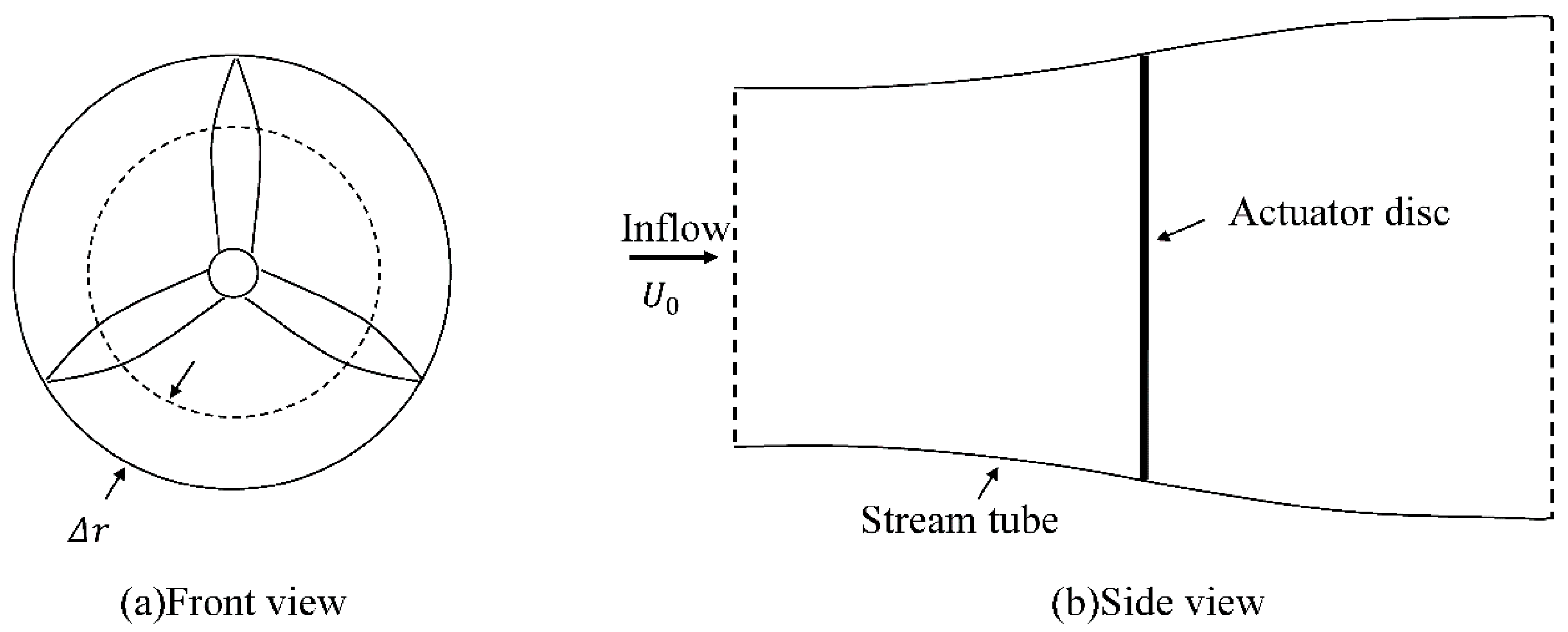The concept of ADM was firstly proposed by Froude [8], following Rankine’s work on the momentum theory of propellers [9]. The fundamental idea of ADM is to use a permeable disc of equivalent area to represent the turbine rotor. The force is evenly distributed on the disc and it is calculated from the velocity of approaching flow and the thrust coefficient of turbine rotor. To account for the rotational feature of rotor, the blade element momentum method (BEM) proposed by Glauert was introduced to the ADM to become the ADM-R [10]. The BEM models the turbine blade as several independent blade elements characterized by their aerodynamic parameters such as drag and lift coefficients. By calculating the force on each blade element, the rotational features of the turbine rotor is considered and the distribution of force on the disc is obtained. ADM/AMD-R has been widely adopted by industry due to its simplicity and relative high accuracy. ALM and ASM modify the ADM/ADM-R by modeling the rotor with actuator line or surface. The performance of ALM and ASM has been studied in references [11,12,13,14].

A widely adopted model to simulate turbulent flow is the Reynolds-averaged Navier–Stokes (RANS) method. The first attempt to simulate turbine wake by RANS adopted the parabolic and axial-symmetric form of the Navier–Stokes equations, which gave a fast calculation. However, it cannot predict the (pressure driven) expansion of the wake properly [15]. Crespo et al. proposed an asymmetric parabolic model, UPWAKE, based on standard k-ε model with specific model constants [16,17]. Cabezón et al. used the standard k-ε model coupled with ADM to evaluate the performance in simulating the turbine wakes [18]. Simulation results showed that the standard k-ε model over-estimated the recovery of turbine wakes due to the under-estimation of turbulence dissipation rates near the turbine. Further investigations showed that the standard k-ε and k-ω models tend to yield diffusive wakes, resulting in over-recovery of the wake velocity but without a distinct peak of turbulence intensity that appeared in wind tunnel experiments [18,19,20,21,22,23]. Réthoré explained the failures of these standard models with the limitations of the Boussinesq hypothesis [19]. Kasmi and Masson then proposed an extended k-ε model, in which a turbulence dissipation zone was added artificially creating a non-equilibrium turbulence in the certain area to address the weakness of the Boussinesq hypothesis [21]. The corresponding results featured lower discrepancy than those from the standard model. Similar approaches were carried out by Cabezón et al. and Rados et al. with acceptable results compared to experiment measurements [18,23]. Réthoré revised Kasmi’s model by importing turbulence production terms and gave a wake prediction with relative higher accuracy [19]. Van der Laan pointed out that in the wake region, where the velocity gradient is high, the constant to parameterize the eddy viscosity should be flow depend. Following this idea he proposed an improved k-ε model which yielded relatively good results in different cases [24,25].

Though various kinds of modified k-ε models had been proposed, many of them were based on the application of non-equilibrium turbulence and the results are heavily dependent on the empirical correction of turbulence dissipation or production. Meanwhile, though many of these k-ε-based models consider the non-equilibrium of turbulence, usually they assume the isotropy of the Reynolds stresses. However, this condition cannot be found in practice, especially in the region near the wind turbine where the turbulent shear is extremely large. Gómez et al. indicated that turbulence anisotropy exists in the turbine wake and this effect is more intense when it is closer to the border of the wake [26]. Reynolds Stress Model (RSM), considering an equilibrium but anisotropic Reynolds stresses, is a potentially good model to simulate the wind turbine wake. Cabezón compared various k-ε-based models and RSM concluding that RSM can give a relatively good simulation of wake deficit in both near and far wake regions and acceptable wake turbulence intensity results [27]. Makridis and Chick simulated the wind turbine wakes with terrain effect using RSM and gave acceptable predictions [28]. Cabezón et al. applied RSM in OpenFOAM simulating the turbine wakes of a large wind farm and concluded that RSM gave a better solution than isotropic model and could be further developed [29].

In the present work, the RSM turbulence model is applied to simulate the wake flow of a single wind turbine mounted on flat terrain. ADM-R is introduced to model the turbine rotor induced forces. Turbine nacelle induced forces is calculated by the drag coefficient of the nacelle. A standard k-ε model and an extended k-ε model are also adopted as contrasts to evaluate the performance of RSM. Finally, the wind flow quantities simulated by three different turbulence models are presented and compared with data from wind tunnel experiments. The relative importance of the RSM is discussed with reference to the performance of predicting the wake flow of turbine machines, and further application in the wind farm sitting, planning and optimization.

2. Governing Equations

Reynolds-averaged Navier–Stokes equations (RANS) are used as the governing equations of the atmospheric boundary layer flowing through wind turbines. Specifically, the governing equations of a stationary incompressible Newtonian fluid can be written in Einstein notation as:

$$\frac{\partial u_i}{\partial x_i}=0$$

(1)

$$\rho {\overline{u}}_j\frac{\partial {\overline{u}}_i}{\partial x_j}=-\frac{\partial p}{\partial x_i}+\frac{\partial }{\partial x_j}\left[\mu \left(\frac{\partial {\overline{u}}_i}{\partial x_j}+\frac{\partial {\overline{u}}_j}{\partial x_i}\right)-\rho \overline{u_i^{\prime }{u}_j^{\prime }}\right]+\rho f_{turb}$$

(2)

where ρ is the density, μ is dynamic viscosity, $-\rho \overline{u_i^{\prime }{u}_j^{\prime }}$ is the Reynolds stress and f_turb is the turbine induced force modeled in Section 5.

3. Reynolds Stress Model

Due to the isotropic Reynolds stresses assumption, the standard k-ε model is not capable of simulating the anisotropy of the turbulent flow [30,31,32]. Abandoning the isotropic Reynolds stresses assumption, the Reynolds-stress model solved the governing equations above together with the transport equations of Reynolds stresses and an equation for the dissipation rate. It yields better prediction in the streamline curvature, swirl, rotation, and rapid changes in strain rate than the k-ε model.

The steady incompressible transport equation for the Reynolds stresses is formulated as:

$$\rho \frac{\partial }{\partial x_k}\left(u_k\overline{u_i^{\prime }{u}_j^{\prime }}\right)=-D_{T,ij}+D_{L,ij}+P_{ij}+{\varphi }_{ij}-{\epsilon }_{ij}$$

(3)

where

• Turbulent diffusion $D_{T,ij}=\frac{\partial }{\partial x_k}[\rho \overline{u_i^{\prime }{u}_j^{\prime }{u}_k^{\prime }}+\overline{p^{\prime }(u_i^{\prime }{\delta }_{kj}+u_j^{\prime }{\delta }_{ik})}],$ modeled as $D_{T,ij}=\frac{\partial }{\partial x_k}\left(\frac{u_t}{\partial x_k}\frac{\partial \overline{u_i^{\prime }{u}_j^{\prime }}}{\partial x_k}\right)$.
• Molecular diffusion $D_{L,ij}=\frac{\partial }{\partial x_k}\left[\mu \frac{\partial }{\partial x_k}(\overline{u_i^{\prime }{u}_j^{\prime })}\right]$.
• Stress production $P_{ij}=-\rho \left(\frac{\partial u_j}{\partial x_k}\overline{u_i^{\prime }{u}_k^{\prime }}+\frac{\partial u_i}{\partial x_k}\overline{u_j^{\prime }{u}_k^{\prime }}\right)$.

Pressure-strain ${\varphi }_{ij}=p^{\prime }\overline{\left(\frac{\partial u_j^{\prime }}{\partial x_i}+\frac{\partial u_i^{\prime }}{\partial x_j}\right)}$ and it is modeled using a linear pressure-strain model [33,34,35,36] as: ${\varphi }_{ij}={\varphi }_{ij,1}+{\varphi }_{ij,2}+{\varphi }_{ij,w}$. The slow pressure-strain term ${\varphi }_{ij,1}=-C_1\frac{\rho \epsilon }{k}\left[\overline{u_i^{\prime }{u}_j^{\prime }}-\frac{2}{3}{\delta }_{ij}\rho k\right]$, $C_1=1.8$; the rapid pressure-strain term ${\varphi }_{ij,2}=-C_2\left[P_{ij}-C_{ij}-\frac{1}{3}{\delta }_{ij}\left(P_{kk}-C_{kk}\right)\right]$, $C_2=0.6$; the wall reflection term ${\varphi }_{ij,w}=C_1^{\prime }\frac{\epsilon }{k}\left(\overline{u_k^{\prime }{u}_m^{\prime }}{n}_k{n}_m{\delta }_{ij}-\frac{3}{2}\overline{u_i^{\prime }{u}_k^{\prime }}{n}_j{n}_k-\frac{3}{2}\overline{u_j^{\prime }{u}_k^{\prime }}{n}_i{n}_k\right)\frac{C_l{k}^{3/2}}{\epsilon d}+C_2^{\prime }\left({\varphi }_{km,2}{n}_k{n}_m{\delta }_{ij}-\frac{3}{2}{\varphi }_{ik,2}{n}_j{n}_k-\frac{3}{2}{\varphi }_{jk,2}{n}_i{n}_k\right)\frac{C_l{k}^{3/2}}{\epsilon d}$, $C_1^{\prime }=0.5$, $C_2^{\prime }=0.3$, $n_k$ is the $x_k$ component of the unit normal to the wall, $d$ is the normal distance to the wall and $C_l={C_{\mu }}^{3/4}/\kappa$ where $\kappa =0.4187$ is the Von Kármán constant.

Dissipation ${\epsilon }_{ij}=2v\overline{\frac{\partial u_i^{\prime }}{\partial x_k}\frac{\partial u_j^{\prime }}{\partial x_k}}$ and it is modeled as ${\epsilon }_{ij}=\frac{2}{3}{\delta }_{ij}\rho \epsilon$.

The turbulent viscosity is modeled as ${\mu }_t=\rho C_{\mu }\frac{k^2}{\epsilon }$, turbulent kinetic energy is computed as: $k=\frac{1}{2}\overline{u_i^{\prime }{u}_i^{\prime }}$ and the scalar dissipation rate ε is computed from the following equations: $\rho \frac{\partial }{\partial x_j}\left(\epsilon u_i\right)=\frac{\partial }{\partial x_j}\left[\left(\mu +\frac{u_t}{{\sigma }_{\epsilon }}\right)\frac{\partial \epsilon }{\partial x_j}\right]C_{\epsilon 2}\frac{\epsilon P_{ii}}{2k}-C_{\epsilon 2}\frac{\rho {\epsilon }^2}{k}$ with C_μ = 0.09, σ_k = 1, σ_ε = 0.82, C_ε1 = 1.44, C_ε2 = 1.92, C₁ = 1.8, C₂ = 0.6.

4. Standard k-ε Model and Extended k-ε Model

To evaluate the performance of the RSM, the standard k-ε model and an extended k-ε model are also studied for comparison. The standard k-ε model and the extended k-ε model are briefly introduced below. The standard k-ε model solves the Navier-Stokes equations by introducing the transport equations for the turbulence kinetic energy k and dissipation rate ε as [35]:

$$\rho \frac{\partial }{\partial x_i}\left(k{u}_i\right)=\frac{\partial }{\partial x_j}\left[\left(\mu +\frac{{\mu }_t}{{\sigma }_k}\right)\frac{\partial k}{\partial x_j}\right]+P_k-\rho \epsilon +S_k$$

(4)

$$\rho \frac{\partial }{\partial x_i}\left(\epsilon u_i\right)=\frac{\partial }{\partial x_j}\left[\left(\mu +\frac{{\mu }_t}{{\sigma }_{\epsilon }}\right)\frac{\partial \epsilon }{\partial x_j}\right]+C_{1\epsilon }{P}_k\frac{\epsilon }{k}-C_{2\epsilon }\rho \frac{{\epsilon }^2}{k}+S_{\epsilon }$$

(5)

where: $P_k={\mu }_t\left(\frac{\partial u_i}{\partial x_j}+\frac{\partial u_j}{\partial x_i}\right)\frac{\partial u_i}{\partial x_j}$ is the production of kinetic energy.

S_k is the source term for the turbulence kinetic energy and S_k = 0 for both the standard k-ε model and extended k-ε model in the present study. S_ε is the source term for turbulence dissipation. In present study, S_ε = 0 for the standard k-ε model and $S_{\epsilon }={\wp }_{\epsilon }$ for the extended k-ε model described below. C_1ε = 1.44 and C_2ε = 1.92 are constants and σ_k = 1.0 and σ_ε = 1.3 are the Prandtl numbers for k and ε.

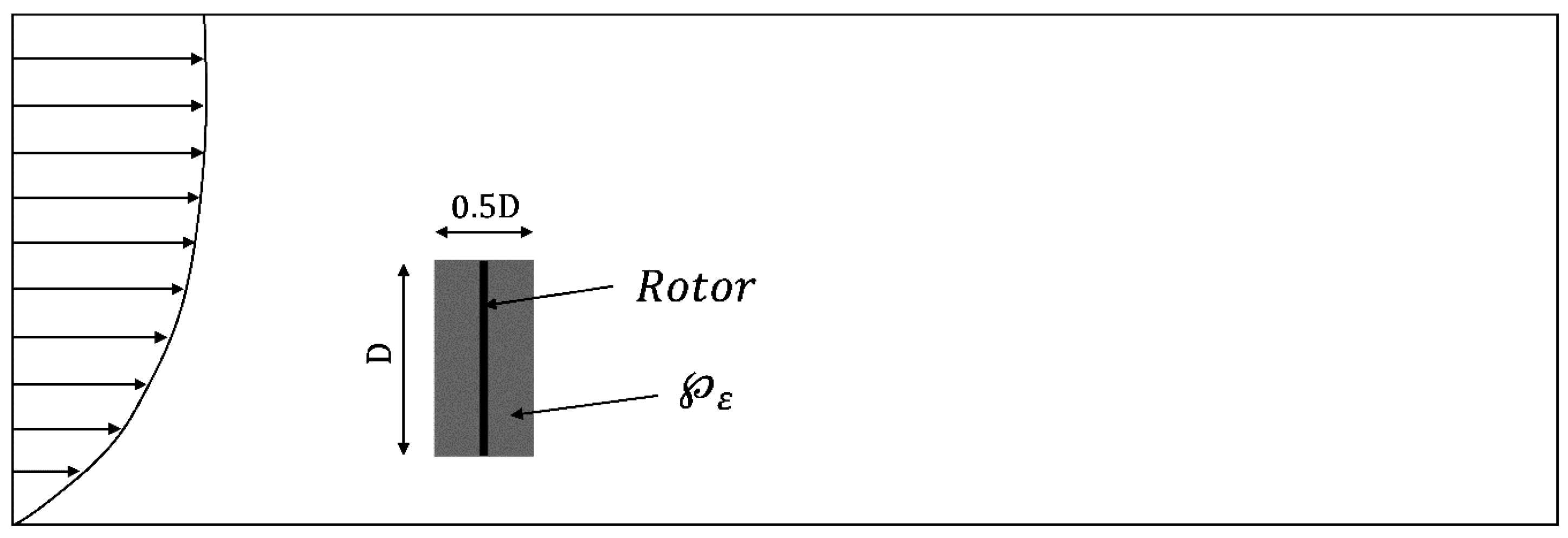
The extended kε model improves the performance in predicting the turbine wakes by introducing artificial turbulence dissipation. As shown in Figure 1, an extra turbulence dissipation ${\wp }_{\epsilon }$ is added to the volume upstream and downstream within approximately 0.25 D of the turbine.

The artificial turbulence dissipation ${\wp }_{\epsilon }$ is defined as:

$${\wp }_{\epsilon }=C_{\epsilon 4}\frac{P_k^2}{\rho k}$$

(6)

where C_ε4 is a parameterized constant set to be 0.37. For more specific details readers are referred to Kasmi and Masson [21].

5. Turbine Modelling

The computation of the governing equations requires knowledge and modeling on the turbine induced forces f_turb. In this study, the turbine induced forces consists of two parts: the rotor induced forces f_rotor and the nacelle induced forces f_nac.

The rotor induced forces f_rotor is modeled by ADM-R purposed by Mikkelsen [12]. This approach models the real wind turbine rotor with a permeable disc of equivalent area and with the blade-induced forces applied, as shown in Figure 2.

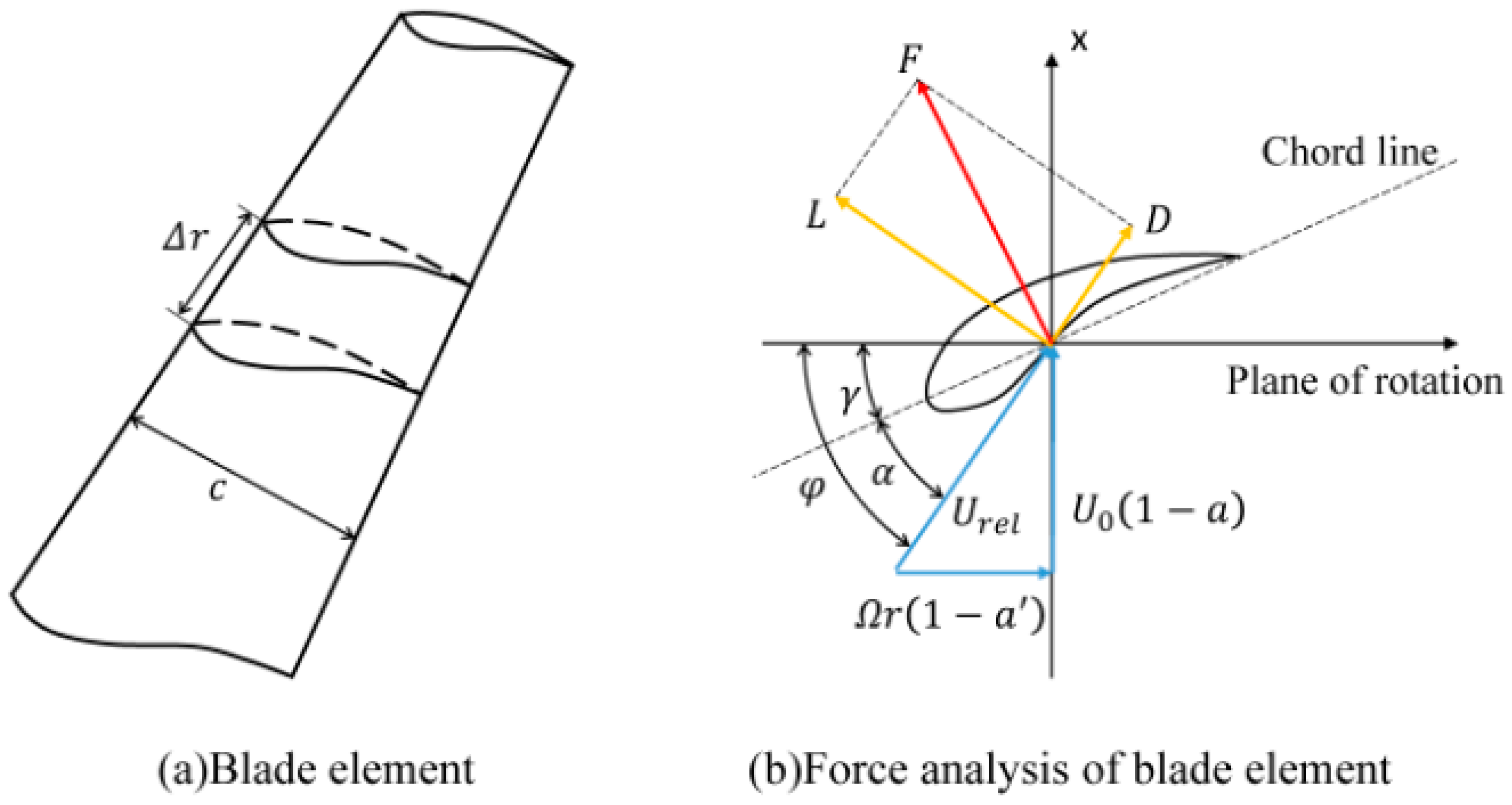
The distribution of forces on the disc are calculated by the Blade Element Momentum theory (BEM) [37]. The blade is divided into N elements. The induced forces on each blade element include the drag forces and lift forces:

$$(L,D)=\frac{1}{2}\rho U_{rel}^{2}c\Delta r\left(C_L{e}_L,C_D{e}_D\right)$$

(7)

$$F=\frac{1}{2}\rho U_{rel}^{2}c\Delta r\left(C_L{e}_L+C_D{e}_D\right)$$

(8)

where C_L and C_D are the lift coefficient and drag coefficient respectively extracted from tabulated airfoil data, e_L and e_D are unit direction vectors, Δr is the radial length of blade elements and c is the chord length. $U_{rel}=\left({\mathbf{U}}_0\left(1-a\right), {\mathsf{\Omega }}_r\left(1-a^{\prime }\right)\right)$ is the relative velocity of incident flow. It composed of the relative axial velocity $U_0\left(1-a\right)$ and relative tangential velocity ${\mathsf{\Omega }}_r\left(1-a^{\prime }\right)$ of the incident flow relative to the blade element. $U_0$ is the velocity of the stream-wise approaching flow, $\mathsf{\Omega }$ is the angular velocity of the wind turbine, r is the distance from the hub to the points representing the blade elements. a and a’ are the axial and tangential introduction factors, respectively. The angle of attack is defined as:

$$\alpha =\phi -\gamma$$

(9)

where $\phi ={\tan }^{-1}\left[\frac{U_0\left(1-a\right)}{{\mathsf{\Omega }}_r\left(1-a^{\prime }\right)}\right]$ and γ is the pitch angle of the blade element shown in Figure 3.

By applying the BEM, the axial and tangential introduction factors a and a’ could be calculated and the relative velocity of the incident flow U_rel can also be obtained. Considering the annular area the blade element sweeps through in one rotation is ΔA = 2πrΔr and the number of blades is B, the forces on each annular disc area can be calculated as:

$$F^{\prime }=\frac{B\cdot F}{\Delta A}=\frac{1}{2}\frac{\rho U_{rel}^{2}Bc}{2\pi r}\left(C_L{e}_L+C_D{e}_D\right)$$

(10)

The body forces acting on the actuator disc are functions of the disc thickness Δz:

$$f_{rotor}^{\prime }=\frac{F^{\prime }}{\Delta z}$$

(11)

In order to avoid singular behavior and numerical instability, body forces are gradually applied on the actuator disc by taking convolution of the local body forces $f_{rotor}^{\prime }$ and the regularisation kernel $n_{\delta }$:

$$f_{rotor}=f_{rotor}^{\prime }\ast {\eta }_{\delta }$$

(12)

where

$${\eta }_{\delta }=\frac{1}{{\delta }^3{\pi }^{3/2}}\exp \left[-{\left(p/\delta \right)}^2\right]$$

(13)

and δ is a constant that serves to adjust the concentration of the regularized load. It is taken equal to the value of a grid side length in this study, p is the distance between the grids points and the points representing the blade elements.

Meanwhile, nacelle was modeled by porous media and the nacelle induced force is described as:

$$f_{nac}=\frac{F_{nac}}{A_{nac}\Delta z}=-\frac{1}{2}\frac{\rho u_0^2{C}_{\mathrm{D},nac}}{\Delta z}{e}_x$$

(14)

where $A_{nac}$ is the front area of nacelle, $u_0$ is the velocity at center of rotor, $e_x$ is unit vector in the stream direction and $C_{\mathrm{D},nac}$ = 1.0 is the drag coefficient of the nacelle which has a range of 0.8–1.2 [21,38].

6. Numerical Experiment

6.1. Computation Domain and Turbine Specifications

To validate the RSM, simulation results will be compared with wind tunnel measurements carried out by Chamorro and Porté-Agel in the St. Anthony Falls Laboratory atmospheric boundary-layer wind tunnel [39]. The experiment studied a miniature turbine consisting of a three-blade GWS/EP-6030 × 3 rotor and a small DC generator motor with rotor diameter of 0.15 m and hub height of 0.125 m. The ratio of distance between ground and the bottom of the rotor to the rotor radius is 0.67 which is of the same order as for real turbines of large capacity (≥2 MW). The cylindrical nacelle is of 0.015 m diameter and 0.03 m length. The effect of the tower is neglected in the study. The computational domain is 4.32 m in stream-wise (L_x), 0.72 m in span-wise (L_y) and 0.46 m in height (L_z) as shown in Figure 4. The wind turbine is placed at the center of the wind tunnel in span-wise and six rotor diameters (0.9 m) behind the inlet in stream-wise.

The radial variation of the chord length and pitch angle are obtained from Wu and Porté-Agel [40]. The blade is modeled with a flat plate. The experimental results on the lift and drag coefficients on the plate for different angle of attack are adopted [41].

The turbine rotated with an angular velocity of 1120 rpm with a tip speed ratio ≈ 4 and an inflow velocity of 2.2 m/s and turbulence intensity of 0.08 at the hub height. The tip speed ratio has been modified to match that of the full-scale turbines, which is usually between 3 and 8 [42]. Other tip speed ratio, within the range of 3 and 10, was also adopted in many wind-tunnel based studies of wind-turbine wakes for single turbines as well as different configurations in wind farms [4]. The thrust coefficient is 0.53 based on the calculation of axial force. The Reynolds number of the experiment is about 4000. Though there is discrepancy between the experiment and the reality, it is capable of the basic characteristics of the turbine wake [43]. All numerical settings are corresponding to the experiment described by Chamorro and Porté-Agel [39] and Wu and Porté-Agel [40].

6.2. Boundary Conditions

The inflow has a logarithmic mean velocity profile and a turbulence intensity profile corresponding to the experiment. The profile of turbulence dissipation rate is also given as $\epsilon =C_{\mu }^{3/4}\frac{k^{3/2}}{l}$ where k is the kinetic energy, C_μ = 0.09 and the turbulent length l = 0.15 m is equal to one rotor diameter.

The bottom layer has a no-slip wall boundary condition with 0.03 mm roughness height and 0.5 roughness constant. The Reynolds stress at the cells adjacent to wall are approximated in terms of the kinetic energy as $\frac{\overline{u^{\prime }{u}^{\prime }}}{k}=1.098$, $\frac{\overline{v^{\prime }{v}^{\prime }}}{k}=0.655$, $\frac{\overline{w^{\prime }{w}^{\prime }}}{k}=0.247$ and $-\frac{\overline{u^{\prime }{w}^{\prime }}}{k}=0.255$. Near wall regions are approximated by a standard wall function [36] and the wall reflection is considered by adopting the wall reflection term φ_ij,w in the pressure-strain as mentioned in Section 3. Reynolds stress model. The outlet has a zero diffusion flux for all flow variables and an overall mass balance correction. All the other boundaries are set to be zero-shear slip walls.

6.3. Solution Methods and Grid Sensitivity

The Semi-Implicit Method Pressure Linked Equation (SIMPLE) algorithm is adopted as the pressure-velocity coupling method to solve the Navier-Stokes equations. The momentum is discretized using a second order upwind scheme. The turbulence kinetic energy, turbulent dissipation rate and the Reynolds stresses are then discretized using a first order upwind scheme. All the calculation is implemented by the Fluent software in the ANSYS 14.5 package. An Intel Xeon E5-2630 CPU with 12 cores and 2.60 GHz is used. The RAM is 64 GB. Eight nodes are used in the Fluent for the parallel computation.

The computational domain was uniformly divided by Nx × Ny × Nz grid points. The actuator disc used to model the turbine rotor was covered by Ry × Ry grid points. To test the grid sensitivity of the RSM model, three different mesh schemes were applied as shown in

Table 1. Mesh schemes.

Case	Nx	Ny	Nz	Lx(m)	Ly(m)	Lz(m)	Elements	Ry	Rz
Coarse	106	29	19	4.32	0.72	0.46	52,920	7	7
Normal	136	43	27	4.32	0.72	0.46	147,420	10	10
Fine	186	67	43	4.32	0.72	0.46	512,820	15	15

. For the densest grid, it takes around 45 s for the calculation using standard k-ε model and extended k-ε model and around 90 s using RSM.

7. Results and Discussion

The RSM is compared with the standard k-ε, extended k-ε model and the wind tunnel data from Chamorro and Porté-Agel [39] and Wu and Porté-Agel [40] in simulating the turbine wakes velocity and turbulence intensity. Kinetic shear stress $-\overline{u^{\prime }{w}^{\prime }}$ is calculated by RSM and plotted against measurements data to prove its accuracy. Then, the affected area, distribution, variation and recover tendency of turbine wakes are investigated using the RSM. Finally, the grid sensitivity of RSM is discussed.

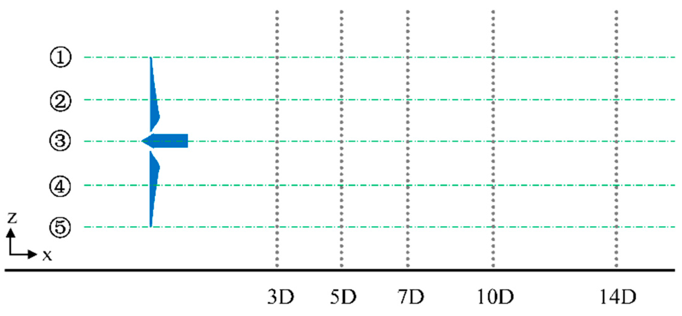
Due to intense velocity reduction and turbulence increase, two turbines are seldom found within a distance of 3 D in most modern wind farms [4]. Therefore, the effects in the area beyond 3 D will be considered. Specifically, they are cross-sections at 3 D, 5 D, 7 D, 10 D and 14 D downstream. More detailed studies at −0.7 D, −0.6 D …0.6 D, 0.7 D relative to a cross-section downstream at 5 D of the turbine are also conducted.

7.1. Vertical Distribution of Stream-Wise Velocity

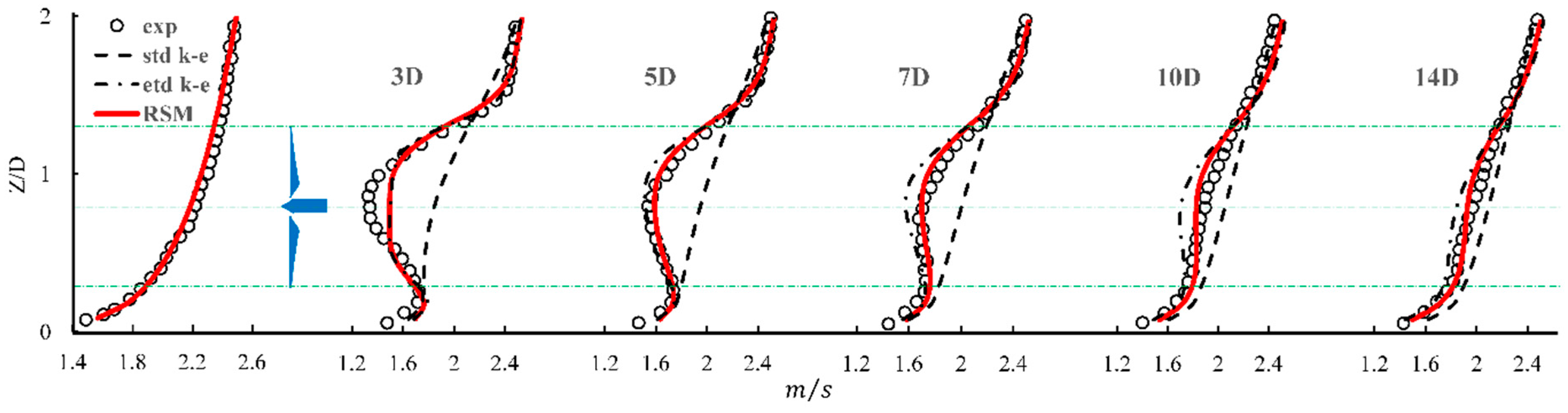
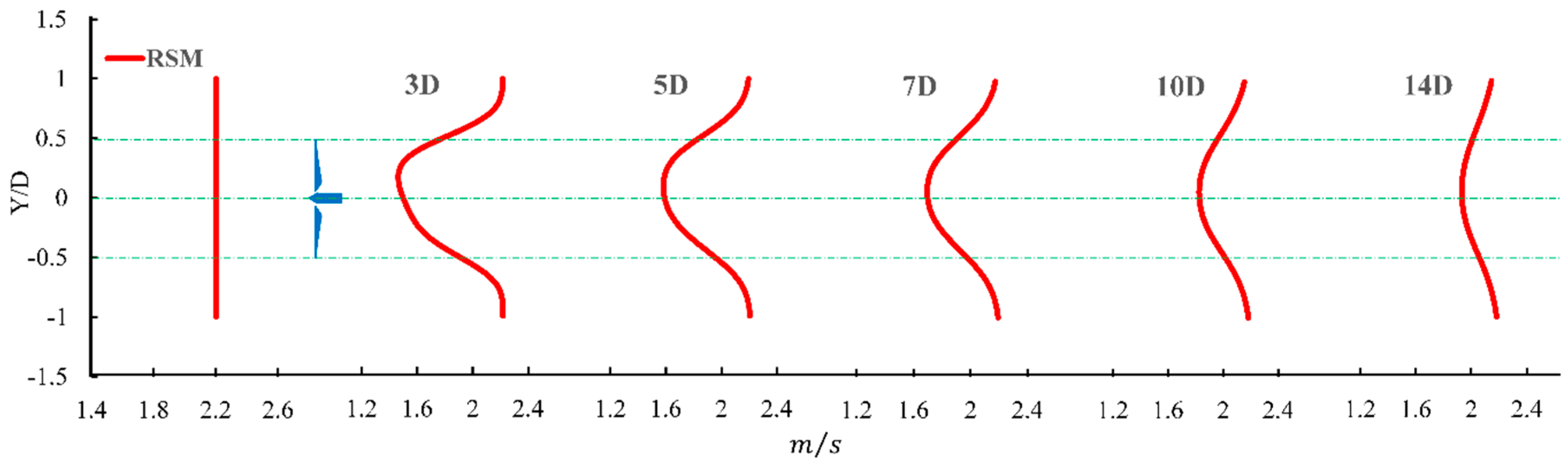
Figure 5 shows the vertical distribution of stream-wise velocity of the approaching flow and turbine wakes. It indicates a loss of velocity appearing right after the air flowing over the turbine, and the maximum loss occurs at the hub height. The RSM presents good prediction of the wakes velocity, and there is just slight difference between the simulation results and measurements data.

The extended k-ε model showed acceptable performance, but not as good as the RSM. The recovery of velocity was insufficient due to the artificial turbulence dissipation added in the extended k-ε model. The standard k-ε model, as expected, failed to simulate velocity of turbine wakes, especially in the area within 10 D. The characteristics of the diffusive wake of over-estimating the recovery of wake velocity are presented as mentioned in the introduction. Two parameters—5 points averaged relative error (δ_5p) and maximum relative error (δ_max) are defined to quantify the performance of different simulations. ${\delta }_{5p}={{\displaystyle \sum }}_{i=1}^5\left(|V_i^{EXP}-V_i^{SIM}|/V_i^{EXP}\right)/5$ is the average of relative error at the height of: ① top of the rotor, ② middle of upper half rotor, ③ hub, ④ middle of lower half rotor and ⑤ bottom of the rotor (see Figure 6), which are typical heights to define a wake profile. ${\delta }_{max}=\left(|V^{EXP}-V^{SIM}|/V^{EXP}\right)$ is the maximum relative error within the height from ① the top of the rotor to ⑤ bottom of the rotor (see Figure 6). V^EXP is the value from wind tunnel experiments and V^SIM is the value from the CFD simulation.

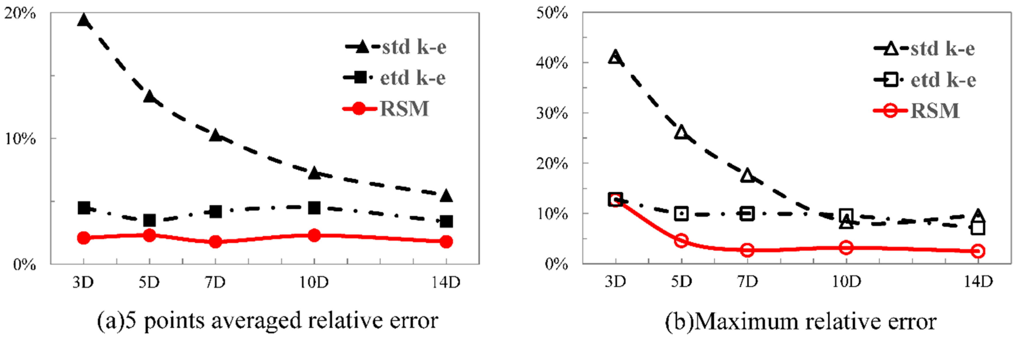
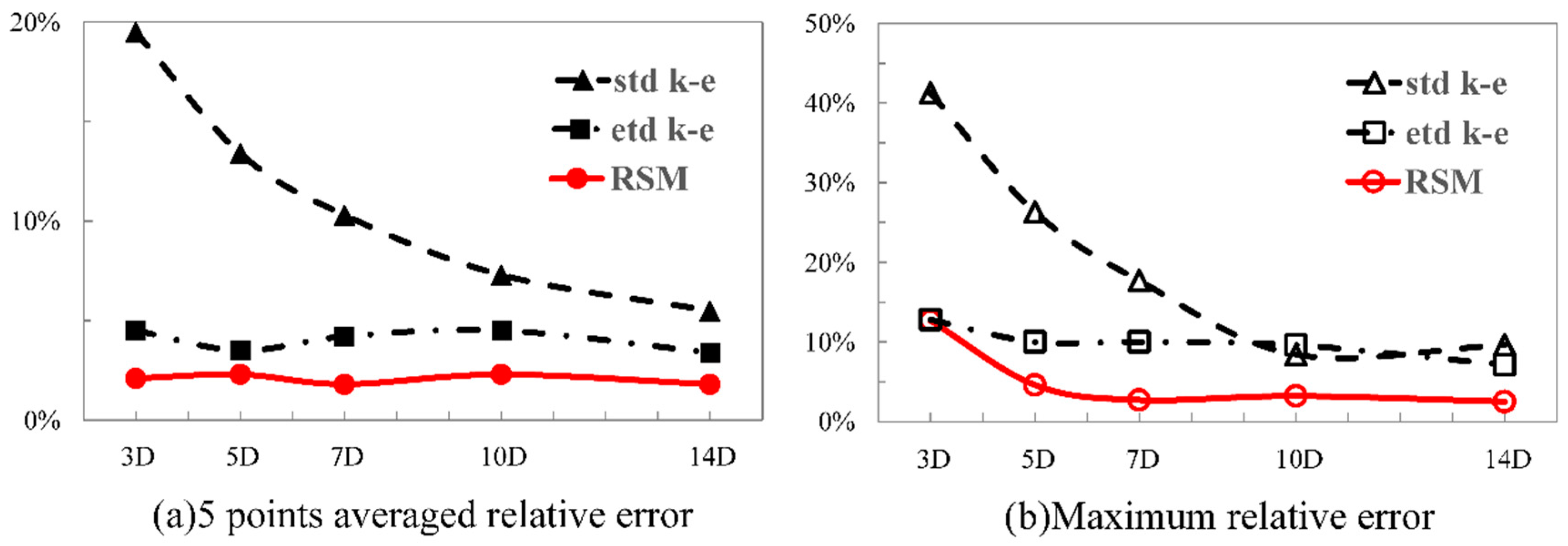
Figure 7 shows the five points averaged relative error and maximum relative error on the velocity simulated by standard k-ε , extended k-ε model and the RSM. Same remarks as for Figure 5 could be made, i.e., the standard k-ε model fails to predict the turbine wake velocity with ${\delta }_{5p}^{k-\epsilon }$ ranging from 5% to 20% and ${\delta }_{\max }^{k-\epsilon }$ between 8% and 41%. On the other hand, the extended k-ε model reduces ${\delta }_{5p}^{Kasmi}$ to around 5% and ${\delta }_{\max }^{Kasmi}$ to 10%–15%. Finally, the RSM performs well to predict the wake velocity with ${\delta }_{5p}^{RSM}$ around 2% and ${\delta }_{\max }^{RSM}$ under 10%. The latter is only 4% of 5 D downstream.

7.2. Lateral Distribution of Stream-Wise Velocity

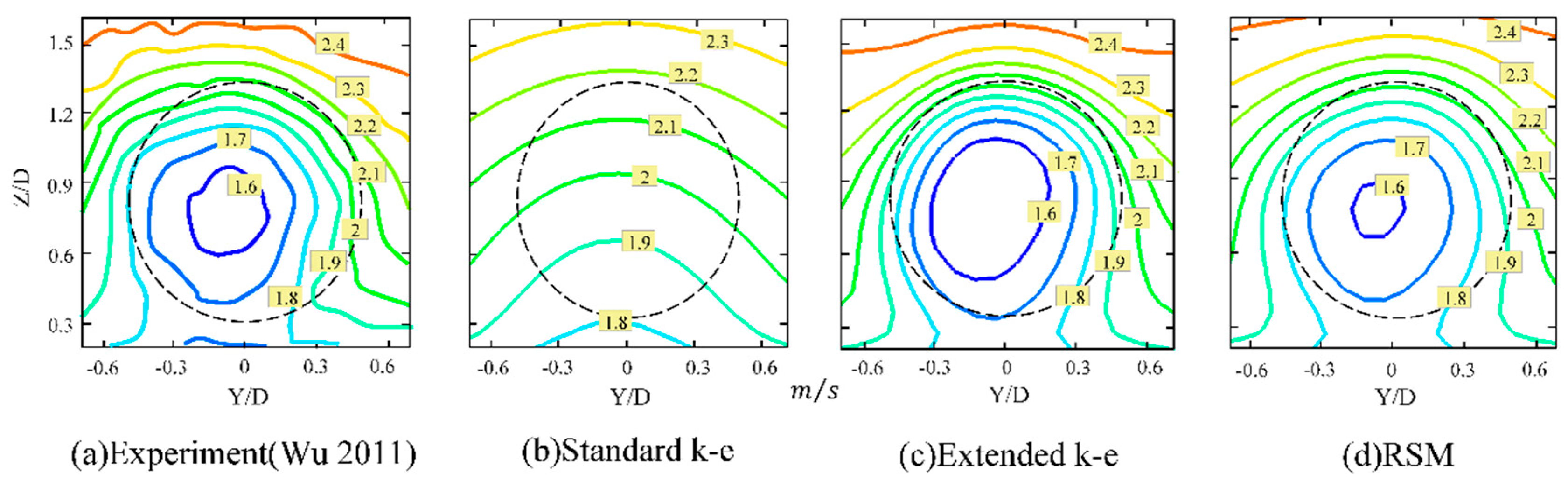
Figure 8 shows the contours of stream-wise velocity at 5 D downstream. The position ranges from −0.7 D–0.7 D (0.0 corresponds to axial centerline of the turbine) horizontally and 0.2 D–1.6 D (0.0 is at the ground) vertically and the dash line represent border of rotor rotation. From the result of wind tunnel measurements, we can see that wakes velocity distributes asymmetrically in both vertical and horizontal directions. The vertical asymmetry results in logarithmic mean velocity profile of the approaching flow and the horizontal asymmetry results in swirl of the turbine wake. Clearly, standard k-ε model failed to simulate the swirl of wake. On the other hand, both the extended k-ε model and the RSM capture the swirl of flow. The extended k-ε model slightly under-estimates the velocity of turbine wake at 5 D while the RSM performs well.

The horizontal distribution of wake velocity is also of interest, especially in the transition zone and its total area. Figure 9 shows the horizontal profiles of stream-wise velocity of the approaching flow and turbine wakes at hub height. With a lack of experimental data, only the RSM simulation results are presented. The velocity of air is greatly reduced due to the wake effect. The maximum reduction occurs at the center of the wakes and it decreases in radial direction away from the central plane. The profile of wakes velocity approaches a Gaussian distribution. Meanwhile, the area with velocity reduction is expanding with the stream-wise distance, but limited within ± D in the across-wind direction (0.0 is the hub position). The asymmetry of wakes is seen again, but it is not significant after 5 D.

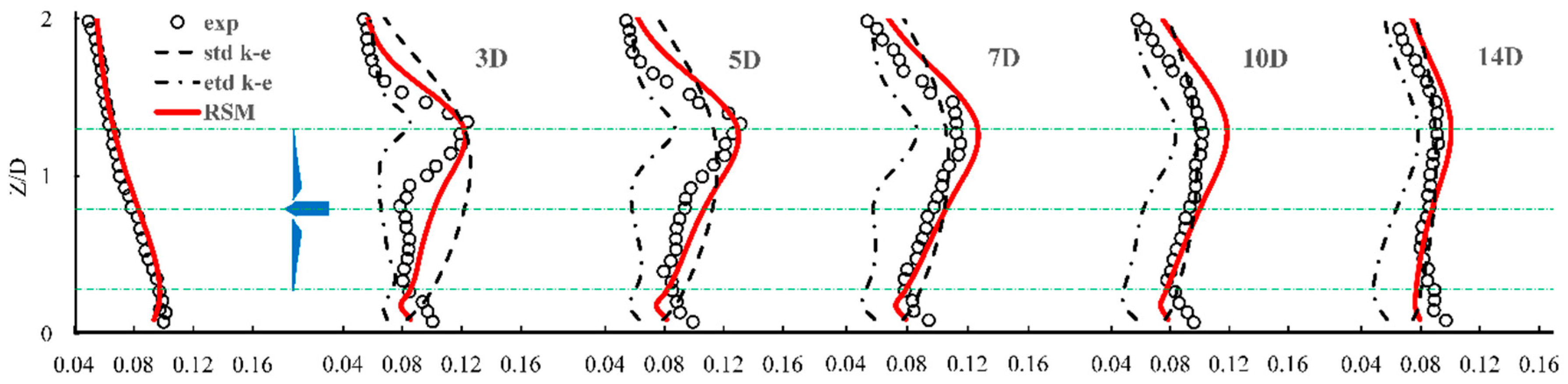
7.3. Vertical Distribution of Stream-Wise Turbulence Intensity

Figure 10 shows the vertical distribution of stream-wise turbulence intensity (TI) of the approaching flow and turbine wakes. TI takes up different definition in different models: In wind tunnel measurements, TI is defined as ${\sigma }_u/{\overline{u}}_{hub}$. In RSM, TI is defined as $\sqrt{\overline{u^{\prime }{u}^{\prime }}}/{\overline{u}}_{hub}$. In the standard k-ε model and the extended k-ε model, TI is approximated by the kinetic energy using the assumption of isotropic turbulence as (k/1.5)^1/2/${\overline{u}}_{hub}$. In the present study, wind tunnel measurements show that the highest TI appears at the top of rotor tips and it decreases with down-stream distance. The standard k-ε model can capture the peak location of the TI, in general. However, it fails to predict the distribution and over-estimates the whole TI profile. The feature of the diffusive wake shown indicates the failure to simulate the distinct peak of TI. The extended k-ε model can predict the trend of TI declining and shows distinct peak of TI. But it under-estimates the TI due to the artificial turbulence dissipation zone added. The RSM shows acceptable performance in predicting the highest level of TI and the smooth profile of TI, and the simulation results are clearly better than those from the standard k-ε model and the extended k-ε model. It should be noted that all three kinds of model underestimate the TI close to ground. This is because both the k-ε model and the RSM approximate the kinetic stresses at ground by using the kinetic energy whereas the actual boundary condition of the kinetic stresses are unknown.

The 5 points averaged relative error and maximum relative error are plotted as Figure 11. Though the prediction in the wake velocity is good, yet the extended k-ε model fails to simulate the turbine wake turbulence velocity with error ${\delta }_{5p}^{Kasmi}$ bigger than 20% and error ${\delta }_{\max }^{Kasmi}$ up to 41%. On the contrary, the standard k-ε model fails to predict the wind turbine wake velocity accurately, but it shows an acceptable performance in predicting the TI, especially at locations beyond 7 D with error ${\delta }_{5p}^{k-\epsilon }$ varies from 4% to 28% and less than 10% beyond 7 D. However, the error ${\delta }_{\max }^{k-\epsilon }$ ${\delta }_{\max }^{k-\epsilon }$ is 57% because the TI at 3 D downstream is extremely over-estimated. Finally, the RSM shows good ability to simulate the profile of TI with error ${\delta }_{5p}^{RSM}$ around 10% and error ${\delta }_{\max }^{RSM}$ around 20%.

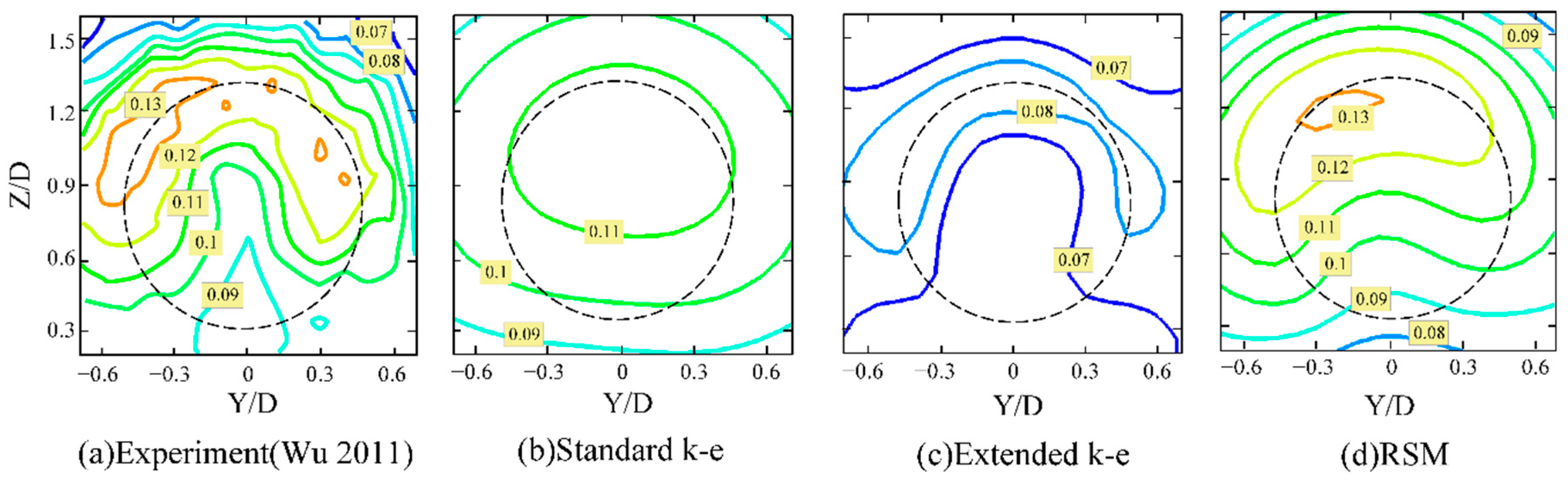
7.4. Lateral Distribution of Stream-Wise Turbulence Intensity

Figure 12 shows the contours of TI at 5 D downstream. The biggest TI from experiment appears at the upper half border of the rotor. Due to the interaction between the blade tip and air that produces vortices, the TI at this area has a sudden jump. Also due to the non-uniformity of the approaching flow, the fluctuating wind speed at great height is higher than that at lower height when wind blows over the turbine resulting in the non-asymmetry of TI in the vertical direction. Similar to the velocity, the TI is also horizontally non-asymmetric distributed. Simulation results show that the standard k-ε model fails to capture this feature with incorrect TI estimates. The extended k-ε model can basically capture this feature of the TI distribution, but it grossly under-estimates the TI. Simulation results of RSM shows good agreement with wind tunnel results, i.e., both vertical and horizontal non-asymmetry in the velocity and TI are observed, the TI amplification due to the tip-air interaction and good estimates in the values.

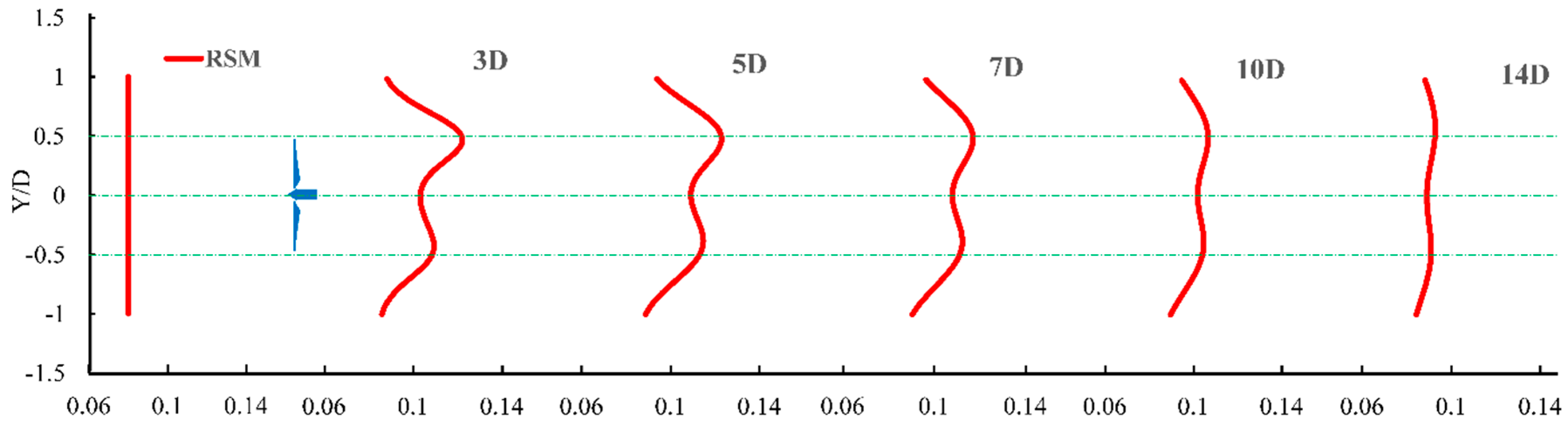
Similarly, the horizontal profiles of stream-wise turbulence intensity of the approaching flow and turbine wakes at hub height is presented as Figure 13. Again, due to the lack of experiments data, only the RSM simulation results are presented. Results show that the turbulence intensity is bimodal distributed with two peaks at R and −R, accounting for the tip-air interaction. The two peak values are different due to the air rotation. The asymmetry is noted less significant after 5 D.

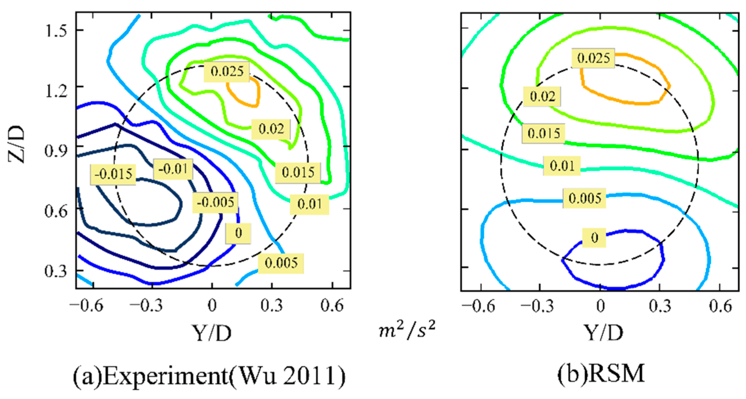
7.5. Spatial Distribution of the Kinetic Stresses

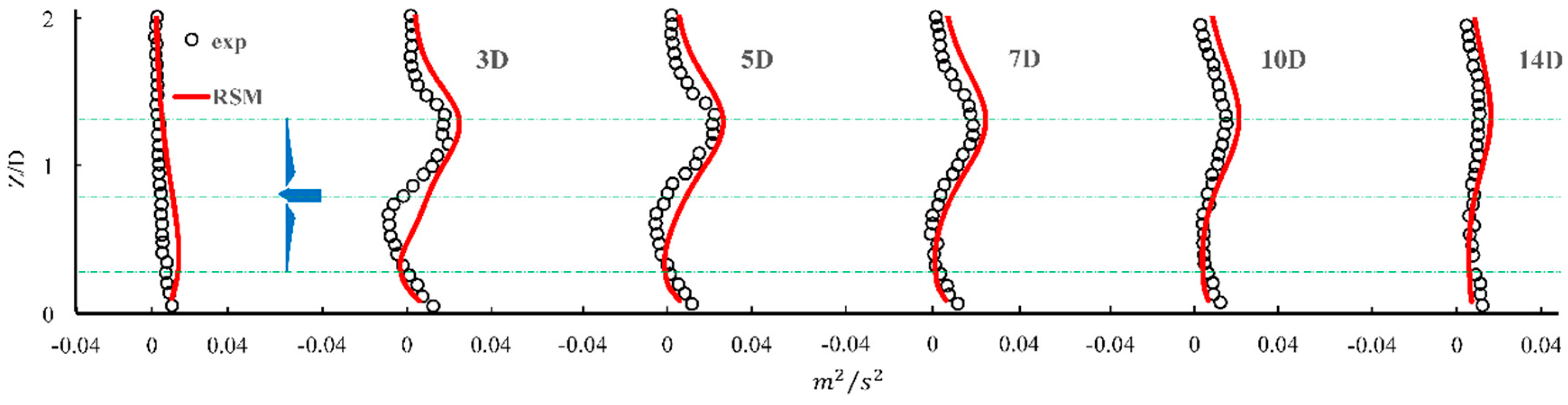
The vertical distribution of kinetic shear stress $-\overline{u^{\prime }{w}^{\prime }}$ of the approaching flow and turbine wakes are shown as Figure 14. RSM is the only model amongst the three ones studied that assumes an anisotropic turbulence stress. Therefore, only the RSM results are compared with the wind tunnel data. Similar to the turbulence intensity, a strong shear occurs at the top of rotor tip, and a large negative shear is noted at the bottom of the rotor tip. This is because the tip of blade has the largest velocity relative to air resulting in the strongest shear between the blade and air. The RSM simulates this phenomenon well, and the magnitudes of simulation results are slightly higher than that from the wind tunnel experiments. The difference decreases further downstream. Figure 15 shows the contour of kinetic shear stress $-\overline{u^{\prime }{w}^{\prime }}$ at 5 D. The experimental data shows a tilted distribution of the turbulence stress. This asymmetry, once again, is due to rotation of air. The RSM results give a similar distribution but to a less tilted extend. This is because the ADM is unable to simulate accurately the tip vortex which can maintain the rotation of the wake. By simulating the kinetic shear stress $-\overline{u^{\prime }{w}^{\prime }}$ of the wake, the RSM features a good ability to predict the turbulence kinetic stress with consideration of anisotropy of the turbine wakes.

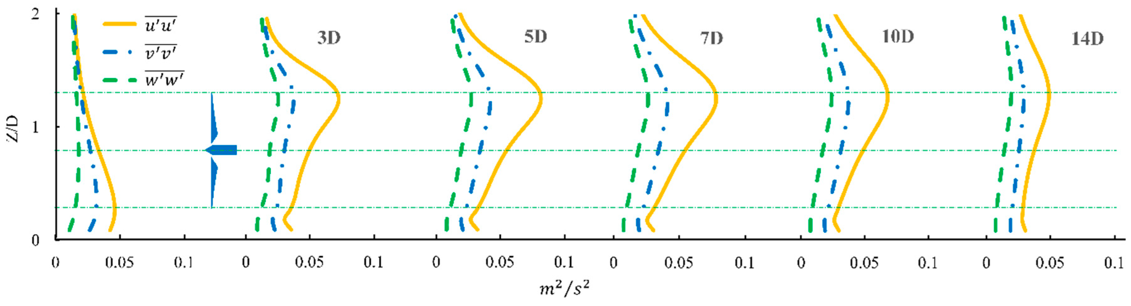
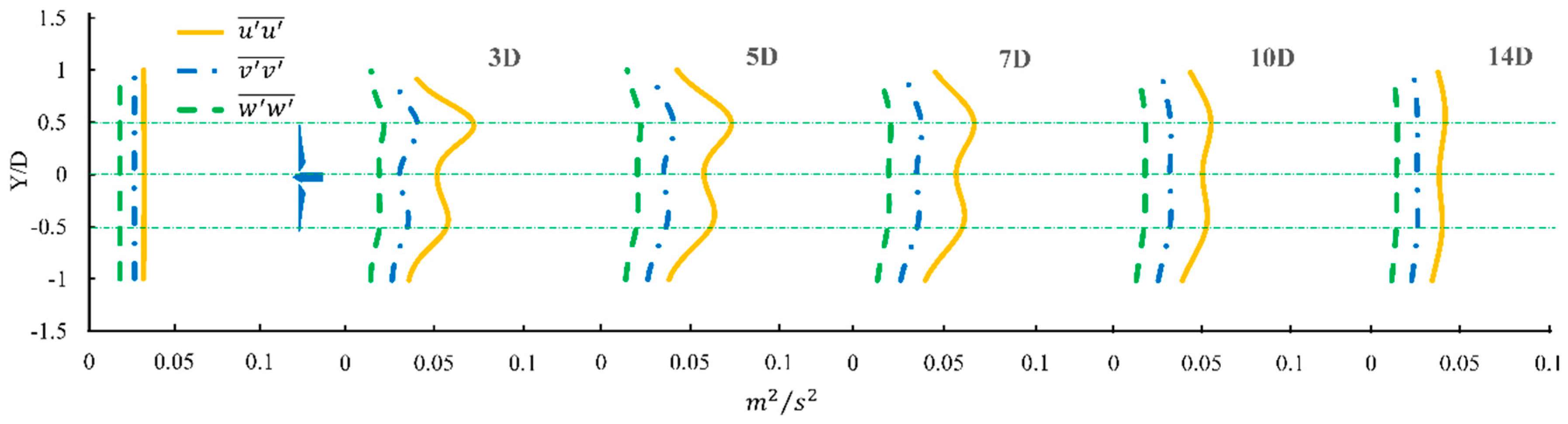
To evaluate the anisotropy of the turbine wakes, the kinetic stresses $\overline{u^{\prime }{u}^{\prime }}$, $\overline{v^{\prime }{v}^{\prime }}$ and $\overline{w^{\prime }{w}^{\prime }}$ are simulated by the RSM. Figure 16 and Figure 17 show the vertical and horizontal distribution of these three kinetic stresses. It is noted that the approaching flow (1 D ahead of turbine) has been assumed isotropic, except close to ground where the friction will cause some anisotropy.

When air flows over the turbine, a strong anisotropy is shown at the tip area. Stress $\overline{u^{\prime }{u}^{\prime }}$ is dramatically amplified by the tip-air interaction and is much larger than stress $\overline{v^{\prime }{v}^{\prime }}$ and $\overline{w^{\prime }{w}^{\prime }}$ with $\overline{u^{\prime }{u}^{\prime }}>\overline{v^{\prime }{v}^{\prime }}>\overline{w^{\prime }{w}^{\prime }}.$ This anisotropic feature of turbine wake accounts for the under-estimation of the turbulence intensity by the extended k-ε model where isotropy of Reynolds stresses is assumed.

7.6. Recovery of the Turbine Wake

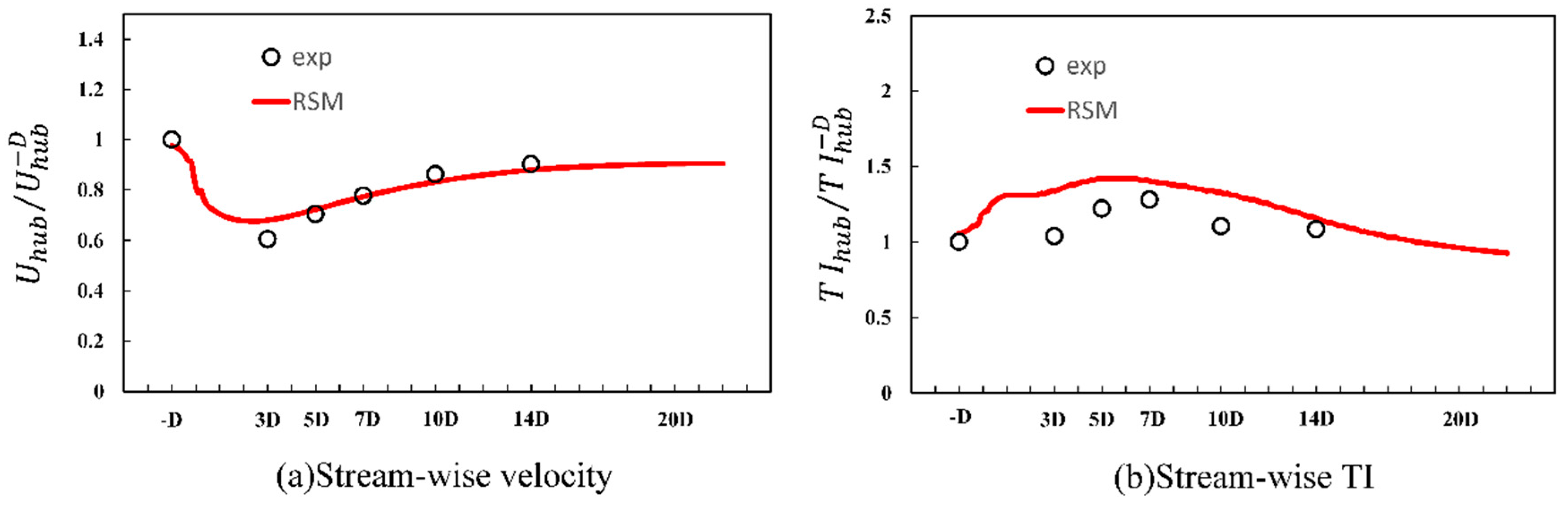
Figure 18 shows the stream-wise velocity and turbulence intensity at hub height. The wake velocity drops quickly immediately after the air flows over the turbine and it picks up the velocity gradually. The recovery of wakes velocity can reach 90% at around 10 D and at the final 91% at around 16 D. The wakes turbulence intensity increases gradually with downstream distance and reaches the maximum at around 5 D. The recovery of wake turbulence intensity slowed down after 15 D and then reached the same level with approaching flow.

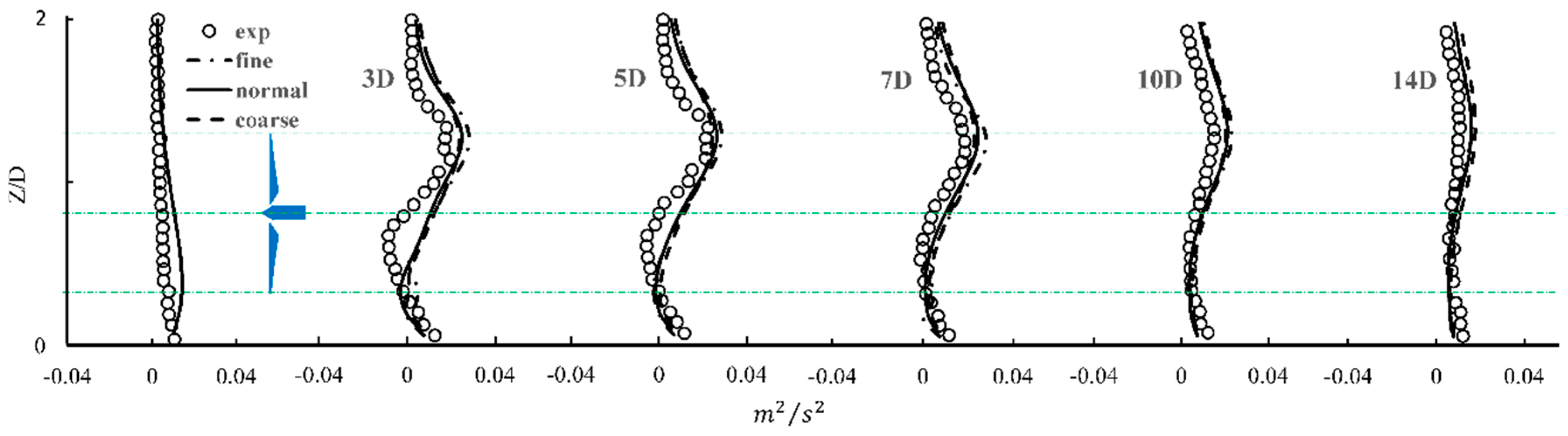
7.7. Grid Sensitivity of RSM Model

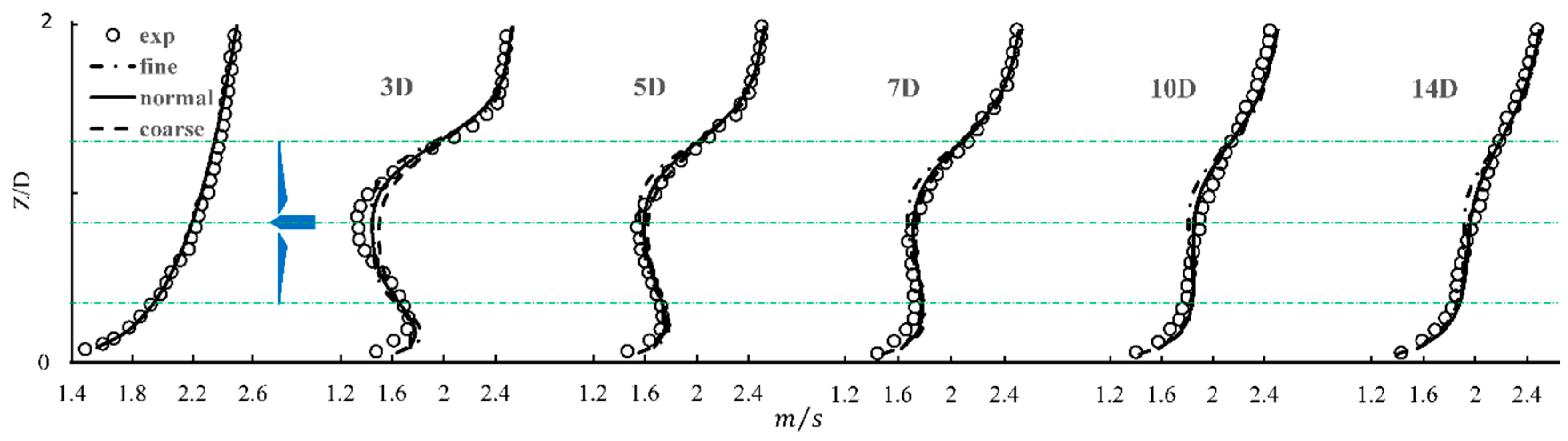
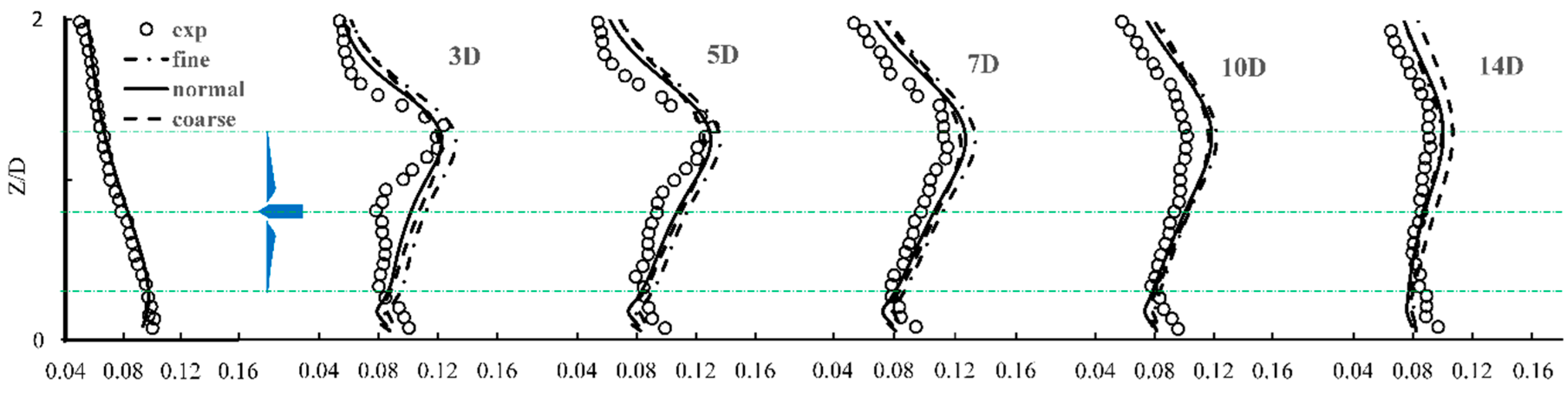
To test the grid sensitivity of RSM model, three different mesh schemes are prepared as Table 2. Simulation results of the turbine wakes velocity, turbulence intensity and kinetic shear stress $-\overline{u^{\prime }{w}^{\prime }}$ are presented as Figure 19, Figure 20 and Figure 21. The RSM showed low sensitivity to the grid resolution. Three kinds of mesh schemes yield similar results in the wakes velocity and kinetic shear stress $-\overline{u^{\prime }{w}^{\prime }}$. Only less than 10% difference is noted when using a coarse grid scheme to predict the turbulence intensity.

A “normal” dense grid resolution (actuator disc is covered by 10 × 10 grid points) is considered sufficient to model the turbine wakes velocity, turbulence intensity and turbulence stress for engineering purpose. When simulating a wind farm with several turbines with other complicated conditions, the amount of calculation will increase quickly. A “coarse” dense grid resolution (actuator disc is covered by 7 × 7 grid points) may yield acceptable results with less computation effort.

8. Conclusions

The standard k-ε model has been used to simulate ABL flowing through wind turbines in recent years for many different cases. Most of them yield inaccurate predictions in either the turbine wakes velocity or turbulence intensity. Based on The standard k-ε model, many modified k-ε models are proposed to improve the simulation results. Many of them adopted non-equilibrium turbulence in the model and resulted in better prediction of wake velocity. But the simulation on the wake turbulence intensity is still inaccurate on the near wakes or far wakes. Because most of these modified k-ε models are still based on the isotropic Reynolds stresses assumption. But existing researches had also noted the anisotropic turbine wakes. To account for this feature, Reynolds Stress Model (RSM), coupled with actuator disc model with rotation (ADM-R) are used in this study to simulate the wake velocity, turbulence intensity and kinetic shear stress of a miniature wind turbine. The simulation results are compared with wind tunnel test data, and simulation results from the standard k-ε model and a well noted extended k-ε model.

Simulation results showed that the RSM is capable to accurately predict the turbine wakes velocity, turbulence intensity and kinetic stress in presented circumstance. The asymmetric features of the miniature wind turbine wakes due to non-uniform inflow and wake rotation are also captured by RSM. In contrast, the standard k-ε model fails to predict wakes velocity and it over-estimates the turbulence intensity before 10 D. Moreover, it fails to simulate the rotation of wakes. The extended k-ε model has good prediction on the wakes velocity, but it under-estimates the wakes turbulence intensity as expected due to the isotropy of Reynolds stresses.

Both the RSM simulation results and experimental data show that the wind velocity decreases after air flowing over the miniature turbine and the maximum reduction occurs at hub height while the turbulence intensity is greatly amplified at the blade tip. The recovery of wake velocity will attain 90% at around 10 D downstream and achieves a steady 91% at around 16 D. The wake turbulence intensity increases gradually and reaches a maximum at around 5 D. The recovery of wake turbulence intensity slows down after 15 D and eventually the turbulence intensity merges in with that as the approaching flow. Further investigation by RSM shows that the horizontal profile of wakes velocity can be approximated with a Gaussian distribution, and that for the turbulence intensity can be approximated with a bimodal distribution. The horizontal asymmetry of wake is minimal after 5 D and the influence of wakes effect is limited within ± D in the across-wind direction. The anisotropy of turbine wakes is also affecting the distribution of the kinetic stresses $\overline{u^{\prime }{u}^{\prime }}$, $\overline{v^{\prime }{v}^{\prime }}$ and $\overline{w^{\prime }{w}^{\prime }}$ in the RSM. Results show that the wake of the miniature turbine is clearly anisotropic, especially at the blade tip. Stress $\overline{u^{\prime }{u}^{\prime }}$, and was obviously larger than $\overline{v^{\prime }{v}^{\prime }}$ and $\overline{w^{\prime }{w}^{\prime }}$, accounting for the under-estimation of turbulence intensity with the extended k-ε model.

Finally, the RSM shows low sensitivity to grid resolution—an actuator disc covered by 10 × 10 grid points is considered sufficient to simulate turbine wakes velocity, turbulence intensity and kinetic stresses, and an actuator disc covered by 7 × 7 grid points can also yield similar results. In addition, for the densest grid, it takes around 45 s for the calculation using standard k-ε model and extended k-ε model and around 90 s suing RSM. Though RSM takes twice the computational effort as k-ε models, the actual difference is really small and is totally acceptable.