Spatial and Temporal Traffic Variation in Core Networks: Impact on Energy Saving and Devices Lifetime ^†

Abstract

We assess the impact of traffic variations on energy consumption and devices lifetime in a core network. Specifically, we first define a model to control the spatial as well as the temporal variations of traffic. We generate different sets of traffic matrices by adopting our model, which are then used as input to an energy-aware algorithm, with the aim of finding the set of Line Cards (LCs) in Sleep Mode (SM) for each traffic matrix. Given this output, we are able to compute different evaluation metrics, including: the total energy consumption, the normalized lifetime as a consequence of activation/deactivation of network devices, and the total network profitability (i.e., the monetary gain/loss for the operator). Our results show that the temporal variation of traffic affects the LCs energy consumption, but has a limited impact on their lifetime. Moreover, the spatial variation of traffic is no obstacle for energy saving. Eventually, the frequency of the power cycles, introduced by the energy-aware algorithm, is particularly important for the lifetime of LCs. Finally, we show that positive total profitability is achieved in most of the considered cases.

1. Introduction

Energy consumption of core networks is constantly increasing due to constantly increasing traffic demands and despite the improving energy-efficiency in terms of power required to provide certain capacity (Watt/bps). One of the most promising approaches to reduce energy consumption of Internet Protocol (IP)-over-Wavelength Division Multiplexing (WDM) networks is the application of Sleep Mode (SM) to network devices (see, e.g., the surveys [1,2]). The main idea of this approach is to dynamically deactivate network resources when they are unused and activate them again when needed. However, the application of SM has an impact on the devices lifetime (i.e., the time between one failure and the following one) [3]. Specifically, the authors have shown in [3] that the lifetime of network devices is heavily influenced by HardWare (HW) parameters of the devices as well as by the strategy used to put devices into SM or Active Mode (AM). Therefore, a core network experiences energy and lifetime variations as a consequence of the activation/deactivation of its resources.

The choice whether a subset of devices shall be put into SM is highly dependent on the evolution of traffic over time. More precisely, networks are dimensioned to satisfy peak traffic demands. However, traffic varies both in time and space. At night few users generate traffic, resulting in a low utilization of network devices. Moreover, if the network spans across different time zones, the periods of low utilization will not occur at the same time in all regions of the network, but will be shifted across the time zones.

In this context, several questions arise, like: How to model temporal and spatial traffic variations in a core network? What is the influence of both temporal and spatial traffic variations on the energy savings and on the devices lifetime? How does the difference across time zones affect the results? The goal of this paper is to provide answers to such questions. More in depth, we first propose a simple traffic model that captures temporal and spatial traffic variation. We then focus on a network scenario adopting a realistic network topology, as well as the traffic variations derived from our model. Moreover, a sophisticated Mixed-Integer Linear Programming (MILP) model with realistic parameters is used to design the network, i.e., choose which devices to install and how to configure them. The designed network is then taken as input for dynamic operation over time, i.e., selection which devices to put into SM as a consequence of the traffic variation while ensuring Quality of Service (QoS) constraints. Specifically, we exploit a heuristic approach to dynamically find the set of active LCs versus time. Finally, we compute the achieved energy savings as well as the effect on devices lifetime and profitability, showing the influence of the proposed traffic model on these evaluation metrics.

Previous works in the literature mainly investigated the impact of temporal variations of traffic on the energy savings (see particularly [4,5]). In the work [6] we went two steps further by: (i) considering the devices lifetime; and (ii) considering the impact of spatial traffic distribution on both lifetime and energy savings. We extend [6] by (i) explicitly considering the impact of temporal traffic variation on lifetime and energy savings; (ii) performing a sensitivity analysis of lifetime variation as a consequence of different combinations of input HW parameters; and (iii) estimating the total profitability of the network as the difference between electricity savings and reparation costs triggered by lifetime variation. In addition, the presented MILP formulation used to design the input topology enforces single-shortest-path routing of IP traffic demands over the IP topology in the reference network, which is an aspect in general not considered by any related work in energy-efficient multilayer core networks. We believe that the presented results can provide fruitful indications on how future networks should be operated in order to be energy-efficient and lifetime-aware.

The rest of the paper is organized as follows. Section 2 presents related work regarding traffic modeling in the context of green backbone networking. Our traffic model, covering both temporal and spatial variations, is detailed in Section 3. Section 4 describes the network model. The evaluation scenario is detailed in Section 5. Results are analyzed in Section 6, and conclusions are drawn in Section 7. Details of the network design MILP formulation as well as tables of notation for parameters and variables can be found in the Appendix A.

2. Related Work

Traffic modeling has been an important research topic for many years due to the changing nature of traffic (e.g., driven by newer and newer applications and various Internet access methods). In general, traffic is an important input in different research areas and in different types of networks. While temporal and spatial traffic distributions are widely covered for wireless networks (e.g., [7,8]), this issue has been relatively unexplored for wired networks (particularly in the context of green core networking). This is first due to the fact that node mobility does not affect the amount and distribution of traffic exchanged among the nodes in core networks. In addition, while mobile networks often take into account variation of traffic in terms of packets, such analysis is challenging in the context of core networks, due to the extremely high amount of installed capacities in the devices.

Focusing on traffic modeling, an analytical model covering spatio-temporal bursty traffic is proposed in [9] for communications networks in multicluster systems. Differently from [9], we focus on traffic demands between all node pairs in the network described by a set of traffic matrices covering a certain period of time.

Focusing on variations of traffic over time, sinusoidal functions are usually used as a parametrized model [4,5,10,11,12,13,14,15,16,17,18,19,20,21,22]. Traffic variation in the context of saving energy is the focus only of [4,5]. The authors propose a model of aggregated traffic taking the set of considered time periods (by default spanning 24 h) as well as maximum and minimum traffic volumes as parameters. Our model extends them with (sub)sets of time periods when traffic is high, low, increasing, and decreasing. To the best of our knowledge, no related work exists that provides a traffic model including parameters to change spatial traffic distribution over time in a controlled way. Some works consider a shift of traffic according to the time zone in which nodes generating traffic are located (see [23,24,25,26,27,28,29]). No variation of spatial traffic distribution is studied in these articles, though. We refer to Table VIII of [2] for a detailed overview of traffic data used in the works on green core networking.

Summarizing, the contribution of this work w.r.t. previous works is the following: (i) a traffic model covering both temporal and spatial traffic variations; (ii) a sophisticated MILP formulation to design a realistic reference network (with single-shortest-path IP routing) used as input for the dynamic network operation; (iii) evaluation of the impact of controlled temporal and spatial traffic variations on both the energy consumed by LCs and their lifetime; (iv) assessment of the profitability as a difference between total electricity savings and total reparation costs in the network.

3. Traffic Model

We propose a simple traffic model to control both the temporal and spatial variations of traffic over time. Notation used in the traffic model is summarized in

Table A2. Notation of parameters used for traffic model, network design (MILP), network operation (EWA), and evaluation.

	Symbol	Description
General and MILP	$G=(V,E)$	undirected physical supply network with set of nodes V and set of physical supply links $E\subseteq \left\{\left\{i,j\right\}\subseteq V^2:i\ne j\right\}$
	$H=(V,L)$	undirected logical supply network with set of nodes V and set of logical supply links $L\subseteq \left\{\left\{i,j\right\}\subseteq V^2:i\ne j\right\}$
	C	capacity of a lightpath
	B	number of wavelengths per fiber
	P	set of all (undirected) paths through G on which capacity modules can be installed
	$P_i$	set of all paths from P where one of the end nodes is $i\in V$
	$P_{i,j}$	set of all paths from P whose end nodes are the end nodes of $\left(i,j\right)\in L$
	$P_e$	set of all paths from P that traverse physical supply link $e\in E$
	N	set of routers that can be installed in the network
	$R_n$	capacity of router $n\in N$
	δ	maximum lightpath utilization, $\delta \in (0,1]$
	${\kappa }^{\mathrm{oxc}}$	CapEx cost of installing an OXC
	${\kappa }_n^{\mathrm{ipr}}$	CapEx cost of installing router $n\in N$
	${\kappa }^{\mathrm{lp}}$	CapEx cost of installing a lightpath with LC
	${\kappa }_e^{\mathrm{f}}$	CapEx cost of installing a fiber on physical supply link $e\in E$
EWA	$W_L$	threshold on the utilization of the last lightpath on a logical link to trigger attempts to release lightpaths, $W_L\in [0,1)$
	$W_H$	threshold on the utilization of the last lightpath on a logical link to trigger attempts to establish new lightpaths, $W_H\in (0,1]$
	ψ	maximum utilization of the last lightpath on a logical link, $\psi \in (0,1]$
	$X_i^{LC}$	number of LCs installed at node $i\in V$
Time and traffic	T	set of considered time periods in the proposed traffic model
	$\widehat{T}$	set of time periods covered by traffic measurements
	$T_{low}$	set of time periods with low traffic, $T_{low}\subseteq T$
	$T_{high}$	set of time periods with high traffic, $T_{high}\subseteq T$
	$T_{inc}$	set of time periods with increasing traffic, $T_{inc}\subseteq T$
	$T_{dec}$	set of time periods with decreasing traffic, $T_{dec}\subseteq T$
	$\Delta t$	length of each time period $t\in T$
	$\widehat{\Delta }t$	length of each time period $t\in \widehat{T}$
	$A_{max}^{a,b}$	maximum traffic demand value for the node pair $\left(a,b\right)\in V^2$ in the proposed traffic model
	$A_{min}^{a,b}$	minimum traffic demand value for the node pair $\left(a,b\right)\in V^2$ in the proposed traffic model
	${\tilde{d}}_{a,b}(t)$, $d_{a,b}(t)$	traffic demand between the ordered node pair $a,b\in V^2$ during time period $t\in T$ without (with) spatial variation (Equations (5) and (1))
	$d_{a,b}$	maximum traffic demand between the ordered node pair $a,b\in V^2$ (Equation (8))
	$d_i^{+}$, $d_i^{-}$	maximum emanating (ending) traffic demand at node $i\in V$ (Equation (A11))
	${\widehat{d}}_{a,b}(t)$	measured traffic demand between the ordered node pair $a,b\in V^2$ during time period $t\in \widehat{T}$
	s	scaling factor to account for increased traffic demands with respect to the time when the original traffic data ${\widehat{d}}_{a,b}(t)$ was captured
	Θ	TZM with ${\theta }_{a,b}$ denoting an element of the TZM Θ, $\left(a,b\right)\in V^2$
	Γ	SVM with ${\gamma }_{a,b}$ denoting an element of the SVM Γ, $\left(a,b\right)\in V^2$
	k	time displacement parameter, $k\in \{1,\cdots ,|T|-1\}$
	${\zeta }_{a,b}$	number of time periods by which the demand between nodes $\left(a,b\right)\in V^2$ is shifted temporally due to spatial traffic variation
Evaluation	${\pi }^{\mathrm{lp}}$	power of a LCs (W)
	$A{F}^{sleep}$	ratio between the failure rates of an LCs dynamically switched between sleep and active modes and of the LCs kept active
	χ	weight for the frequency of the active-sleep-active mode cycles of a LCs (h/cycle)
	$r_{MTTR}$	Mean Time To Repair (MTTR) of a LCs (h)
	$r_{FR}$	Failure Rate (FR) of a LCs (failure/h)
	$r_{Wh}$	cost of energy (USD/Wh)
	$r_{CM}$	hourly rate of a reparation crew member (USD/h/period)

in the Appendix A.

We consider a network with a set of nodes V, and a set of time periods T for evaluation of power consumption during network operation. The length of each time period $t\in T$ is $\Delta t$. A traffic matrix $D(t)$ at time period $t\in T$ describes traffic demands between all node pairs in the network. It is composed of elements $d_{a,b}(t)$ containing (directed) traffic demands exchanged between each ordered node pair $a,b\in V^2$.

The traffic matrices $D(t)$ for all $t\in T$ are obtained in the following two steps. First, we focus on temporal traffic variation, i.e., all traffic demands follow the same (relative) changes over time, without changes of spatial traffic distribution. In the second step, we add parameters to our model in order to vary spatial traffic distribution over time in a controlled way.

3.1. Temporal Traffic Variation

We start out with the assumption that traffic is periodic (day-night pattern) with the period length equal to $\left|T\right|·\Delta t$, where $\left|T\right|$ denotes cardinality of the set T. We distinguish the subsets of time periods $T_{low}\subseteq T$ and $T_{high}\subseteq T$ corresponding to a set of low-demand time periods and a set of high-demand time periods, respectively. Furthermore, we consider linear traffic increase over a set of time periods $T_{inc}\subseteq T$, and linear traffic decrease over a set of time periods $T_{dec}\subseteq T$ as shown in Figure 1a. The traffic demand ${\tilde{d}}_{a,b}(t)$ between a node pair $\left(a,b\right)\in V^2$ is described as:

$$\begin{array}{c}\hfill {\tilde{d}}_{a,b}(t)=\left\{\begin{array}{cc}{A}_{min}^{a,b}\hfill & \mathrm{if}t\in T_{low},\hfill \\ \frac{A_{max}^{a,b}-A_{min}^{a,b}}{|T_{inc}|}t+A_{min}^{a,b}+\hfill \\ -(A_{max}^{a,b}-A_{min}^{a,b})\frac{|T_{low}|}{|T_{inc}|}\hfill & \mathrm{if}t\in T_{inc},\hfill \\ A_{max}^{a,b}\hfill & \mathrm{if}t\in T_{high},\hfill \\ \frac{A_{min}^{a,b}-A_{max}^{a,b}}{|T_{dec}|}t+A_{max}^{a,b}+\hfill \\ -(A_{min}^{a,b}-A_{max}^{a,b})\frac{|T_{low}|+|T_{inc}|+|T_{high}|}{|T_{dec}|}\hfill & \mathrm{if}t\in T_{dec}.\hfill \end{array}\right.\end{array}$$

(1)

The model with its parameters allows not only for the investigation of the influence of traffic amplitude $(A_{max}^{a,b}-A_{min}^{a,b})$ on network energy consumption, but also the influence of the pace of traffic increase $(A_{max}^{a,b}-A_{min}^{a,b})/\left|T_{inc}\right|$ and decrease $(A_{min}^{a,b}-A_{max}^{a,b})/\left|T_{dec}\right|$ on network energy consumption.

The traffic demand curve ${\tilde{d}}_{a,b}(t)$ is different for each node pair $\left(a,b\right)\in V^2$ due to the values $A_{max}^{a,b}$ and $A_{min}^{a,b}$ (see the secondary y-axis of Figure 1a). However, we assume in this step that the relative demand ${\tilde{d}}_{a,b}(t)/A_{max}^{a,b}$ (taking values in the range $\left[0,1\right]$) is the same for all node pairs $\left(a,b\right)\in V^2$ (shown in the primary y-axis of Figure 1a). Temporal traffic variation does not change spatial traffic distribution over time if the ratio $A_{min}^{a,b}/A_{max}^{a,b}$ is equal for all traffic demands ${\tilde{d}}_{a,b}(t)$, and if the sets $T_{low}$, $T_{inc}$, $T_{high}$, and $T_{dec}$ are identical for all traffic demands ${\tilde{d}}_{a,b}(t)$. This is usually not the case in realistic networks, therefore we consider also spatial traffic variation over time in the next step.

The length of each time period $t\in T$ is set to $\Delta t=$ 1 h in Figure 1a in order to make it easy to analyze (particularly in the comparison between the discrete data and continuous data). We change the period length to $\Delta t=$ 5 min in Figure 1b, and show (using discrete data) a comparison with the sinusoidal model from [5]. The maximum and minimum demands ($A_{max}^{a,b}$ and $A_{min}^{a,b}$) for both models are assigned with the same values. The increasing and decreasing trends are the same for both models (particularly consider the curve by Lange and Gladisch shifted by a quarter of a day, i.e., $\left|T\right|\Delta t/4$). Durations of $T_{low}$, $T_{high}$, $T_{inc}$, and $T_{dec}$ can be adjusted to make the match between the two models even closer than in Figure 1b.

3.2. Spatial Traffic Variation

In order to be able to control the spatial traffic variation over time, we focus on the sets of time periods $T_{low}$, $T_{inc}$, $T_{high}$, and $T_{dec}$. More precisely, we consider their circular shifting (as explained below), leaving the ratio $A_{min}^{a,b}/A_{max}^{a,b}$ fixed for all $\left(a,b\right)\in V^2$. Wide-range realistic backbone networks often spread over more than one time zone. To account for the temporal shift in traffic due to effects arising from this, we introduce a Time Zone Matrix (TZM)

$$\mathrm{\Theta }=\left(\begin{array}{ccc}{\theta }_{0,0}& \cdots & {\theta }_{0,\left|V\right|-1}\\ ⋮& \ddots & ⋮\\ {\theta }_{\left|V\right|-1,0}& \cdots & {\theta }_{\left|V\right|-1,\left|V\right|-1}\end{array}\right).$$

(2)

The value ${\theta }_{a,b}\in \mathbb{Z}$ for $\left(a,b\right)\in V^2$ determines the number of time periods the demand curve for node pair $a,b$ has to be shifted temporally due to the fact that a and b lie in time zones differing from a reference time zone. The matrix $\mathrm{\Theta }=0$ is used for a network located completely within the reference time zone.

In order to introduce controlled changes of spatial traffic distribution, we define a Spatial Variation Matrix (SVM)

$$\mathrm{\Gamma }=\left(\begin{array}{ccc}{\gamma }_{0,0}& \cdots & {\gamma }_{0,\left|V\right|-1}\\ ⋮& \ddots & ⋮\\ {\gamma }_{\left|V\right|-1,0}& \cdots & {\gamma }_{\left|V\right|-1,\left|V\right|-1}\end{array}\right),$$

(3)

similarly to the TZM, but with values ${\gamma }_{a,b}\in [-1,1]$ for $\left(a,b\right)\in V^2$. Additionally, we introduce a time displacement parameter $k\in \{0,\cdots ,|T|-1\}$. Then for $\left(a,b\right)\in V^2$ the value

$${\zeta }_{a,b}=\lfloor k·{\gamma }_{a,b}\rceil ,$$

(4)

defines the number of time periods each demand curve should be shifted temporally due to spatial traffic variation (the function $\lfloor x\rceil$ stands for rounding of x to the nearest integer value). More precisely (and taking into account both ${\theta }_{a,b}$ and ${\zeta }_{a,b}$), the spatially varied traffic demand $d_{a,b}(t)$ for $t\in T$ is computed as

$$d_{a,b}(t)={\tilde{d}}_{a,b}(t-{\theta }_{a,b}-{\zeta }_{a,b}+m·\left|T\right|),$$

(5)

where the period multiplicity $m\in \mathbb{Z}$ is defined as

$$m=⌊\frac{t-{\theta }_{a,b}-{\zeta }_{a,b}}{\left|T\right|}⌋.$$

(6)

Figure 2 shows the effect of the time displacement parameter k on an exemplary 3-node network with demands for three node pairs (with zero TZM) over a day with the time granularity $\Delta t$ set to 1 h for simplicity. Initially, these single demands follow curves as defined in Section 3.1 (discretized), with different values for $A_{max}^{a,b}$ and $A_{min}^{a,b}$ (21, 28, 42 and 3, 4, 6 units, respectively), which results in a total traffic curve of the same type (Figure 2a). For spatial variation, the single demand curves are shifted according to the SVM

$$\mathrm{\Gamma }=\left(\begin{array}{ccc}0& -0.4127& 1\\ 0& 0& -0.1415\\ 0& 0& 0\end{array}\right),$$

(7)

so that for higher values of k the total traffic variation in the network appears as a distorted version of the initial total traffic curve (compare the red solid curve in Figure 2a with the red solid curves in Figure 2b–d). The total demand curve is different for different values of k and the same Γ despite the fact that the total amount of traffic over a day ${\sum }_{t\in T}{\sum }_{\left(a,b\right)\in V^2}{d}_{a,b}(t)$ is equal for all cases.

4. Network Model

We explain the architecture assumptions of the IP-over-WDM network model in the first subsection. The network design method and the network operation method are explained in the following two subsections. Notation of parameters and variables used in this work is summarized in respectively Table A2 and

Table A3. Notation of variables used for network design (MILP), network operation (EWA), and evaluation.

MILP	${\widehat{f}}_{i,j}^{a,b}$	$\in \{0,1\}$—whether or not the traffic demand from node $a\in V$ to $b\in V$ traverses the logical link $\left(i,j\right)\in L$ in the direction from $i\in V$ to $j\in V$
	${\widehat{\phi }}_{i,j}$	$\in \{0,1\}$—whether or not the logical link from $i\in V$ to $j\in V$ is installed (i.e., traversed by any traffic in any direction)
	${\widehat{\nu }}_i^a$	$\in {\mathbb{Z}}_{+}$—node potential for node $i\in V$ and node $a\in V$, such that ${\nu }_i^a(t)-{\nu }_a^a(t)$ is a lower bound for the shortest path from $a\in V$ to $i\in V$ using only installed logical links
	${\widehat{y}}_p$	$\in {\mathbb{Z}}_{+}$—number of lightpaths established on path $p\in P$
	${\widehat{x}}_{i,n}$	$\in \{0,1\}$—whether or not router module $n\in N$ is installed at node $i\in V$; ${\widehat{x}}_{i,n}$ is a variable for SBN design and a parameter for evaluations of energy saving during network operation
	${\widehat{z}}_e$	$\in {\mathbb{Z}}_{+}$—number of fibers installed on physical link $e\in E$; ${\widehat{z}}_e$ is a variable for SBN design and a parameter for evaluations of energy saving during network operation
	$E_{total}^{SBN}$	total energy consumed by LCs in the SBN (not using SM) after all $t\in T$ (Wh)
EWA	$f_{i,j}^{ab}(t)$	$\in \{0,1\}$—whether or not the traffic demand from node $a\in V$ to $b\in V$ traverses the logical link $\left(i,j\right)\in L$ in the direction from $i\in V$ to $j\in V$ in time period $t\in T$
	$y_{i,j}(t)$	$\in {\mathbb{Z}}_{+}$—number of lightpaths forming logical link $\left(i,j\right)\in L$ in time period $t\in T$
	$x_i^{LC}(t)$	$\in {\mathbb{Z}}_{+}$, $x_i^{LC}(t)\le X_i^{LC}$—number of LCs active at node $i\in V$ in time period $t\in T$
Evaluation	$A{F}_i^k(t)$	AF of the k-th LCs at node $i\in V$ at time $t\in T$
	${\tau }_i^k(t)$	time spent in sleep mode by the k-th LCs at node $i\in V$ up to time $t\in T$
	${\nu }_i^k(t)$	number of SM-AM-SM cycles of the k-th LCs at node $i\in V$ up to time $t\in T$
	$E_{total}^{EWA}$	total energy consumed by LCs using SM and EWA after all $t\in T$ (Wh)
	$A{F}_{avg}$	average AF over all LCs in the network after all $t\in T$ (unit)
	$R_{total}$	total profitability after all $t\in T$ (USD)

in the Appendix A.

4.1. Assumptions

We consider an IP-over-WDM network, i.e., a two-layer network where the layers share a common set of nodes V. In the WDM layer, Optical Cross-Connects (OXCs) at the nodes are interconnected by fiber links that are installed on an undirected physical supply network $G=(V,E)$. Each fiber carries B WDM channels. In the IP layer, IP routers equipped with colored LCs are interconnected by logical links that are established on an undirected logical supply network $H=(V,L)$. Each logical link is realized by one or multiple parallel lightpaths having the same source and target nodes; a lightpath is defined as a WDM channel originating and terminating in the colored LCs and traversing two or more OXCs [30]. It may span multiple fiber links along a path through G (routing over the physical topology), is assigned a unique wavelength (we assume that the wavelength assignment is done in a post processing step in order to be able to solve the formulated MILP problems), and has capacity C bps in both directions. The terminating LCs have also capacity C bps for both transmitting and receiving. Signal regeneration is realized by back-to-back transponders (or colored LCs), what effectively means that a long lightpath is realized by two shorter lightpaths transiting an IP router. No dedicated regenerators are used.

Eventually, traffic (as defined in Section 3) arriving at the IP layer has to be routed over the set of logical links from its source node to its target node over the shortest logical path (routing over the logical topology). The network has to provide sufficient lightpath capacity on the involved logical links.

4.2. Network Design

There is insufficient publicly available data to describe a network of today (including all the installed devices, physical and logical links with their capacities and routing). Therefore, it is necessary to design a Static Base Network (SBN) serving as a starting point for the energy evaluation study. The network design process of the SBN determines installation of fibers and routers with LCs. Furthermore, it determines lightpaths comprising logical links together with their routing as well as routing of traffic demands over the logical topology of the SBN.

The SBN is computed using a MILP formulation (detailed in the Appendix A) for a two-layer network design minimizing Capital Expenditure (CapEx) cost for the maximum traffic $d_{a,b}$:

$$d_{a,b}=\underset{t\in T}{max}\left\{d_{a,b}(t)\right\}.$$

(8)

We assume that a router n (out of a set of routers N) with capacity $R_n$ can be installed at each node of the network at cost ${\kappa }_n^{\mathrm{ipr}}$. Similarly, the cost of installation of an OXC in the network is ${\kappa }^{\mathrm{oxc}}$. Installation of (two) LCs associated with a corresponding lightpath costs ${\kappa }^{\mathrm{lp}}$. Eventually, cost of fiber installation ${\kappa }_e^{\mathrm{f}}$ depends on the length of the corresponding physical supply link $e\in E$.

The MILP formulation builds upon established network design models (see, e.g., [31,32]), and extends them with constraints on IP traffic routing along single shortest paths through the network of installed logical links in order to be in line with commonly used routing protocols such as Open Shortest Path First (OSPF). This is realized by using node potentials that keep track of routing path lengths.

4.3. Network Operation

We assume that the network (with the installed devices according to the SBN as explained in Section 4.2) is operated in a dynamic manner. No devices can be dynamically installed in the network, but the devices can be dynamically activated or deactivated as well as reconfigured. In particular, we adopt the Energy Watermark Algorithm (EWA) [33,34] to determine the set of active LCs in each time period $t\in T$. EWA requires the following parameters as input: (i) the set of nodes V with $X_i^{LC}$ installed LCs at each node $i\in V$; (ii) the traffic data $d_{a,b}(t)$ at time period $t\in T$; (iii) the algorithm parameters $W_L$, $W_H$, and ψ. Specifically, $W_L$, $W_H$ are used to trigger actions to release or to establish lightpaths, in case utilization of the last active lightpath of a logical link is below or above the thresholds $W_L$ and $W_H$, respectively. Moreover, the ψ parameter defines the utilization of the last active lightpath on a logical link that should not be exceeded after releasing a lightpath for energy saving. The algorithm’s output for each time period $t\in T$ is the following: (i) routing $f_{i,j}^{ab}(t)$ of traffic demand between each node pair $\left(a,b\right)\in V^2$ over logical links $\left(i,j\right)\in L$; (ii) capacity $y_{i,j}(t)$ of each logical link $\left(i,j\right)\in L$; and (iii) number of active LCs $x_i^{LC}(t)$ at each node $i\in V$.

EWA works in the following way. First, a route between all node pairs with non-zero traffic demands is ensured. Second, violation of $W_H$ on any logical link is checked, and actions are taken to establish lightpaths in order to stop these violations. Finally, the lightpaths where $W_L$ is violated are attempted to be released minding that utilization on any lightpath in the network does not exceed ψ. We refer to [33,34] for implementation details of EWA.

5. Evaluation Scenario

The evaluation scenario includes the input data needed for the SBN design (the MILP formulation) as well as the dynamic network operation using EWA. In this section we first explain the input parameters related to the network and to the traffic. In the following step, we specify the CapEx costs of network devices (which are required during the network design step) as well as the LCs power consumption (considered during the network operation step as Operational Expenditure (OpEx) cost). Finally, we describe also the evaluation metrics used in this work.

5.1. Traffic and Network

We consider the traffic measured on the Abilene network composed of 12 nodes and 15 physical supply links [35,36]. The traffic data ${\widehat{d}}_{a,b}(t)$ covers the set of periods $\widehat{T}$ from 1 March 2004 at 00:00 a.m. until 10 September 2004 at 11:55 p.m. with the granularity $\widehat{\Delta }t=5$ min, for a total of 48,096 saved traffic matrices (7776 traffic matrices are missing in [35,36]).

The minimum and maximum values $A_{min}^{a,b}$ and $A_{max}^{a,b}$ needed for each traffic demand ${\tilde{d}}_{a,b}(t)$ in the model from Equation (1) are computed as follows:

$$A_{min}^{a,b}=s·{avg}_{\left(i,j\right)\in V^2}\left\{\underset{t\in \widehat{T}}{{\mathrm{percentile}}_{20}}\left\{{\widehat{d}}_{i,j}(t)\right\}\right\}/{avg}_{\left(i,j\right)\in V^2}\left\{{median}_{t\in \widehat{T}}\left\{{\widehat{d}}_{i,j}(t)\right\}\right\}·{median}_{t\in \widehat{T}}\left\{{\widehat{d}}_{a,b}(t)\right\}(\mathrm{bps}),$$

(9)

$$A_{max}^{a,b}=s·{avg}_{\left(i,j\right)\in V^2}\left\{\underset{t\in \widehat{T}}{{\mathrm{percentile}}_{80}}\left\{{\widehat{d}}_{i,j}(t)\right\}\right\}/{avg}_{\left(i,j\right)\in V^2}\left\{{median}_{t\in \widehat{T}}\left\{{\widehat{d}}_{i,j}(t)\right\}\right\}·{median}_{t\in \widehat{T}}\left\{{\widehat{d}}_{a,b}(t)\right\}(\mathrm{bps}),$$

(10)

where s is a scaling factor to account for increased traffic demands with respect to the time when the original traffic matrices were captured. Usage of percentiles and medians is motivated by unusual values or measurement errors occasionally present in the traffic data ${\widehat{d}}_{a,b}(t)$ from [35,36]. Three values of the scaling factor s (229.52, 688.57, and 1147.62 [32,33] (chosen for consistency reasons, i.e., the same values were used in [32,33], where total traffic demand during network design phase was set to 100, 300 and 500 Gbps per node) are applied to the original traffic data ${\widehat{d}}_{a,b}(t)$ from [35,36]. This corresponds to 85, 254, and 423 Gbps, respectively, of traffic generated at each node (maximum total demand for the artificially generated sets of traffic matrices). Furthermore, we set the period length for the traffic matrices generated with our model as $\Delta t=\widehat{\Delta }t=$ 5 min, and cover daily traffic, what corresponds to 288 traffic matrices (each covering 5 minutes) in a single set T.

We vary the following parameters in our traffic model (summarized in

Table 1. Varied parameters of the traffic model with $\Delta t=5$ min.

Parameter(s)	Values	Corresponding Time Ranges (h)
$A_{min}^{a,b}/A_{max}^{a,b}$	$A_{min}^{a,b}/A_{max}^{a,b}\in \left\{0.25,0.5,0.75,1.0\right\}$	-
$T_{low}$	$|T_{low}|\in \left\{0,18,36,54,72,90\right\}$	0–7.5
$T_{high}$	$|T_{high}|\in \left\{126,162,180,198,216\right\}$	10.5–18
$T_{inc}$	$|T_{inc}|\in \left\{0,9,18,27,36,45\right\}$	0–3.75
$T_{dec}$	$|T_{dec}|\in \left\{0,9,18,27,36,45\right\}$	0–3.75
k	$k\in \left\{0,1,6,12,24,36,48,72,96,120,144\right\}$	0–12

). Focusing on temporal traffic distribution, we vary first the ratio $A_{min}^{a,b}/A_{max}^{a,b}$ keeping it fixed over all node pairs $\left(a,b\right)\in V^2$. More precisely, we keep the values for $A_{max}^{a,b}$ according to statistics taken from measurements as explained above, and vary $A_{min}^{a,b}$ to be a fraction {0.25, 0.5, 0.75, 1.0} of it. Second, we vary the total length of the set of low-demand time periods $T_{low}$ keeping the lengths of $T_{inc}$ and $T_{dec}$ fixed. In other words, when the length of $T_{low}$ is increased (decreased), the length of $T_{high}$ is decreased (increased). Third, we vary the pace of traffic increase and decrease by changing the lengths of periods when traffic increases and decreases ($T_{inc}$ and $T_{dec}$ respectively, see Figure 1). Fourth, we vary again the ratio $A_{min}^{a,b}/A_{max}^{a,b}$, but this time we keep the total load ${\sum }_{t\in T}{\sum }_{\left(a,b\right)\in V^2}{d}_{a,b}(t)$ in the network fixed. This requires modification (compared to the values taken from measurements) of two parameters of the traffic model (Equation (1)), i.e., $A_{min}^{a,b}$ and $A_{max}^{a,b}$. This is achieved by modifications of the ratios of averages in Equations (9) and (10).

Focusing on spatial traffic variation, we fix $|T_{low}|=72$, $|T_{high}|=144$, and $|T_{inc}|=|T_{dec}|=36$. This choice corresponds to 6 h, 12 h, and 3 h, respectively, as well as to the values shown in Figure 1 (except for the time granularity). In order to study the spatial traffic variation, we have to assume a reference time zone. We choose Greenwich Mean Time (GMT) as the reference time zone. The TZM Θ for the Abilene network is created according to the time zones in which network nodes are located. Five randomly generated SVMs Γ are considered. Eventually, we vary the time displacement parameter $k\in \{0,1,6,12,24,36,48,72,96,120,144\}$.

We assume that each fiber carries $B=80$ wavelengths and each wavelength channel has capacity $C=40$ Gbps. We consider a set of routers N with capacity $R_n$ in the range 640–14720 Gbps [37]. We assume overprovisioning in the SBN design phase and limit maximum utilization of each lightpath to 50% (i.e., $\delta =0.5$). Geographical node locations are determined by the corresponding cities (with the two nodes in Atlanta being 2 km away from each other). Lengths of physical links are calculated using the spherical distance between their end-nodes. The maximum lightpath length is set to 3000 km.

5.2. CapEx and Power

The CapEx cost model based on [38] is used in the network design phase. CapEx of an OXC is assumed to be ${\kappa }^{\mathrm{oxc}}=2.75$ units. CapEx of a lightpath with two LCs takes ${\kappa }^{\mathrm{lp}}=38.84$ units. Cost of a router ${\kappa }_n^{\mathrm{ipr}}$ is in the range of 16.67–830.86 units for all routers $n\in N$. Cost of a fiber ${\kappa }_e^{\mathrm{f}}$ depends on the length of the physical link $e\in E$ (0.0091 units/km and 2·10.42 units contributed by OXCs at both ends of the fiber, and required number of Optical Line Amplifiers (OLAs) and Dynamic Gain Equalizers (DGEs) [37]).

The EWA is run during network operation. In this phase power of active devices matters. EWA targets LCs for energy savings as the most convenient energy-hungry devices to dynamically change power states between SM and AM. We assume that a single (colored) LC consumes ${\pi }^{\mathrm{lp}}$ = 500 W [39]. Power consumption of a LC in SM is negligible. Energy consumption of other network devices is not attempted to be reduced due to their relatively long activation times. Furthermore, it is unlikely that network devices such as core routers are idle due to the aggregated nature of traffic. An analysis of partial deactivation of routers can be found in [33,40].

5.3. Evaluation Metrics

We consider the LCs energy consumption, their normalized lifetime, and the total profitability of the network as evaluation metrics.

5.3.1. Energy Consumption

We first compute the energy consumed by all active LCs in the network over all time periods calculated as

$$E_{total}^{EWA}=\sum _{t\in T}\sum _{i\in V}{x}_i^{LC}(t)·{\pi }^{\mathrm{lp}}·\Delta t(\mathrm{Wh}).$$

(11)

Moreover, the energy consumption of the reference SBN is defined as:

$$E_{total}^{SBN}=\sum _{t\in T}\sum _{i\in V}{X}_i^{LC}·{\pi }^{\mathrm{lp}}·\Delta t(\mathrm{Wh}).$$

(12)

By comparing $E_{total}^{EWA}$ with $E_{total}^{SBN}$ we are able to assess the amount of energy saved with the EWA and SM from the application of the traffic model.

5.3.2. Normalized Lifetime

In the following, we focus on the LCs lifetime. Specifically, we exploit a metric, called Acceleration Factor (AF) [3], to express the normalized lifetime, i.e., the current lifetime of the LC normalized by the one assuming that the LC always operates at full power. More in depth, when $AF<1$ the current LC lifetime is higher than the reference one. As a result, the application of SM is beneficial for the LC. On the contrary, when $AF>1$ the current lifetime is higher than the reference one, i.e., SM is not beneficial for the lifetime. The actual AF value depends on HW parameters, which are related to the components used to build the LC as well as SM parameters, which instead depend on the strategy used to put the LC into SM/AM. More formally, the AF of the k-th LC installed at node $i\in V$ at time $t\in T$ is expressed as:

$$A{F}_i^k(t)=1-\left(1-A{F}^{sleep}\right)·{\tau }_i^k(t)+\chi ·{\nu }_i^k(t)(\mathrm{units}),$$

(13)

where ${\tau }_i^k(t)$ denotes the time spent by the k-th LC at node $i\in V$ in SM up to time $t\in T$, $A{F}^{sleep}$ is a HW input parameter, ${\nu }_i^k(t)$ represents the number of SM-AM-SM cycles of the k-th LC at node $i\in V$ up to time $t\in T$, and χ is another HW input parameter. Intuitively, higher values of ${\tau }_i^k(t)$ tend to decrease the AF, and consequently increase the lifetime. On the contrary, the increase in the number of cycles ${\nu }_i^k(t)$ tends to increase the AF, and therefore to decrease the lifetime. The ideal condition would be therefore to keep the LC always in SM in order to maximize its lifetime. However, this is impossible in practice due to the experienced traffic and its variations, which impose changes of power states of the LCs.

Focusing instead on the HW parameters $A{F}^{sleep}$ and χ, they depend on the components used to build the device. Specifically, $A{F}^{sleep}$ is the ratio between the failure rate of the device aways in SM and the one always in AM (which is always lower than 1, according e.g., to the Arrhenius law [41]). In addition, χ acts as a weight for the frequency of the power cycles. Since actual measurements of these parameters are not (yet) available, we perform a sensitivity analysis w.r.t. them. More in depth, we set $A{F}^{sleep}=\{0.2,0.5,0.8\}$ (units) and $\chi =\{0.5,1.0,5.0\}$ (h/cycle). By default (unless specified otherwise), we assume $A{F}^{sleep}$ equal to 0.5 unit and χ equal to 0.5 h/cycle [3].

By extending our reasoning to the whole set of LCs, we compute the average AF as:

$$A{F}_{avg}=\frac{{\sum }_{i\in V}{\sum }_{k=1}^{X_i^{LC}}A{F}_i^k(|T|·\Delta t)}{{\sum }_{i\in V}{X}_i^{LC}}(\mathrm{units}).$$

(14)

Specifically, results are reported in terms of average AF over all LCs in the network after 14 days of network operation, and assuming that the traffic demands are repeated in each day.

5.3.3. Network Profitability

Finally, we consider a metric, called network profitability, to express the monetary gains achieved by the operator. Intuitively, the network profitability is defined as the difference between monetary energy savings and monetary reparation costs that arise from lifetime variations. The total network profitability $R_{total}$ is expressed as:

$$R_{total}=\left(E_{total}^{SBN}-E_{total}^{EWA}\right)·r_{Wh}-\left|T\right|·\Delta t·r_{MTTR}·r_{CM}\left(\sum _{i\in V}\sum _{k=1}^{X_i^{LC}}A{F}_i^k(|T|·\Delta t)·r_{FR}\right)(\mathrm{USD}).$$

(15)

where: $r_{Wh}$ is the energy cost, equal to 1.6 · ${10}^{-4}$ [USD/Wh] [3,42,43], $r_{MTTR}$ is the Mean Time To Repair (MTTR), equal to 2 h [3,42], $r_{FR}$ is the Failure Rate (FR), equal to 2.9 · ${10}^{-6}$ failure/h [3,44], $r_{CM}$ is the hourly rate of a reparation crew member, equal to 190 [USD/h/failure] [3,45] (we assume that one crew member is required for repairing the LC), and $\left|T\right|$ denotes cardinality of the set T. Similarly to the AF, we compute $R_{total}$ after 14 days of network operation, (i.e., T spans over 14 consecutive days with the same daily traffic profile in each day).

6. Results

The proposed traffic model and EWA for dynamic network operation are implemented on a custom-based Java simulation framework. Simulations are performed on a computer with a 64-bit Intel 2.4 GHz CPU and 8 GB RAM. Moreover, the MILP formulation for the SBN design is solved with Cplex [46] using 16 64-bit Intel 2.7 GHz CPUs and 64 GB RAM. Near-optimal solutions were found within a 12-h time limit with optimization gaps below 1.7%.

We consider two different settings of EWA input parameters: (i) $W_L=0.1$, $W_H=0.5$, and $\psi =0.5$; and (ii) $W_L=0.1$, $W_H=0.9$, and $\psi =0.9$. As a consequence, lightpaths are attempted to be released when their utilization is relatively low (i.e., less than 10%). On the other hand, when the lightpath utilization is greater than 50% (90%), additional lightpaths are established in order to avoid network overload. Moreover, the utilization of the last active lightpath on each logical link should not exceed 50% (90%) when a lightpath is released for energy saving. The simulation framework begins with all LCs in AM. For each set of traffic data, we perform a simulation of two days assuming the same traffic during both days. Results of the first day (transient period) of simulation are discarded in order to avoid its influence on final results. Differently from [6], we neglect the initial switching of LCs from the AM into SM in the final results.

In the following, we analyze the influence of (i) temporal traffic variation; and (ii) spatial traffic variation on energy consumption and AF in a network using EWA with the given settings. Furthermore, we look also at (iii) the influence of HW parameters on the AF; and (iv) at network profitability. In all cases, we consider the three traffic scaling factors ($229.52$, $688.57$, and $1147.62$) and traffic variation over time as detailed in Section 5.1.

6.1. Influence of Temporal Traffic Variation

We first look at the influence of the ratio $A_{min}^{a,b}/A_{max}^{a,b}$ on energy consumption of LCs (Figure 3) and $A{F}_{avg}$ (Figure 4). As expected, energy consumption $E_{total}^{EWA}$ increases when the traffic scaling factor is increased. For all the three scaling factors, energy consumption $E_{total}^{EWA}$ increases also when the ratio $A_{min}^{a,b}/A_{max}^{a,b}$ increases (see Figure 3a–c). When $A_{min}^{a,b}/A_{max}^{a,b}=1.0$ the energy consumption tends to be equal to the one experienced by the SBN, since in this case no temporal traffic variation is imposed. As a result, the EWA is less effective in saving energy. This is particularly true for the most conservative configuration of EWA (i.e., a maximum utilization of the last lightpath ψ set to 0.5). In this case, the energy consumption of the network using EWA is identical to the energy consumption of the SBN already when the ratio $A_{min}^{a,b}/A_{max}^{a,b}$ is set to 0.75 for all the three scaling factors. Moreover, $A{F}_{avg}$ decreases when the ratio $A_{min}^{a,b}/A_{max}^{a,b}$ is increased (Figure 4). For example, $A{F}_{avg}=1$ when the ratio is set to 0.75 or higher in Figure 4c. This means that, in such cases, all the LCs are always powered on. As expected, $A{F}_{avg}=1$ can be also observed for the SBN, since all LCs are in AM. Moreover, when the scaling factor is equal to 688.57 and the EWA parameter ψ is set to 0.9, $A{F}_{avg}$ drops below 1 when $A_{min}^{a,b}/A_{max}^{a,b}$ = 1.0. This effectively means that the lifetime of LCs is increased due to adoption of SM, thanks to the fact that different LCs are always kept in SM. In this case, in fact, a high lightpath utilization (even higher than the one used to design the SBN) is allowed. On the contrary, when the traffic variation is high ($A_{min}^{a,b}/A_{max}^{a,b}=0.25$), the energy consumption is reduced w.r.t. the one of SBN (Figure 3). However, this comes at the cost of increasing the AF (Figure 4) and therefore a lifetime decrease. Finally, we also confirm based on Figure 3 that more energy is consumed with the first EWA setting ($W_L=0.1$, $W_H=\psi =0.5$) than with the second EWA setting ($W_L=0.1$, $W_H=\psi =0.9$). This is due to the fact that with the second setting, the lightpaths can sustain higher utilization.

In the next part, we vary the length of the set of low-demand time periods $T_{low}$ in the range 0–7.5 h. Energy consumption $E_{total}^{EWA}$ and $A{F}_{avg}$ are shown in Figure 5 and Figure 6, respectively. As expected, the longer the period when traffic is low, the lower the energy consumption. This can be observed for all the three scaling factors and the two EWA settings (with lower energy consumption achieved with the more liberal EWA setting). The length of the low-demand periods does not affect $A{F}_{avg}$ as shown in Figure 6. This is due to the fact that traffic increases and decreases only once during the set of all considered time periods T (see Figure 1) even for $|T_{low}|$ equal to 0. However, $A{F}_{avg}$ values are consistently higher than 1. It is interesting to note that the $A{F}_{avg}$ values are higher for the more conservative EWA setting. This is due to the fact that the targeted overprovisioning ($\psi =0.5$) leaves lower lightpath capacity for transporting traffic (with no unexpected variations). Given the same traffic and lightpath capacity C as input, the lightpath (and corresponding LCs) have to be more frequently activated/deactivated when $\psi =W_H=50\%$ (corresponding to usable lightpath capacity 0.5·40 Gbps) than when $\psi =W_H=90\%$ (corresponding to usable lightpath capacity 0.9·40 Gbps).

We varied also the lengths of periods when traffic increases and decreases ($T_{inc}$ and $T_{dec}$) in the range 0–3.75 h. Results in terms of energy consumption and $A{F}_{avg}$ are shown in

Table 2. Energy consumption $E_{total}^{EWA}$ over a day and $A{F}_{avg}$ with $A{F}^{sleep}$ = 0.5 and χ = 0.5 h/cycle after 14 days vs. the length of $T_{inc}$ for traffic with scaling factor 1147.62.

$|{\mathit{T}}_{\mathit{inc}}|$	$|{\mathit{T}}_{\mathit{inc}}|·\mathbf{\Delta }\mathit{t}$	${\mathit{W}}_{\mathit{L}}=0.1$, ${\mathit{W}}_{\mathit{H}}=\mathit{\psi }=0.5$		${\mathit{W}}_{\mathit{L}}=0.1$, ${\mathit{W}}_{\mathit{H}}=\psi =0.9$
(Units)	(min)	${\mathit{E}}_{\mathit{total}}^{\mathit{EWA}}$ (MWh)	${\mathit{AF}}_{\mathit{avg}}$ (Units)	${\mathit{E}}_{\mathit{total}}^{\mathit{EWA}}$ (MWh)	${\mathit{AF}}_{\mathit{avg}}$ (Units)
0	0	3780.00	0.81	2065.50	2.19
9	45	2516.58	2.11	2069.38	1.83
18	90	2502.71	2.07	2069.00	1.85
27	135	2496.38	2.06	2068.63	1.83
36	180	2497.25	2.06	2068.38	1.85
45	225	2498.50	2.06	2065.67	1.84
SBN		5352.00	1.00	5352.00	1.00

for the scaling factor 1147.62. Results for other scaling factors are similar, however we chose the highest scaling factor due to the peculiarity of high energy consumption and low $A{F}_{avg}$ for the instance where $|T_{inc}|=|T_{dec}|=0$ and the conservative EWA setting is used. This is explained by the fact that (small) traffic loss (1%) occurs in this (and only this) instance. The empty set $T_{inc}$ corresponds to an immediate transition from $A_{min}^{a,b}$ to $A_{max}^{a,b}$ (and vice-versa) for all $\left(a,b\right)\in V^2$. Focusing on energy consumption, the longer the transition period is, the lower $E_{total}^{EWA}$ is. However, differences between energy consumption values are very small. Regarding the AF, it remains stable over all considered sets $T_{inc}$ and $T_{dec}$ unless traffic loss occurs.

Eventually, we come back to the variation of ratio $A_{min}^{a,b}/A_{max}^{a,b}$ keeping the total load fixed (as explained in Section 5.1). Energy consumption $E_{total}^{EWA}$ and $A{F}_{avg}$ are shown in Figure 7 and Figure 8, respectively. First, we point out that the figures are similar to Figure 3 and Figure 4. This is due to the fact that although the total load is fixed for the results shown in Figure 7 and Figure 8, it is only slightly different than the load for the results shown in Figure 3 and Figure 4. The original ratio $A_{min}^{a,b}/A_{max}^{a,b}$ based on measurements is equal to 0.41. Regarding energy consumption, the most significant difference can be observed in Figure 7b for $A_{min}^{a,b}/A_{max}^{a,b}$ equal to 1.0 (compare with Figure 3b). Not only is the energy consumption lower with both EWA settings, but also the more conservative EWA setting does not encounter capacity problem in Figure 7b. Furthermore, when we move to the analysis of AF, we can see that the corresponding $A{F}_{avg}$ achieves values below 1.0 in Figure 8b. This is explained by the fact that there is no temporal traffic variation ($A_{min}^{a,b}/A_{max}^{a,b}=1.0$) and effectively the maximum traffic demand $A_{max}^{a,b}$ takes lower value than the one from measurements in order to keep total demand over the whole set T fixed. Eventually, we point out also the increased values of $A{F}_{avg}$ for $A_{min}^{a,b}/A_{max}^{a,b}=0.25$ (Figure 8). This is a result of increased traffic amplitude without decreasing total load. Lower load in Figure 4 leads to lower values of $A{F}_{avg}$.

6.2. Influence of Spatial Traffic Variation

We focus on the spatial traffic variation fixing $|T_{low}|=72$, $|T_{high}|=144$, and $|T_{inc}|=|T_{dec}|=36$ as well as both $A_{min}^{a,b}$ and $A_{max}^{a,b}$ based on traffic measurements (as explained in Section 5.1). EWA is executed on the scenarios with real TZM Θ for different values of k, different values of traffic scaling factor s, and 5 randomly generated SVMs. In particular, we choose different values of k between 0 (corresponding to the case in which no time shift is set) and 144 (in which a maximum time shift of 12 h is enforced). Moreover, we consider the case of zero TZM (i.e., the case when all network nodes are assumed to be located in the same time zone and $k=0$) denoted as “NO TZM”. Figure 9 reports the obtained results in terms of energy consumed by all LCs in the network over a day $E_{total}^{EWA}$. 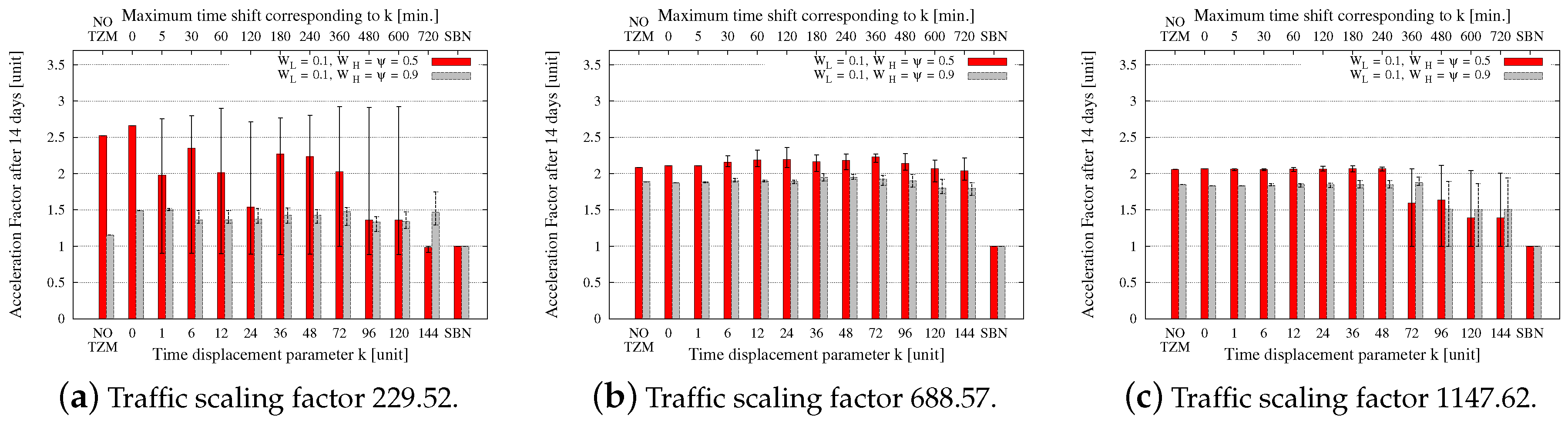Figure 10 reports the obtained results in terms of $A{F}_{avg}$ over all LCs in the network after 14 days of network operation. In both cases, averages over all considered SVMs are reported (bar plots) and complemented with the maximum and minimum values (error bars).

Interestingly, it is possible to save energy for most values of the time displacement parameter k. This can be clearly observed in the case of a scaling factor 688.57 (Figure 9b). Average energy consumption increases when traffic is scaled with the factor 1147.62 and when k becomes high (Figure 9c). This is caused by the existence of multiple shortest paths between some node pairs. In particular, EWA sometimes finds other shortest paths than the ones used in the SBN and therefore occasionally has problems with satisfying all the traffic demands. We have verified that unsatisfied demands never exceed 6%. EWA does not put LCs into SM in such cases, and therefore energy consumption is identical with that in the SBN (compare SBN in Figure 9c with the maximum energy consumption values for $k\ge$ 72). This effect of occasional routing incompatibilities is even stronger when the scaling factor is low (see high and intermediate values of k in Figure 9a). On the contrary, it is always possible to save energy when no TZM is used and when k is equal to 0, i.e., when all demands have an off-peak zone occurring during the same hours (cf. Figure 2a) or when the peak times only depend on the time zone where nodes are located.

Considering $A{F}_{avg}$ (Figure 10), it is interesting to note that these figures are complementary to the energy figures, i.e., the lower the energy consumption, the higher the AF. $A{F}_{avg}$ usually takes values between 1.2 and 2.5 meaning that energy saving reduces devices lifetime. For the cases in which EWA encounters routing incompatibilities, $A{F}_{avg}$ decreases. This happens more frequently with increasing k. In the cases when most LCs are constantly powered on (i.e., the energy consumption of the network using EWA is close to the one of the SBN), few power state reconfigurations are introduced, resulting in an AF close to 1 (see, e.g., the case for $k=144$ in Figure 10a for $W_L=0.1$ and $W_H=\psi =0.5$).

6.3. Influence of HW Parameters

In the following, we vary the HW parameters $A{F}^{sleep}$ and χ, which are used in the computation of the AF of the LCs. Specifically, since EWA does not consider the lifetime of the LCs to take power state decisions, the variation of such parameters has no influence on the total energy consumption $E_{total}^{EWA}$. On the contrary, the experienced LCs lifetime is heavily impacted by the variation of $A{F}^{sleep}$ and χ, as reported in Figure 11. Clearly, the frequency of AM-SM-AM cycles χ significantly affects the results. For example, when χ is varied and $A{F}^{sleep}=0.5$, $A{F}_{avg}$ falls in the ranges 2.52–17.67, 2.08–14.23, and 2.06–14.21 units for the scaling factors 229.52, 688.57, and 1147.62 respectively. On the other hand, the influence of $A{F}^{sleep}$ on $A{F}_{avg}$ is minor. When $\chi =0.5$ h/cycle and $A{F}^{sleep}$ is varied, $A{F}_{avg}$ falls in the ranges 2.42–2.62, 1.92–2.24, and 1.88–2.23 units for the scaling factors 229.52, 688.57, and 1147.62 respectively.

6.4. Evaluation of Network Profitability

Finally, we analyze the results in terms of network profitability $R_{total}$ as reported in Figure 12. Positive values indicate that monetary energy saving due to the dynamic usage of SM is higher than the corresponding reparation costs. Interestingly, $R_{total}>0$ in most of the cases. In particular, the profitability increases when the network load is increased (see e.g., the increasing range of the y-scale across Figure 12a–c). A negative profitability (i.e., a cost for the operator) is observed only in the case when $A{F}^{sleep}=0.5$ and $\chi =5.0$. This is the worst assumption for the usage of SM, i.e., $A{F}^{sleep}=0.5$ represents the lowest benefit for the LC lifetime due to putting it into SM, and $\chi =5.0$ means the highest penalty for the LC lifetime due to the state transition. In this case, the application of SM leads to high reparation costs, which are even higher than the achieved energy savings.

7. Conclusions

We have proposed a simple traffic model covering both temporal and spatial traffic variations. The model has been realistically parametrized and used to generate sets of traffic matrices. These traffic matrices have been used as input for running the energy-aware approach EWA, which determines the set of LCs to be put into SM during network operation.

Our results, obtained from a realistic scenario, confirm the strong influence of temporal traffic variation on energy consumed by LCs in the network. In contrast to this aspect, the pace of traffic variation has a limited impact on energy consumption and no impact on devices lifetime according to our model. Furthermore, our evaluation shows that energy savings are possible when traffic varies over space. Moreover, application of EWA leads in general to a reduction of LCs lifetime, as a consequence of the different power state transitions introduced by this energy-aware approach. However, positive profitability is achieved in most of the cases.

As future work, we plan to vary network topologies as well as network design methods to avoid routing incompatibilities. Furthermore, we are going to consider alternative heuristics for dynamic network operation to directly target QoS, devices lifetime, and profitability when making decisions about which LCs to put into SM and which ones to keep active. Eventually, variation of different sets of parameters in the proposed traffic model is a step towards reality despite the complexity of its influence on results.

References

1. Zhang, Y.; Chowdhury, P.; Tornatore, M.; Mukherjee, B. Energy Efficiency in Telecom Optical Networks. IEEE Commun. Surv. Tutor. 2010, 12, 441–458. [Google Scholar] [CrossRef]
2. Idzikowski, F.; Chiaraviglio, L.; Cianfrani, A.; López Vizcaíno, J.; Polverini, M.; Ye, Y. A Survey on Energy-Aware Design and Operation of Core Networks. IEEE Commun. Surv. Tutor. 2016, 18, 1453–1499. [Google Scholar] [CrossRef]
3. Chiaraviglio, L.; Wiatr, P.; Monti, P.; Chen, J.; Lorincz, J.; Idzikowski, F.; Listanti, M.; Wosinska, L. Is green networking beneficial in terms of device lifetime? IEEE Commun. Mag. 2015, 53, 232–240. [Google Scholar] [CrossRef]
4. Lange, C.; Gladisch, A. Energy efficiency limits of load adaptive networks. In Proceedings of the 2010 Conference on Optical Fiber Communication (OFC), Collocated National Fiber Optic Engineers Conference, San Diego, CA, USA, 21–25 March 2010.
5. Lange, C.; Gladisch, A. Limits of Energy Efficiency Improvements by Load-Adaptive Telecommunication Network Operation. In Proceedings of the 10th Conference of Telecommunication, Media and Internet Techno-Economics (CTTE), Berlin, Germany, 16–18 May 2011.
6. Idzikowski, F.; Pfeuffer, F.; Werner, A.; Chiaraviglio, L. Impact of Spatial Traffic Variation on Energy Savings and Devices Lifetime in Core Networks. In Proceedings of the 2016 IEEE 17th International Conference on High Performance Switching and Routing (HPSR), Yokohama, Japan, 14–17 June 2016.
7. Almeida, S.; Queijo, J.; Correia, L.M. Spatial and temporal traffic distribution models for GSM. In Proceedings of the 1999 Fall IEEE VTS 50th Vehicular Technology Conference, Amsterdam, The Netherlands, 19–22 September 1999.
8. Lee, D.; Zhou, S.; Zhong, X.; Niu, Z.; Zhou, X.; Zhang, H. Spatial modeling of the traffic density in cellular networks. IEEE Wirel. Commun. 2014, 21, 80–88. [Google Scholar] [CrossRef]
9. Wu, Y.; Min, G.; Li, K.; Javadi, B. Modeling and Analysis of Communication Networks in Multicluster Systems under Spatio-Temporal Bursty Traffic. IEEE Trans. Parallel Distrib. Syst. 2012, 23, 902–912. [Google Scholar] [CrossRef]
10. Coiro, A.; Iervini, F.; Listanti, M. Distributed and Adaptive Interface Switch Off for Internet Energy Saving. In Proceedings of the 20th International Conference on Computer Communications and Networks (ICCCN), New Delhi, India, 31 July–4 August 2011.
11. Coiro, A.; Listanti, M.; Valenti, A. Impact of Energy-Aware Topology Design and Adaptive Routing at Different Layers in IP over WDM networks. In Proceedings of the XVth International Telecommunications Network Strategy and Planning Symposium (NETWORKS), Rome, Italy, 15–18 October 2012.
12. Coiro, A.; Listanti, M.; Valenti, A.; Matera, F. Energy-aware traffic engineering: A routing-based distributed solution for connection-oriented IP networks. Comput. Netw. 2013, 57, 2004–2020. [Google Scholar] [CrossRef]
13. Chiaraviglio, L.; Mellia, M.; Neri, F. Energy-aware Backbone Networks: A Case Study. In Proceedings of the 2009 IEEE International Conference on Communications Workshops, Dresden, Germany, 14–18 June 2009.
14. Scharf, J. Efficiency Analysis of Distributed Dynamic Optical Bypassing Heuristics. In Proceedings of the 2012 IEEE International Conference on Communications (ICC), Ottawa, ON, Canada, 10–15 June 2012.
15. Lui, Y.; Shen, G.; Shao, W. Optimal Port Grouping for Maximal Router Card Sleeping. In Proceedings of the 2012 Asia Communications and Photonics Conference (ACP), Guangzhou, China, 7–10 November 2012.
16. Lui, Y.; Shen, G.; Bose, S.K. Energy-Efficient Opaque IP over WDM Networks with Survivability and Security Constraints. In Proceedings of the 2013 Asia Communications and Photonics Conference, Beijing, China, 12–15 November 2013.
17. Lui, Y.; Shen, G.; Shao, W. Design for Energy-Efficient IP Over WDM Networks With Joint Lightpath Bypass and Router-Card Sleeping Strategies. J. Opt. Commun. Netw. 2013, 5, 1122–1138. [Google Scholar] [CrossRef]
18. Chiaraviglio, L.; Mellia, M.; Neri, F. Reducing Power Consumption in Backbone Networks. In Proceedings of the 2009 IEEE International Conference on Communications (ICC), Dresden, Germany, 14–18 June 2009.
19. Bianzino, A.P.; Chaudet, C.; Moretti, S.; Rougier, J.L.; Chiaraviglio, L.; Le Rouzic, E. Enabling Sleep Mode in Backbone IP-Networks: A Criticality-Driven Tradeoff. In Proceedings of the 2012 IEEE International Conference on Communications, Ottawa, ON, Canada, 10–15 June 2012.
20. Bianzino, A.P.; Chiaraviglio, L.; Mellia, M. GRiDA: A Green Distributed Algorithm for Backbone Networks. In Proceedings of the 2011 IEEE Online Conference on Green Communications (GreenCom), New York, NY, USA, 26–29 September 2011.
21. Bianzino, A.P.; Chiaraviglio, L.; Mellia, M.; Rougier, J.L. GRiDA: GReen Distributed Algorithm for energy-efficient IP backbone networks. Comput. Netw. 2012, 56, 3219–3232. [Google Scholar] [CrossRef]
22. Tego, E.; Idzikowski, F.; Chiaraviglio, L.; Coiro, A.; Matera, F. Facing the reality: Validation of energy saving mechanisms on a testbed. J. Electr. Comput. Eng. 2014, 2014, 1–11. [Google Scholar] [CrossRef]
23. Dong, X.; El-Gorashi, T.; Elmirghani, J. Hybrid-power IP over WDM network. In Proceedings of the 2010 Seventh International Conference On Wireless And Optical Communications Networks (WOCN), Colombo, Sri Lanka, 6–8 September 2010.
24. Dong, X.; El-Gorashi, T.; Elmirghani, J. IP over WDM Networks Employing Renewable Energy Sources. J. Lightwave Technol. 2011, 29, 3–14. [Google Scholar] [CrossRef]
25. Dong, X.; El-Gorashi, T.; Elmirghani, J. Energy Efficient Optical Networks with Minimized Non-Renewable Power Consumption. J. Netw. 2012, 7, 821–831. [Google Scholar] [CrossRef]
26. Dong, X.; El-Gorashi, T.; Elmirghani, J. Energy-Efficient IP over WDM Networks with Data Centres. In Proceedings of the 2011 13th International Conference on Transparent Optical Networks (ICTON), Stockholm, Sweden, 26–30 June 2011.
27. Dong, X.; El-Gorashi, T.; Elmirghani, J. Green IP Over WDM Networks With Data Centers. J. Lightwave Technol. 2011, 29, 1861–1880. [Google Scholar] [CrossRef]
28. Dong, X.; Lawey, A.; El-Gorashi, T.; Elmirghani, J. Energy-Efficient Core Networks. In Proceedings of the 2012 16th International Conference on Optical Network Design and Modeling (ONDM), Colchester, UK, 17–20 April 2012.
29. Dong, X.; El-Gorashi, T.; Elmirghani, J. On the Energy Efficiency of Physical Topology Design for IP Over WDM Networks. J. Lightwave Technol. 2012, 30, 1931–1942. [Google Scholar] [CrossRef]
30. Mukherjee, B. Optical WDM Networks; Springer: New York, NY, USA, 2006. [Google Scholar]
31. Betker, A.; Gamrath, I.; Kosiankowski, D.; Lange, C.; Lehmann, H.; Pfeuffer, F.; Simon, F.; Werner, A. Comprehensive Topology and Traffic Model of a Nationwide Telecommunication Network. J. Opt. Commun. Netw. 2014, 6, 1038–1047. [Google Scholar] [CrossRef]
32. Ahmad, A.; Bianco, A.; Bonetto, E.; Chiaraviglio, L.; Idzikowski, F. Energy-Aware Design of Multi-layer Core Networks. J. Opt. Commun. Netw. 2013, 5, A127–A143. [Google Scholar] [CrossRef]
33. Bonetto, E.; Chiaraviglio, L.; Idzikowski, F.; Le Rouzic, E. Algorithms for the Multi-Period Power-Aware Logical Topology Design with Reconfiguration Costs. J. Opt. Commun. Netw. 2013, 5, 394–410. [Google Scholar] [CrossRef]
34. Idzikowski, F.; Bonetto, E.; Chiaraviglio, L. EWA—An Adaptive Algorithm Using Watermarks for Energy Saving in IP-Over-WDM Networks; Technical Report TKN-12-002; Technische Universität Berlin: Berlin, Germany, 2012. [Google Scholar]
35. Zhang, Y. 6 Months of Abilene Traffic Matrices. Available online: http://www.cs.utexas.edu/~yzhang/research/AbileneTM/ (accessed on 13 October 2016).
36. Zuse Institut Berlin. Library of test instances for Survivable fixed telecommunication Network Design. Available online: http://sndlib.zib.de/home.action (accessed on 13 October 2016).
37. Idzikowski, F.; Chiaraviglio, L.; Portoso, F. Optimal Design of Green Multi-layer Core Networks. In Proceedings of the 2012 Third International Conference on Future Energy Systems: Where Energy, Computing and Communication Meet (e-Energy), Madrid, Spain, 9–11 May 2012.
38. Hülsermann, R.; Gunkel, M.; Meusburger, C.; Schupke, D.A. Cost Modeling and Evaluation of Capital Expenditures in Optical Multilayer Networks. J. Opt. Netw. 2008, 7, 814–833. [Google Scholar] [CrossRef]
39. Van Heddeghem, W.; Idzikowski, F. Equipment Power Consumption in Optical Multilayer Networks—Source Data; Technical Report IBCN-12-001-01; Ghent University: Ghent, Belgium, 2012. [Google Scholar]
40. Zhang, Y.; Tornatore, M.; Chowdhury, P.; Mukherjee, B. Energy optimization in IP-over-WDM networks. Opt. Switch. Netw 2011, 8, 171–180. [Google Scholar] [CrossRef]
41. Arrhenius, S. Über die Reaktionsgeschwindigkeit Bei der Inversion von Rohrzucker Durch Säuren; Wilhelm Engelmann: Leipzig, Germany, 1889. [Google Scholar]
42. Wiatr, P.; Chen, J.; Monti, P.; Wosinska, L. Energy Efficiency versus Reliability Performance in Optical Backbone Networks. J. Opt. Commun. Netw. 2015, 7, A482–A491. [Google Scholar] [CrossRef]
43. European Commission. Energy Prices and Costs Report. Available online: http://ec.europa.eu/energy/sites/ener/files/documents/20140122_swd_prices.pdf (accessed on 13 October 2016).
44. Cisco ONS 15454 Multiservice Transport Platform—MSTP. Available online: http://www.cisco.com/c/en/us/products/optical-networking/ons-15454-multiservice-transport-platform-mstp/index.html (accessed on 16 August 2016).
45. Wiatr, P.; Chen, J.; Monti, P.; Wosinska, L. Energy saving in access networks: Gain or loss from the cost perspective? In Proceedings of the 2013 15th International Conference on Transparent Optical Networks (ICTON), Cartagena, Spain, 23–27 June 2013.
46. IBM–ILOG. Cplex 12.6.0. Available online: http://www.ibm.com/software/commerce/optimization/cplex-optimizer/ (accessed on 13 October 2016).
47. Pióro, M.; Medhi, D. Routing, Flow, and Capacity Design in Communication and Computer Networks; Morgan Kaufmann Publishers: San Mateo, CA, USA, 2004. [Google Scholar]
Figure 1. Temporal traffic model with exemplary relative demand values and even number of elements in the set of time periods T covering a day.
Energies 09 00837 g001
Figure 2. Example for the spatial variation of traffic demands—total network traffic (red) and single demand curves (black) for granularity Δ t = 1 h and different values of the displacement parameter k in a three-node network.
Energies 09 00837 g002
Figure 3. Energy consumption E t o t a l E W A over a day vs. the ratio A m i n a , b / A m a x a , b .
Energies 09 00837 g003
Figure 4. A F a v g with A F s l e e p = 0.5 units and χ = 0.5 h/cycle after 14 days vs. the ratio A m i n a , b / A m a x a , b .
Energies 09 00837 g004
Figure 5. Energy consumption E t o t a l E W A over a day vs. the length of T l o w .
Energies 09 00837 g005
Figure 6. A F a v g with A F s l e e p = 0.5 units and χ = 0.5 h/cycle after 14 days vs. the length of T l o w .
Energies 09 00837 g006
Figure 7. Energy consumption E t o t a l E W A over a day vs. the ratio A m i n a , b / A m a x a , b with fixed total load.
Energies 09 00837 g007
Figure 8. A F a v g with A F s l e e p = 0.5 units and χ = 0.5 h/cycle after 14 days vs. the ratio A m i n a , b / A m a x a , b with fixed total load.
Energies 09 00837 g008
Figure 9. Average energy consumed by all LCs over a day over all SVMs in the Abilene-based network using two EWA settings. The error bars indicate the minimum and maximum values over all SVMs.
Energies 09 00837 g009
Figure 10. A F a v g over all LCs (after 14 days) and over all SVMs in the Abilene-based network using two EWA settings. The error bars indicate the minimum and maximum values over all SVMs.
Energies 09 00837 g010
Figure 11. AF after 14 days vs. the HW parameters with | T l o w | = 72, | T i n c | = 36.
Energies 09 00837 g011
Figure 12. Profitability R t o t a l after 14 days vs. the HW parameters with | T l o w | = 72, | T i n c | = 36.
Energies 09 00837 g012