Revenue Risk of U.S. Tight-Oil Firms

Abstract

American U.S. crude oil prices have dropped significantly of late down to a low of less than $30 a barrel in early 2016. At the same time price volatility has increased and crude in storage has reached record amounts in the U.S. America. Low oil prices in particular pose quite a challenge for the survival of U.S. America’s tight-oil industry. In this paper we assess the current profitability and future prospects of this industry. The question could be broadly stated as: should producers stop operation immediately or continue in the hope that prices will rise in the medium term? Our assessment is based on a stochastic volatility model with three risk factors, namely the oil spot price, the long-term oil price, and the spot price volatility; we allow for these sources of risk to be correlated and display mean reversion. We then use information from spot and futures West Texas Intermediate (WTI) oil prices to estimate this model. Our aim is to show how the development of the oil price in the future may affect the prospective revenues of firms and hence their operation decisions at present. With the numerical estimates of the model’s parameters we can compute the value of an operating tight-oil field over a certain time horizon. Thus, the present value (PV) of the prospective revenues up to ten years from now is $37.07/bbl in the base case. Consequently, provided that the cost of producing a barrel of oil is less than $37.07 production from an operating field would make economic sense. Obviously this is just a point estimate. We further perform a Monte Carlo (MC) simulation to derive the risk profile of this activity and calculate two standard measures of risk, namely the value at risk (VaR) and the expected shortfall (ES) (for a given confidence level). In this sense, the PV of the prospective revenues will fall below $22.22/bbl in the worst 5% of the cases; and the average value across these worst scenarios is $19.77/bbl. Last we undertake two sensitivity analyses with respect to the spot price and the long-term price. The former is shown to have a stronger impact on the field’s value than the latter. This bodes well with the usual time profile of tight oil production: intense depletion initially, followed by steep decline thereafter.

1. Introduction

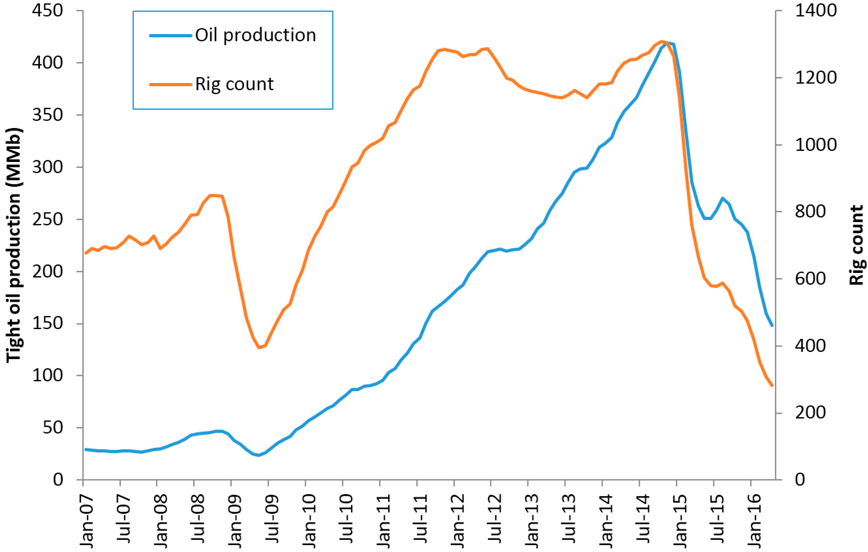
Starting in the 1970s U.S. oil production has witnessed a long period of decline. This phase came to an end in early 2008 [1]. As shown in Figure 1, from then on domestic oil production increased significantly. This increase can be explained to a large extent by the exploitation of geological formations that are characterized by low porosity and extremely low permeability [2,3,4]. In this regard, tight oil is a broader term than shale oil in that it can be extracted from shale beds or other low-permeability reservoirs (e.g., limestone, sandstone).

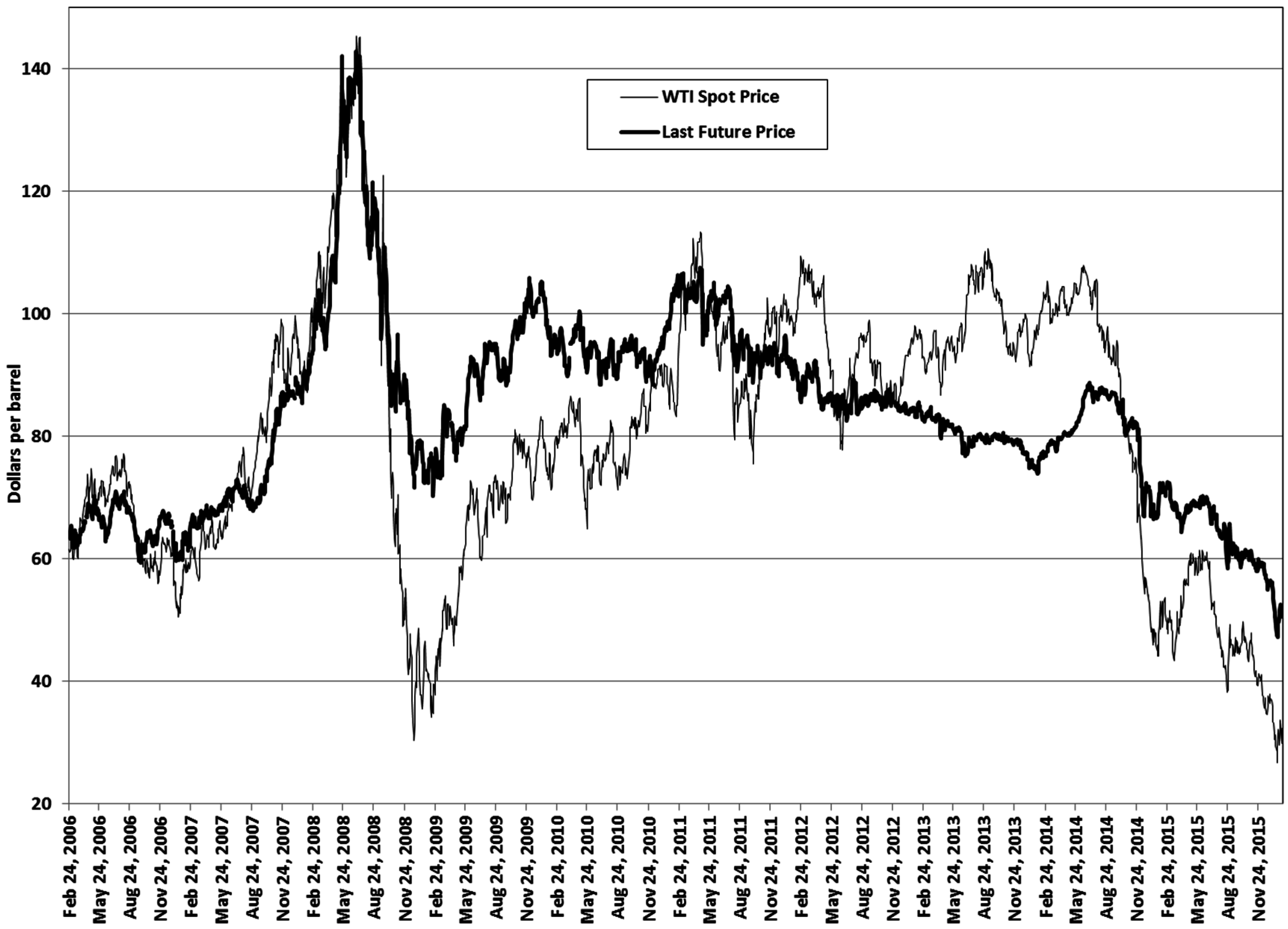
Until recently production of these diffuse, unconventional fossil resources was considered uneconomic, but the successful combination of horizontal drilling and hydraulic fracturing (or fracking) during the last decade has brought vast amounts of shale gas and tight oil that were previously inaccessible within reach [5]. At the same time, West Texas Intermediate (WTI) oil prices were at relatively high levels; see Figure 2 (prices from the Intercontinental Exchange, ICE).

Note that the economics of tight oil production is different from that of conventional oil extraction: (a) quick ramp-up periods that make it easier to meet expected increases in market demand; (b) small upfront investment outlay; (c) high initial decline rates (65%–80% in first year); (d) low lifting costs; and (e) only two-three years of hedge-ability are needed. Successful hedging in particular is vital to mitigating falling prices [6].

Certainly, as both technology and operator experience mature tight oil can be extracted at higher efficiency levels. Productivity improvements in turn imposed a downward pressure on the wellhead break-even oil price, which has decreased by more than 40% across all main shale plays in North America between 2013 and 2015 [7]. Nonetheless, in view of the decline in crude oil prices that began in the summer of 2014, strong prices can no longer be taken for granted. In fact, now output has begun to fall, especially among high-cost producers [8].

This paper focuses on the prospects for U.S. producers of tight oil. Their net income obviously depends on both revenues and costs. It is hard to get good cost data. This is partly because of limited information available about: (i) the rate at which tight-oil wells become less productive over time; and (ii) the distribution of well productivity [9]. We pay special attention to revenues. From this viewpoint, the future behavior of the crude oil price is paramount: it determines when production is profitable [10].

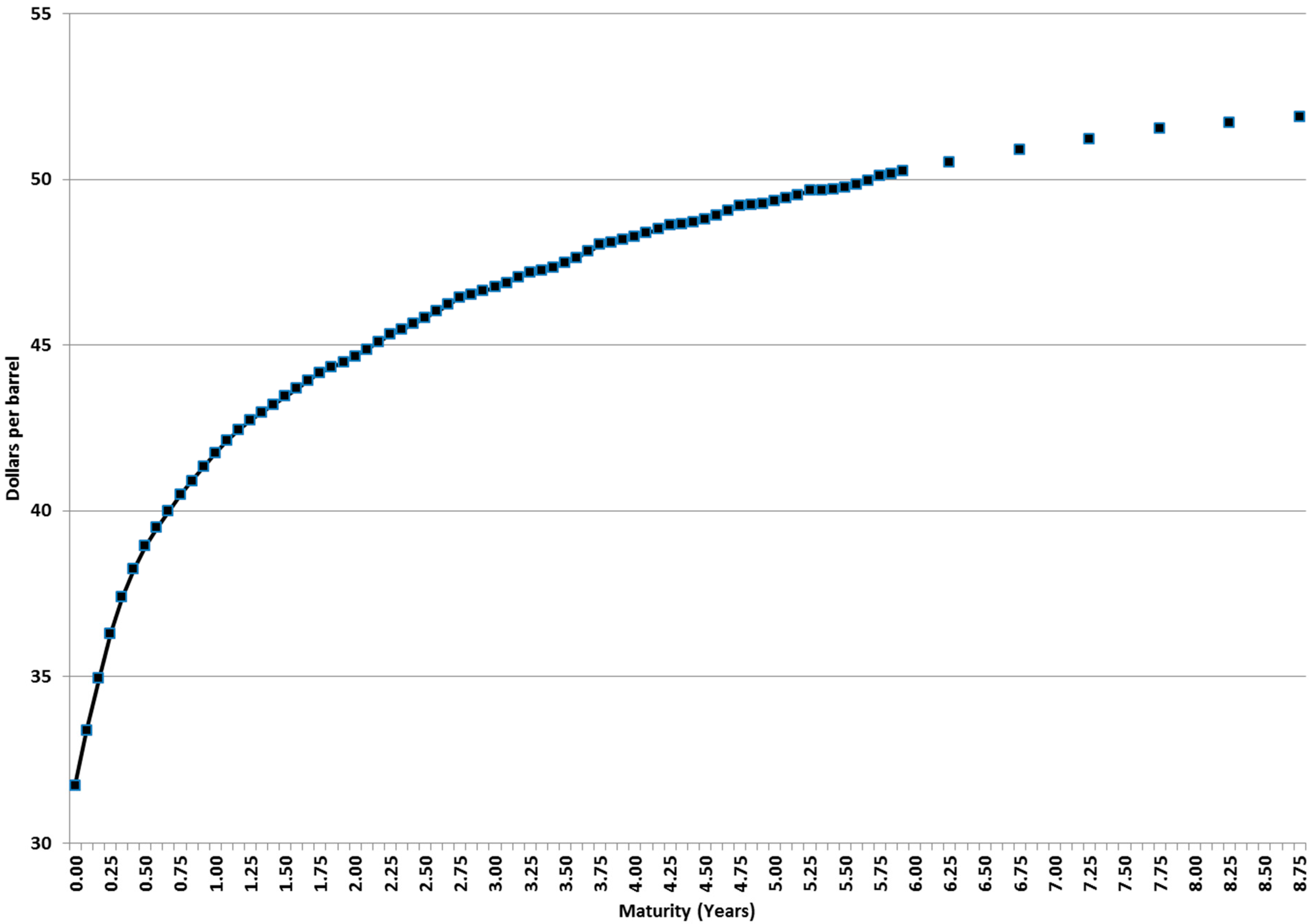
Lower oil prices could be anticipated to negatively impact production rates [11]. Yet the effect on the U.S. tight-oil sector has been far from immediate; see Figure 1. At the same time, the shale industry is assumed to be able to increase production quickly, once it becomes profitable to do so. Therefore, an eventual price recovery would likely promote the resumption of output from many areas [12]. Indeed, the curve of oil futures prices shows an increasing profile; see Figure 3. Thus, in principle producers could wait for higher prices before resuming operations while selling their output at oil prices above $40/bbl for future delivery (as of mid-May 2016 spot prices edged towards $50/bbl).

The oil price above which tight-oil producers can resume drilling and make money again is a crucial issue in this paper (similarly for the production cost below which operation is worthwhile). This threshold or “break-even” level is not only paramount for the producers involved. Depending on its level the consequences could be felt way beyond the shale beds and reach the whole economy as it could fundamentally alter the entire dynamics of the oil market.

To our knowledge, there is no academic or scientific literature that addresses this specific issue. The topic is pursued in several reports from industry outfits and government agencies. At this point, however, an important remark is in order; it concerns the precise definition of the break-even itself. For example, in [13] the break-even WTI price is defined as the price at which a producer will hit a pre-specified after-tax internal rate of return (10% and 20%). The limitations and shortcomings of the internal rate of return as an investment criterion are well known; see for instance [14]. And the adoption of a particular target level (say, 20%) in the absence of a full-fledged valuation model is a bit ad hoc. The break-even oil price is certainly the usual metrics for assessing profitability; see [9,15]. Similarly, all break-evens in [16] are calculated by finding the oil price that makes the net present value (NPV) of the field equal to zero. The NPV strongly depends on the discount rate applied, which reflects the oil firms’ profit requirements (a 10% rate is used). However, sometimes the break-even cost is invoked too; see [17]. Our definition goes along this line: when addressing the valuation of an operating tight-oil well, our “break-even” is the (unit) cost (here assumed deterministic) that makes that specific well's NPV drop to zero as seen from today (see Section 5 below). Besides, since we adopt risk-neutral valuation, the precise discount rate is hardly arbitrary: based on sound financial principles, it must be the riskless interest rate.

In what follows we focus on operating wells. We leave aside the financial condition of tight-oil producers, their levels of debt, whether they are cash strapped, etc. It may well be quite rational to keep producing at oil prices below the break-even, for example to maintain cash flow and service debt, or to avoid the costs associated with closure, financial distress costs, or others. Reference [18] considers how companies are going to be able to implement strategies to address their debt loads.

We propose a model in which the spot price of oil evolves stochastically over time while displaying mean reversion. The volatility of price changes is similarly assumed to be stochastic and mean reverting. As for the long-term price (toward which the spot price tends to revert), in principle it can be correlated with the spot price and, consequently, show mean reversion too. We then estimate the model with daily prices of the ICE WTI Light Sweet Crude Oil Futures Contract traded on the ICE.

By drawing on futures prices we can undertake so-called risk-neutral valuation. Hence we develop a model for the (gross) value of an operating tight-oil field (we restrict ourselves to considering cash inflows); for convenience we express this value in per-unit terms, i.e., per barrel of initial reserves. Our numerical parameter estimates are applied to this valuation model over a given time horizon (10 years). Thus we can compute the present value (PV) of the revenues to be collected over the valuation horizon. Interestingly this PV can be interpreted as a “trigger” or “break even” level for oil producers: a cost (per barrel) above this cumulative inflow of cash will translate into a NPV with its ensuing consequences. When we refer to costs we mean costs not incurred yet, i.e., the costs to be met in the future. The point here is whether the oil company will make a profit by producing from now onwards (this is the right approach even though the process as a whole from the beginning may be unprofitable). In addition, we assess the (revenue) risk faced by these producers. Specifically, we run a number of Monte Carlo (MC) simulations to derive the probability distribution of the PV of an oil well’s revenues. We synthesize this information into a pair of measures of risk, namely the value at risk (VaR) and the expected shortfall (ES) for the standard confidence level (95%). We finally check the robustness of our results with respect to changes in the spot price and the long-term future price.

The paper is organized as follows: after this Introduction, Section 2 develops the theoretical model for crude oil price; our data sample is described in Section 3, followed by the econometric analysis in Section 4; we then move to the valuation of a tight-oil field in Section 5; Section 6 presents our major results in terms of the revenue risk faced by U.S. producers; Section 7 includes some sensitivity analyses; lastly, Section 8 presents our conclusions.

2. Stochastic Model for Crude Oil Price

Early analyses that considered oil price as a stochastic process adopted the geometric Brownian motion (GBM); see for instance [19,20]. Subsequent one-factor diffusion models typically displayed mean reversion, e.g., the Ornstein–Uhlenbeck process in [21]. More sophisticated two- and three-factor diffusion models can be found in [22,23,24,25,26], among others. In some of these models the commodity price follows a standard GBM while the interest rate and/or the convenience yield show mean reversion. Here we develop a stochastic model with three sources of risk. We consider a stochastic long-term price alongside the spot price and the stochastic volatility. This is because the long-term price changes over time and is a key factor for evaluating long-run investments and risks. Oil price tends toward a long-term level that is determined by futures prices of contracts with distant maturities. And the volatility of price changes is mean-reverting too. Specifically:

$$\mathrm{d}{S}_t=\left[k(S_t^m-S_t)-\mathsf{\lambda }{S}_t\right]\mathrm{d}t+{\mathsf{\sigma }}_t{S}_t\mathrm{d}{W}^1$$

(1)

$$\mathrm{d}{S}_t^{*}=\mathsf{\upsilon }{S}_t^{*}\mathrm{d}{W}^2$$

(2)

$${\mathrm{d}\mathsf{\sigma }}_t={\mathsf{\nu }(\mathsf{\sigma }}^{*}-{\mathsf{\sigma }}_t)\mathrm{d}t+{\mathsf{\varsigma }\mathsf{\sigma }}_t\mathrm{d}{W}^3$$

(3)

$$E(\mathrm{d}{W}^1,\mathrm{d}{W}^2)={\mathsf{\rho }}_{1,2}\mathrm{d}t;E(\mathrm{d}{W}^1,\mathrm{d}{W}^3)={\mathsf{\rho }}_{1,3}\mathrm{d}t;E(\mathrm{d}{W}^2,\mathrm{d}{W}^3)={\mathsf{\rho }}_{2,3}\mathrm{d}t$$

(4)

We assume that the time-t (spot) crude oil price, S_t, evolves stochastically in the risk-neutral world according to a mean-reverting process like the inhomogeneous (or integrated) geometric Brownian motion, or IGBM for short ([27,28,29,30]). In Equation (1), $S_t^m$ stands for the long-term equilibrium level towards which S_t tends to revert in the physical, real world with the passage of time. k is the speed of reversion; it determines how quickly the expected value of oil price E[S_t] approaches the long-term equilibrium level. λ stands for the market price of risk. σ_t is the instantaneous volatility of oil price changes. And $\mathrm{d}{W}^1={\mathsf{\epsilon }}_t^1\sqrt{\mathrm{d}t}$ is the increment to a standard Wiener process where ${\mathsf{\epsilon }}_t^1:N(0,1)$. Equation (1) can be equivalently rewritten as:

$$\mathrm{d}{S}_t=(k+\mathsf{\lambda })(S_t^{*}-S_t)\mathrm{d}t+{\mathsf{\sigma }}_t{S}_t\mathrm{d}{W}^1$$

(5)

Here, $S_t^{*}\equiv \frac{k{S}_t^m}{k+\mathsf{\lambda }}$ denotes the corresponding long-term level in the risk neutral world (this applies too in futures markets).

As shown in Equation (2), we assume that $S_t^{*}$ is not deterministic but changes stochastically, unpredictably over time with instantaneous volatility υ. Though at time t we cannot predict its level at a future date T, it can be proven that $E_t(S_T^{*})=S_t^{*}$, i.e., the expected value can be inferred from the current curve of crude oil prices in the futures markets on any particular day (e.g., the last sample day). Thus, what we know about $S_t^{*}$ is only its expected value and the volatility.

Regarding the IGBM in Equation (3), we further assume that oil price volatility σ_t displays mean reversion. σ* denotes the long-term equilibrium level towards which σ_t tends to revert in the long term. It does so at speed ν, which determines how fast E(σ_t) approaches σ*. And ς denotes a scaling factor for the volatility. In the area of stochastic volatility models, the IGBM is called the GARCH diffusion model in [31]. Indeed, the version of the IGBM process in discrete time is just the GARCH(1,1) model.

As for Equation (4), in principle the three stochastic processes can be correlated. Whether in reality they are or not is an empirical issue. We will touch upon this issue in Section 4. At this point we merely observe that the long-term price $S_t^{*}$ follows a random walk but, since it is correlated with S_t (via ρ₁₂), in practice it behaves as a mean-reverting process.

Now, reference [32] shows that, in the risk-neutral world (under the equivalent martingale measure or risk-neutral probability measure P), the time-t expected value of the spot price at T, or equivalently the futures price for maturity T, is given by:

$$E_t^P(S_T)=F(t,T)=S_t^{*}+[S_t-S_t^{*}]{\mathrm{e}}^{-(k+\mathsf{\lambda })(T-t)}$$

(6)

Note that the price change volatility σ_t has no impact on this expectation. A similar argument can be made for the futures contract with the nearest maturity, T₁, to estimate the futures price with maturity T₂:

$$F(t,T_2)=S_t^{*}+[F(t,T_1)-S_t^{*}]{\mathrm{e}}^{-(k+\mathsf{\lambda })(T_2-T_1)}$$

(7)

Equation (7) allows us to estimate daily values of $S_t^{*}\equiv \frac{k{S}_t^m}{k+\mathsf{\lambda }}$ and k + λ from observed daily futures prices by non-linear least squares. On the other hand, the long-term equilibrium level on the futures market is given by:

$$F(t,\infty )=\frac{k{S}_m}{k+\mathsf{\lambda }}\equiv S_t^{*}$$

(8)

3. Sample Data

The ICE WTI Light Sweet Crude Oil Futures Contract is traded on the ICE, an electronic marketplace. The contract size is 1000 barrels. The units of trading are any multiple of this amount. The contracts listed cover up to 108 consecutive months. Prices are quoted in US dollars and cents. The contract is settled in cash against the prevailing market price for US light sweet crude. Financial performance of all ICE Futures Europe contracts are guaranteed by ICE Clear Europe provided they are registered with it by its clearing Members. Note that oil futures prices can well be different in other major markets, e.g., the New York Mercantile Exchange (NYMEX), but arbitrage-based arguments pose severe restrictions on the potential price gaps; in other words, the differences in prices should be small.

Our sample consists of 161,274 daily futures prices. The time span ranges from 24 February 2006 to 4 February 2016, i.e., almost ten years. We first classify the data according to the contract’s time to maturity (T).

Table 1. Volatility of some futures contracts according to their maturity.

Maturity	# Observations	Return Volatility
Nearest (1 month)	2571	0.3175
6 months	2571	0.2859
12 months	2571	0.2602
18 months	2571	0.2452
24 months	2571	0.2324
30 months	2548	0.2250
36 months	2420	0.2201
42 months	2246	0.2176
48 months	2189	0.2155

shows the number of observations and the return volatility of some futures contracts in our sample.

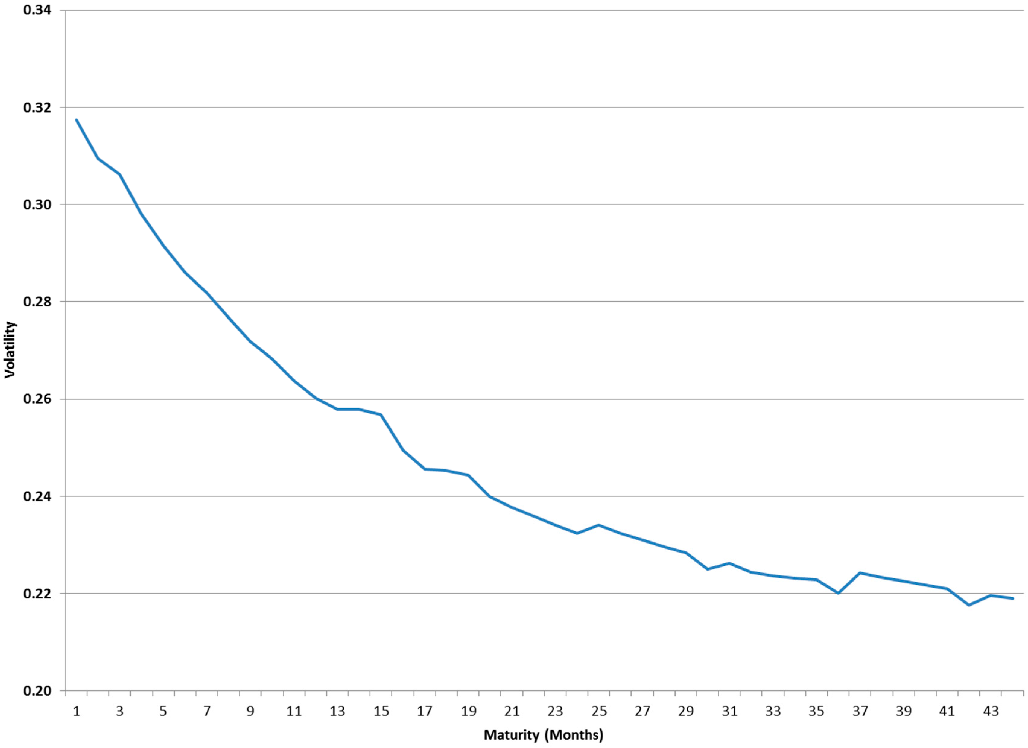
We can observe that futures contracts with longer times to expiration (T − t) display lower return volatilities (this is the so-called Samuelson effect). Figure 4 displays this behavior. Consistent with this pattern, as a particular contract approaches its maturity and T − t decreases (a leftward movement in Figure 4) volatility increases and the futures price converges toward the spot price, so that F(T,T) = S_T.

4. Econometric Analysis

We initially compute the values of k + λ and $S_t^{*}$ (see Equations (1) and (5)) on each day using non-linear least squares. Thus, for example, since we have 2571 prices of the nearest-to-maturity futures contracts we estimate 2571 values for each parameter. We are interested in getting a numerical estimate of the volatility υ in Equation (2). Nonetheless, a few outliers are identified in the original time series of ${\left\{S_t^{*}\right\}}_{t\ge 0}$ so we filter them out following the procedure described in the Appendix A. With the new, filtered series of long-term prices we calculate a volatility υ = 0.2477.

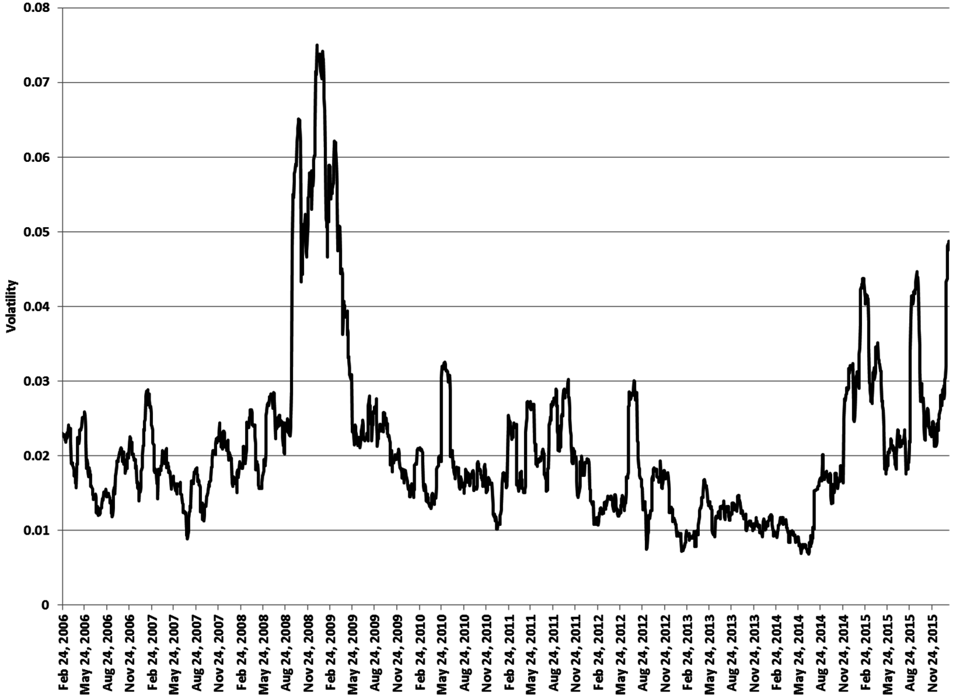
Regarding the spot price volatility σ_t (see Equations (1), (3) and (5)) we adopt the following approach (the Appendix A sheds more light on this issue). We first note that it is not constant; see Figure 5. Here, on any sample day we take the return on that particular day and those on the previous 24 days. We compute the standard deviation over these 25 days. We then multiply this daily volatility times the square root of 252 so as to get a yearly volatility.

Using the volatility series {σ_t}_t≥0 calculated with a 25-day moving window we estimate the following model:

$$\frac{{\mathsf{\sigma }}_{t+\Delta t}-{\mathsf{\sigma }}_t}{{\mathsf{\sigma }}_t}=-\nu \Delta t+\nu {\mathsf{\sigma }}^{*}\Delta t\frac{1}{{\mathsf{\sigma }}_t}+\mathsf{\varsigma }\sqrt{\Delta t}{\mathsf{\epsilon }}_t^3$$

(9)

We get ν = 1.3652, σ* = 0.3529, and ς = 0.8638. Besides we compute σ₀ = 0.8066.

Finally, the correlation parameters in Equation (4) can be estimated using the residuals from estimating the discrete-time versions of Equations (1)–(3), similar to the differential Equation (9). Then we compute the correlation coefficients between pairs of residuals series.

For convenience,

Table 2. Parameter estimates as of the last sample day (4 February 2016).

Parameter	Value	Parameter	Value
S0 ($/bbl)	31.36	ν	1.3652
Nearest futures		σ*	0.3529
Contract: F(0,T1) ($/bbl)	31.72	ς	0.8638
k + λ	0.6824	ρ1,2	0.5085
$S_0^{*}$ ($/bbl)	49.94	ρ1,3	0.0518
σ0	0.8066	ρ2,3	0.0115
υ	0.2477	r	0.0225

shows the numerical estimates of the underlying parameters as of 4 February 2016 (the last day in the sample). The riskless rate r = 0.0225 corresponds to U.S. Treasury 10-year bonds in December 2015.

These correlations suggest that in practice we only have two correlated stochastic processes, namely the spot price (with stochastic volatility) and the long-term price. The mean-reverting stochastic volatility process in Equation (3) is almost uncorrelated with spot and long-term prices.

5. The Value of an Operating Tight-Oil Field

A field here is a production unit that drains one or more pools in a formation, with a defined ownership. Let Q₀ stand for a tight-oil field’s existing reserves today (t = 0). The cumulative oil production up to time t in the future can been determined as:

$$Q_t=Q_0-Q_0{\mathrm{e}}^{-\mathsf{\eta }t}=Q_0(1-{\mathrm{e}}^{-\mathsf{\eta }t})$$

(10)

where η denotes the average extraction rate from time 0 to t. For example, assume a decline rate of 72.5% in the first year (the average of the often-cited range 65%–80%). In other words, by the end of the first year the volume of reserves has dropped to 27.5% of the initial level Q₀. Since 0.275 = e^−1.291 we thus have:

$$Q_t=Q_0(1-{\mathrm{e}}^{-1.291t})$$

(11)

Hence the instantenous change in production is given by:

$$\mathrm{d}{Q}_t=\mathsf{\eta }{Q}_0{\mathrm{e}}^{-\mathsf{\eta }t}\mathrm{d}t$$

(12)

Note that exponential decline implies that production will extend indefinitely into the future. This possibility can be precluded by imposing an ad hoc minimum allowed (cut-off) production level, or another one based on the economics of operation (fixed and varibale costs, oil price, etc.).

On the other hand, the time-0 expectation of the spot price at t in the risk-neutral world (or under the equivalent martingale probability measure P) is given by:

$$E_0^P(S_t)=S_0^{*}+[S_0-S_0^{*}]{\mathrm{e}}^{-(k+\mathsf{\lambda })t}$$

(13)

Now we can calculate the (time-0) expected PV of the (cumulative) cash inflow or revenue to an operating tight-oil field since the start of depletion (at t = 0) until time t. Let $I(S_0,S_0^{*},t)$ denote the expected PV (as seen from today t = 0) of this uncertain income up to time t. Then:

$$I(S_0,S_0^{*},t)={\displaystyle {\int }_0^t}[S_0^{*}+(S_0-S_0^{*}){\mathrm{e}}^{-(k+\mathsf{\lambda })t}]\mathsf{\eta }{Q}_0{\mathrm{e}}^{-(\mathsf{\eta }+r)t}\mathrm{d}t$$

(14)

$$I(S_0,S_0^{*},t)=\mathsf{\eta }{Q}_0{\displaystyle {\int }_0^t}{S}_0^{*}{\mathrm{e}}^{-(\mathsf{\eta }+r)t}\mathrm{d}t+\mathsf{\eta }{Q}_0{\displaystyle {\int }_0^t}(S_0-S_0^{*}){\mathrm{e}}^{-(k+\mathsf{\lambda }+\mathsf{\eta }+r)t}\mathrm{d}t$$

(15)

$$I(S_0,S_0^{*},t)=\frac{\mathsf{\eta }{Q}_0{S}_0^{*}}{\mathsf{\eta }+r}[1-{\mathrm{e}}^{-(\mathsf{\eta }+r)t}]+\frac{\mathsf{\eta }{Q}_0(S_0-S_0^{*})}{k+\mathsf{\lambda }+\mathsf{\eta }+r}[1-{\mathrm{e}}^{-(k+\mathsf{\lambda }+\mathsf{\eta }+r)t}]$$

(16)

As we look arbitrarily far into the future ($t\to \infty$) the expected PV of the cumulative revenue approaches:

$$I(S_0,S_0^{*},\infty )=\frac{\mathsf{\eta }{Q}_0{S}_0^{*}}{\mathsf{\eta }+r}+\frac{\mathsf{\eta }{Q}_0(S_0-S_0^{*})}{k+\mathsf{\lambda }+\mathsf{\eta }+r}$$

(17)

For the sake of convenience we compute this expected PV in unit terms, i.e., per barrel of remaining reserves (Q₀). We adopt lower case for denoting “unit” measures:

$$i(S_0,S_0^{*},t)\equiv \frac{I(S_0,S_0^{*},t)}{Q_0}=\frac{\mathsf{\eta }{S}_0^{*}}{\mathsf{\eta }+r}[1-{\mathrm{e}}^{-(\mathsf{\eta }+r)t}]+\frac{\mathsf{\eta }(S_0-S_0^{*})}{k+\mathsf{\lambda }+\mathsf{\eta }+r}[1-{\mathrm{e}}^{-(k+\mathsf{\lambda }+\mathsf{\eta }+r)t}]$$

(18)

Now, relevant costs to producing oil are typically split between capital expenses and operating expenses. The former include all development costs related to facilities and drilling of wells. The latter include all costs related to running the operations (they would drop to zero if acitivities were interrupted). We assume that producing a single barrel of oil entails a constant, all-encompassing cost c. The (unit) NPV of a tight-oil field will thus be:

$$NPV(S_0,S_0^{*},t,c)=i(S_0,S_0^{*},t)-c$$

(19)

Using Equation (17) along with the parameter values in Table 2 and setting t = 10 allow to compute $NPV(S_0,S_0^{*},10,c)=37.07-c$. The net result will be positive provided c < $37.07/bbl. This break-even cost is higher than the spot price S₀ = $31.36/bbl in Figure 3. This is due to the increasing price curve on the futures market, where the oil can be sold in advance for delivery in the future. In particular, this result is contingent on the initial spot price and the initial estimate of the long-term price. In our case, both take on values at the lower end of the observed range; for one, as of mid-May 2016 the spot price hovered around $47/bbl. The sensitivity analyses in Section 7 below account for these issues.

As for the threshold $37.07/bbl as such, reference [17] suggests that 18 counties in the Permian basin have break-even costs in the low-to-mid $40/bbl range. On the other hand, reference [6] reports on the break-even oil price for some Permian basin-based horizontal wells operated by selected companies. Several of them are reported to have break-even prices below $40/bbl. EOG’s latest wells in particular exhibit as low a break-even price as $27/bbl.

In our base case, S₀ = $31.36/bbl, and $S_0^{*}$ = $49.94/bbl; the resulting PV of cumulative revenue is $37.07/bbl. This number fits between 36.21 and 37.82 in

Table 3. Present value (PV) of cumulative 10-year revenue per barrel of initial reserves, $i(S_0,S_0^{*},10)$.

${\mathit{S}}_0|{\mathit{S}}_0^{*}$	45.00	47.50	50.00	52.50	55.00	57.50	60.00	62.50	65.00
20.00	28.06	28.90	29.74	30.58	31.42	32.26	33.10	33.94	34.78
22.50	29.68	30.52	31.36	32.20	33.04	33.88	34.72	35.56	36.40
25.00	31.29	32.13	32.97	33.81	34.65	35.49	36.33	37.17	38.01
27.50	32.91	33.75	34.59	35.43	36.27	37.11	37.95	38.79	39.63
30.00	34.53	35.37	36.21	37.05	37.89	38.73	39.57	40.41	41.25
32.50	36.14	36.98	37.82	38.66	39.50	40.34	41.18	42.02	42.86
35.00	37.76	38.60	39.44	40.28	41.12	41.96	42.80	43.64	44.48
37.50	39.38	40.22	41.06	41.90	42.74	43.58	44.42	45.26	46.10
40.00	40.99	41.84	42.68	43.52	44.36	45.20	46.04	46.88	47.72
42.50	42.61	43.45	44.29	45.13	45.97	46.81	47.65	48.49	49.33
45.00	44.23	45.07	45.91	46.75	47.59	48.43	49.27	50.11	50.95
47.50	45.85	46.69	47.53	48.37	49.21	50.05	50.89	51.73	52.57
50.00	47.46	48.30	49.14	49.98	50.82	51.66	52.50	53.34	54.18

for $S_0^{*}$ = 50 when S₀ equals 30.00 and 32.50, respectively. As expected, the higher the initial spot price and the long-term equilibrium price the higher the PV of the cumulative unit (i.e., per barrel) cash inflow. Yet their relative importance is far from symmetric. For example, taking $S_0^{*}$ = 45 as given, the change in S₀ from $45/bbl to $50/bbl induces an increase in $i(S_0,S_0^{*},10)$ from $44.23/bbl to $47.46/bbl, i.e., a 7.3% growth. However, if we instead take S₀ = 45 as given and change $S_0^{*}$ from $45/bbl to $50/bbl, this induces an increase in $i(S_0,S_0^{*},10)$ from $44.23/bbl to $45.91/bbl, i.e., a 3.8% growth. The primacy of the present (and the immediate future) relative to the more distant future bodes well with the production of tight oil, which is characterized by very high initial extraction rates.

These figures can be interpreted as break-even costs under the NPV criterion (with hedging on the futures market): for any particular price pair $(S_0,S_0^{*})$, a unit cost c above $i(S_0,S_0^{*},10)$ will translate into a negative NPV. Unprofitable tight-oil fields (whether in operation or mothballed) should be abandoned immediately unless abandonment costs are sizeable and justify postponing this decision in the short term. Needless to say, if production costs were known then we could set S₀ at a given level and compute the price $S_0^{*}$ that makes NPV = 0 (or, given $S_0^{*}$, calculate S₀ such that NPV = 0), i.e., one can find a break-even oil price.

6. An Assessment of Risk

We have just mentioned that there is a real risk of some fields becoming uneconomic to run. A good grasp of the potential scenarios thus seems advisable. With this purpose in mind we run 500,000 MC simulations to obtain the probability distribution of $i(S_0,S_0^{*},t)$ under the assumption of no hedging activities on the futures market. We divide each random path into time steps of length Δt = 1/50 (i.e., almost weekly steps) and calculate the corresponding spot prices, long-term prices and volatilities using the following discrete-time scheme:

$$\Delta S_t=(k+\mathsf{\lambda })(S_t^{*}-S_t)\Delta t+{\mathsf{\sigma }}_t{S}_t\sqrt{\Delta t}{\mathsf{\epsilon }}_t^1$$

(20)

$$\Delta S_t^{*}=\mathsf{\upsilon }{S}_t^{*}\sqrt{\Delta t}\left[{\mathsf{\rho }}_{1,2}{\mathsf{\epsilon }}_t^1+{\mathsf{\epsilon }}_t^2\sqrt{1-{\mathsf{\rho }}_{1,2}^2}\right]$$

(21)

$$\Delta {\mathsf{\sigma }}_t={\mathsf{\nu }(\mathsf{\sigma }}^{*}-{\mathsf{\sigma }}_t)\Delta t+{\mathsf{\varsigma }\mathsf{\sigma }}_t\sqrt{\Delta t}\left[{\mathsf{\epsilon }}_t^1{\mathsf{\rho }}_{1,3}+{\mathsf{\epsilon }}_t^2\frac{{\mathsf{\rho }}_{2,3}-{\mathsf{\rho }}_{1,2}{\mathsf{\rho }}_{1,3}}{\sqrt{1-{\mathsf{\rho }}_{1,2}^2}}+{\mathsf{\epsilon }}_t^3\sqrt{1-{\mathsf{\rho }}_{1,3}^2-\frac{{{(\mathsf{\rho }}_{2,3}-{\mathsf{\rho }}_{1,3}{\mathsf{\rho }}_{1,2})}^2}{1-{\mathsf{\rho }}_{1,2}^2}}\right]$$

(22)

where ${\mathsf{\epsilon }}_t^1$, ${\mathsf{\epsilon }}_t^2$ and ${\mathsf{\epsilon }}_t^3$ are independent and identically distributed samples from a univariate N(0,1) distribution. The time horizon considered is 10 years, so each run comprises 500 steps.

Considering the average decline rate (72.5%), the production rate at an operating field over period Δt (per barrel of initial reserves, and denoted again in lower case) equals:

$$\Delta q_t\equiv \frac{\mathrm{d}{Q}_t}{Q_0}=1.291{\mathrm{e}}^{-1.291t}\Delta t$$

(23)

Hence the PV of the total (unit) cash inflow along the j-th path, i_j, is given by:

$$i_j={\displaystyle \sum _{t=1}^{t=500}{S}_{jt}}\Delta q_t{\mathrm{e}}^{-rt}=1.291{\displaystyle \sum _{t=1}^{t=500}{S}_{jt}}{\mathrm{e}}^{-(1.291+r)t}$$

(24)

And the average income across all of the simulation runs is:

$$i=\frac{{\displaystyle \sum _{j=1}^{j=500,000}{i}_j}}{500,000}$$

(25)

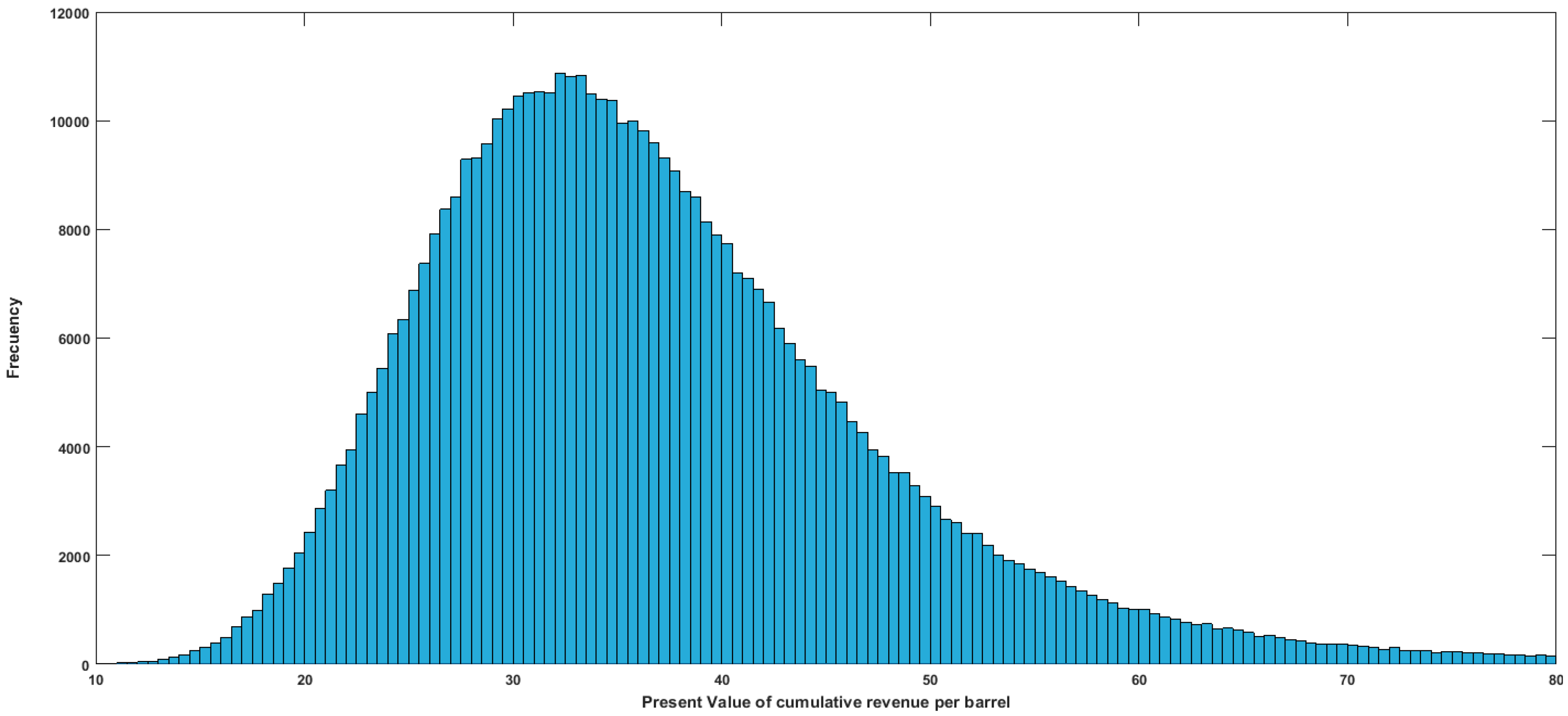
The results are displayed in Figure 6; they draw on the parameter estimates in Table 2. The average of our MC simulations is $37.18/bbl; this figure differs only slightly (0.3%) from the analytical value $i(S_0,S_0^{*},10)=37.07$ that resulted from Equation (17).

Now, the so-called VaR addresses the question of how much a company could deviate from its average or expected performance (on the downside) with a given confidence level. In our case, the VaR(95%) is $22.22/bbl. This means that $i(S_0,S_0^{*},10)$ will fall below 22.22 in the worst 5% of the cases.

The distribution in Figure 6 is far from symmetric (unlike a Gaussian distribution). Besides, fat tails or other deviations from normality cannot be discarded. For this reason, in addition to the above standard measure of risk we compute the so-called ES, or ES(95%), which is more sensitive to the shape of the loss tail. It measures the average value of $i(S_0,S_0^{*},10)$ in the 5% of worst cases: $19.77/bbl. This value is close to the cost of producing oil in the best Saudi Arabian fields. In the case of U.S. tight-oil producers, costs are higher, so their NPV will certainly be negative more than 5% of the cases.

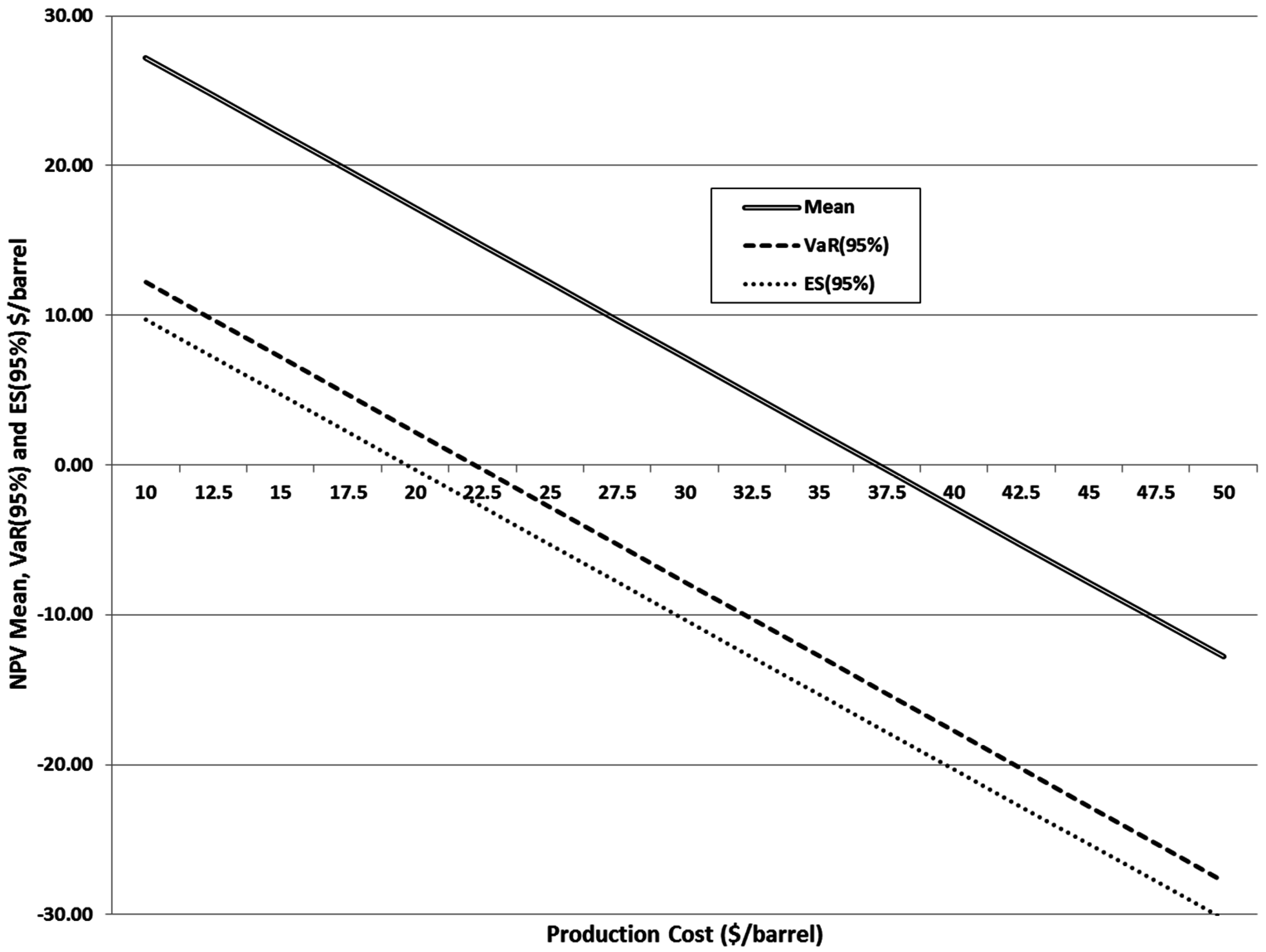
Figure 7 below shows the average NPV (per barrel of reserves), NPV, along with the VaR and the ES as a function of the (unit) production cost of tight oil, c. Equation (19) above shows a linear, negative relationship between the NPV and c; therefore, the NPV is represented by a downward-sloping straight line in this space. The same holds for VaR(95%) and ES(95%). The NPV is positive whenever the cost is lower than $37.18/bbl. Looking beyond central moments, the 5% worst-case scenarios start at a cost of $22.22/bbl. In other words, if the oil field’s cumulative income falls to the VaR(95%) level then a cost of $22.22/bbl implies NPV = 0. Within this region the average revenue is $19.77/bbl, so a unit cost above 19.77 pushes the average NPV into negative territory.

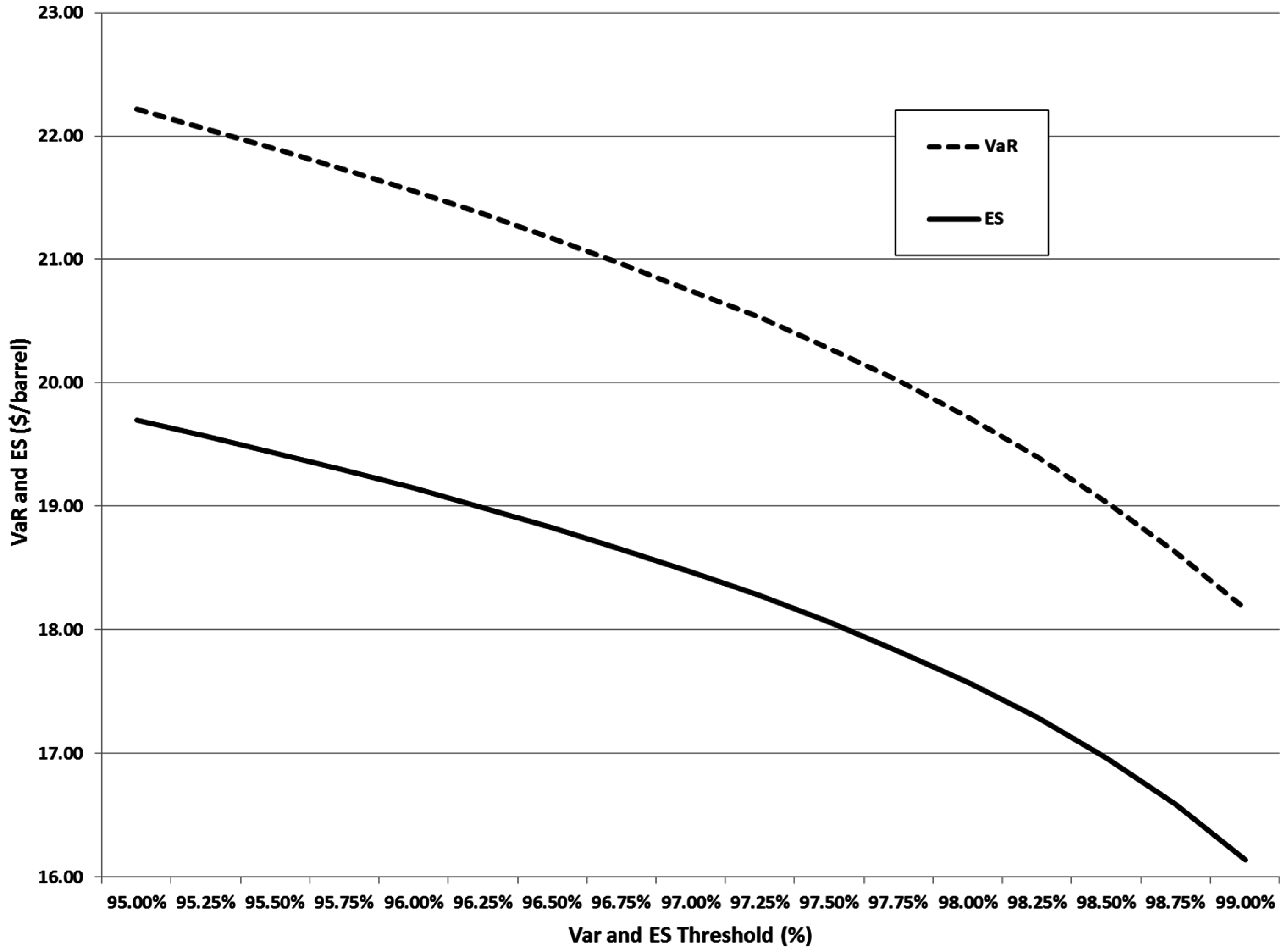
On the other hand, up to now we have adopted the standard worst-case threshold level for both the VaR and the ES, namely 5%. Nonetheless, we can be interested in the impact of even more stringent scenarios on oil producers’ revenues. Figure 8 displays how our earlier thresholds ($22.22/bbl and 19.77, respectively) change as we look at ever worse scenarios. Not surprisingly, the PV of the cumulative cash inflow along the left tail of the distribution decreases. The most extreme scenario considered (1%) entails a drop in the VaR and ES of cumulative revenue around 20% relative to the traditional thresholds.

7. Sensitivity Analysis

The above numerical results are obviously contingent on the particular sample period considered (from 24 February 2006 to 4 February 2016). In the final part of this period the oil price was abnormally subdued, at some points swinging around $30 a barrel. Our estimates of S₀ and $S_0^{*}$ ($31.36/bbl and $49.94/bbl, respectively) emerge from these futures prices. Below we perform some sensitivity analyses with respect to changes in the spot price and the long-term price. As before, we are interested in the impact on the risk profile of cumulative revenues and the two measures or risk.

We consider four potential values of S₀ (namely $20, $30, $40, and $50 per barrel) and combine them with three values of $S_0^{*}$ ($40, $50, and $60 per barrel). The latter values can be seen as conservative when compared with other sources. For example [13], analyzes two different scenarios in which oil prices rise back to either $70/bbl or $90/bbl. Note, though, that we are focusing on the risks faced by current tight-oil producers. Our prices are not meant to be required for luring capital back in or incentivizing new, long-term investments at the global level. Our price levels are more in line with one of the forecasts in [12], where crude prices are assumed to rebound to $60–$65 a barrel for an extended period and rigs continue in operation (or drillers put them back to work).

Table 4. Sensitivity Analysis.

S0	${\mathit{S}}_0^{*}$	Average $\mathit{i}({\mathit{S}}_0,{\mathit{S}}_0^{*},10)$	VaR(95%)	ES(95%)
20.00	40.00	26.51	16.02	14.27
20.00	50.00	29.93	18.26	16.28
20.00	60.00	33.36	20.48	18.27
30.00	40.00	32.91	19.49	17.31
30.00	50.00	36.34	21.77	19.37
30.00	60.00	39.76	24.04	21.41
40.00	40.00	39.32	22.89	20.27
40.00	50.00	42.75	25.22	22.38
40.00	60.00	46.17	27.50	24.46
50.00	40.00	45.73	26.26	23.20
50.00	50.00	49.15	28.61	25.34
50.00	60.00	52.58	30.94	27.45

shows the results. The reference case (S₀ = $31.36/bbl, and $S_0^{*}$ = $49.94/bbl) is well represented by the central line in the second block (S₀ = $30/bbl, and $S_0^{*}$ = $50/bbl). Now, let us set the long-term price at $50/bbl while changing the initial spot price from $40/bbl to $50/bbl (a 25% increase). In this case, the PV of the cumulative revenue jumps from $42.75/bbl to $49.15/bbl, an increase of 15%. Our two measures of risk increase too, although at a slightly lower rate (around 13%). Therefore, the unit cost required for turning the NPV to negative rises significantly and the prospects for oil producers improve accordingly. We can adopt another perspective on this issue. Specifically, now we fix S₀ at $50/bbl and change $S_0^{*}$ from $40/bbl to $50/bbl (again a 25% increase). In this case, $i(S_0,S_0^{*},10)$^* grows by 7.5% (from $45.73/bbl to $49.15/bbl) and our variables of interest grow around 9%. As in Section 5, $i(S_0,S_0^{*},10)$ is relatively more affected by changes in the spot price than the future price; this is consistent with intense depletion at the beginning followed by a steep decline thereafter.

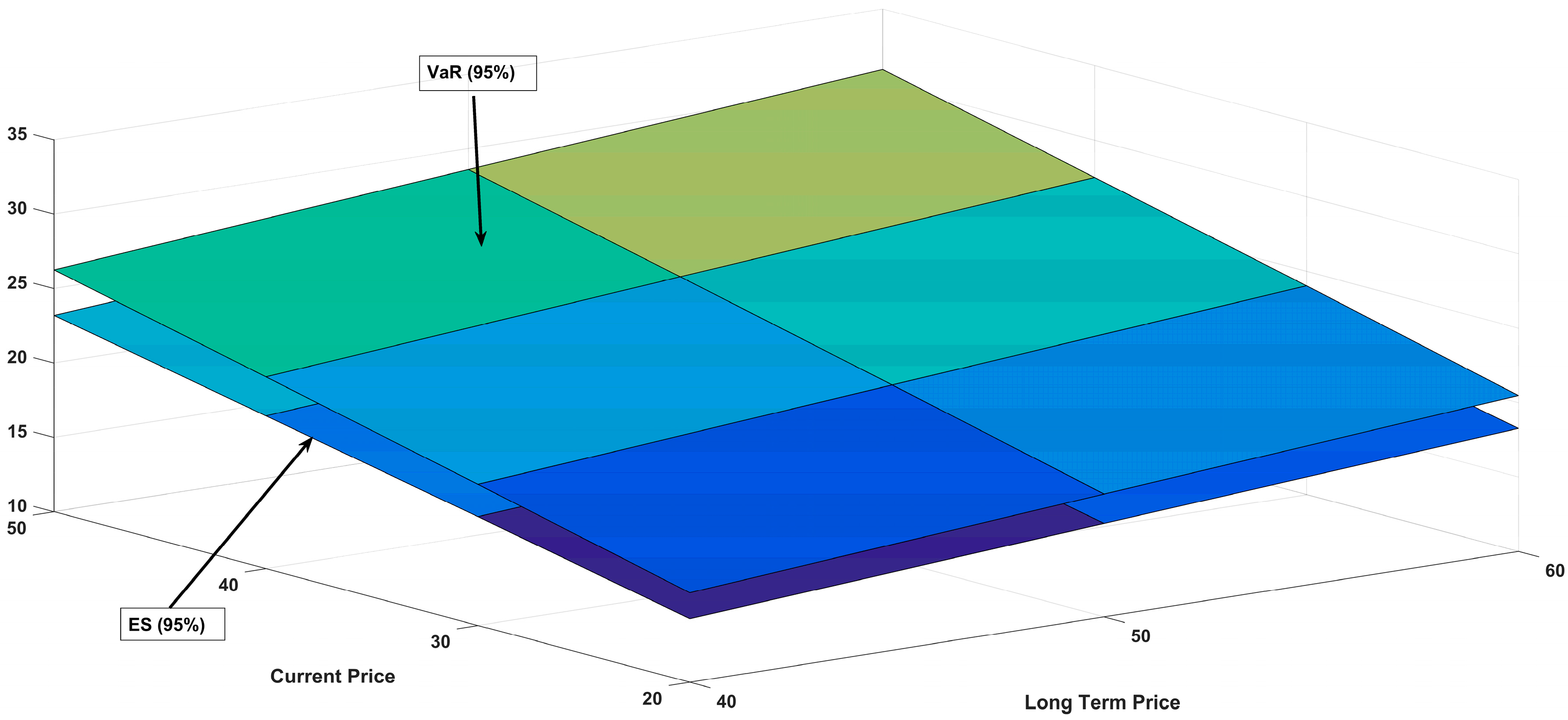
The particular changes in our measures of risk are displayed in Figure 9. The starting level of the 5% left tail, VaR(95%), is naturally higher than the average value over that tail, ES(95%), so the former always evolves above the latter. This said, their respective behaviors are pretty much parallel. For a given level of one price, a higher level of the other price entails an increase in both statistical measures (and, consequently, a higher unit cost required to turn operations uneconomic). At the same time, the sensitivity of these measures to both prices is more or less balanced.

8. Conclusions

This paper addresses the prospects for U.S. producers of tight oil with a special focus on their revenues. The behavior of the oil price in the future is paramount since it determines whether production is profitable or not. We introduce a stochastic model for the spot price of oil that allows for mean reversion. The long-run level toward which the spot price tends to revert is itself stochastic. And the volatility of price changes is similarly assumed to be stochastic and mean reverting. These three processes can well be correlated. Hence we develop a model for the (gross) value of an operating tight-oil field. Specifically we compute the PV of the revenues to be collected over the production/valuation horizon; for convenience we measure it in unit terms (i.e., per barrel of reserves). This PV of cumulative revenues can be set against the PV of the costs (per barrel of reserves) to be faced in the future. Producers would make a profit or a loss depending on whether the resulting NPV is positive or not.

We estimate the model with daily prices of the ICE WTI Light Sweet Crude Oil Futures Contract traded on the ICE. The sample period goes from February 2006 to February 2016. According to our results, the PV of the prospective revenues up to ten years from now amounts to $37.07/bbl in the base case. Thus, production from an operating tight-oil field will make sense provided the cost of producing a barrel of oil is lower than $37.07. Needless to say, any numerical estimate must be taken as (more or less) accurate on average at best, if only because the tight-oil sector is rather heterogeneous.

This threshold is contingent on the initial spot price of oil and the initial estimate of the long-term price (which were both relatively low even by current standards). Not surprisingly, if both prices increase, the PV of the cumulative cash inflow will increase too. Yet their relative importance is far from symmetric; in particular, the former has a stronger impact. Anyway the bottom line is that the paper shows how the extraction decision draws on spot and futures prices.

In addition, we ran a MC simulation to get a deeper knowledge of the underlying risks and check the robustness of our results. The VaR measures how much a company could deviate from its average or expected performance (on the downside) with a given confidence level. In our case, the VaR(95%) is $22.22/bbl. This means that the PV of the cumulative revenue (per barrel) will fall below $22.22 in the worst 5% of the cases. We also compute the so-called ES, or ES(95%), which is more sensitive to the shape of the loss tail. It measures the average value of the former PV in the 5% of worst scenarios; in our case it is $19.77/bbl. Further, when the worst-case threshold is reduced from 5% to 1% both the VaR and the ES of cumulative revenue decrease by around 20% relative to the earlier levels. Overall, the paper shows how to compute the risks underlying the decision to operate a tight-oil field. This decision must be re-evaluated continuously as new information arrives and uncertainty about the future unfolds. For example, it can be rational to interrupt the operation of a previously profitable field if an abrupt, unexpected fall in oil prices renders it unprofitable.

As already mentioned, our above numerical results are contingent on our particular sample period. This is why we have also performed some sensitivity analyses with respect to changes in the spot price and the long-term price. Thus, for example, we fix the long-run oil price at $50/bbl while changing the initial spot price from $40 to $50 per barrel (a 25% increase). In this case, the PV of the cumulative revenue increases by 15%, and our two measures of risk increase around 13%. Alternatively, we can fix the initial spot price at $50/bbl and change the long-run price from $40 to $50 per barrel (again a 25% increase). In this case, the PV of the cumulative revenue grows by 7.5% while our two measures of risk grow around 9%. This stronger reaction to immediate events bodes will with the time profile of production of tight oil: intense depletion initially, followed by steep decline thereafter.

At this point some qualifications are in order. Oil prices in particular can be anticipated to remain low for a while [12]. Storage tanks in the U.S. are at their fullest since 1930. The fracklog, i.e., the number of wells waiting to be hydraulically fractured, has grown threefold: firms naturally aim to avoid oil extraction when the oil price is low, and defer completion work accordingly. The fracklog may slow a recovery in oil prices, as companies opt to bring back shale where the lead times are short and oil production can be quickly ramped-up to maximum levels.

In our analysis production costs are assumed deterministic and exogenously given. In particular they are independent of oil price. But if oil prices eventually increase, maybe costs will follow suit (cost cycling).

We have made no mention of taxes. However, governments extract money from oil companies through a range of levies, royalties, severance taxes, production sharing agreements, etc.; see for instance [33]. As a matter of fact, most shale resources do not lie beneath federal land. Reference [9] estimates that federal royalties from these resources will total about $300 M a year by 2024. Therefore, states (and lower-level authorities) have a great say on the prospects for shale producers, e.g., via oil severance taxes, but also through tax incentives (such as credits or lower rates) when oil prices are low. Nonetheless, federal authorities can still affect shale development in a number of ways, e.g., through oil export policies, climate and environmental regulation, infrastructure development programs, etc.

We have left aside the decision whether to complete a DUC or not (exploration costs are already sunk). This is clearly a real option that oil managers have at their disposal. Some other options (similarly beyond the scope of this paper) refer to the possibility of temporarily closing in an active well, or abandoning it completely, drilling a new well, and so on. Paying attention to option-like issues is precisely one of the major approaches to raising the productivity of capital in this extremely capital-intensive industry; see [6].

Last, as [34] points out, the terms of oil and gas leases have both individual and collective significance since they specify a range of practices which can influence social, economic and/or environmental outcomes of development. In our case, the pairing of horizontal drilling and hydraulic fracturing comes with a broader suit of spatial impacts [35]. These impacts should ultimately be considered alongside regional and global benefits.

References

- Data Set: U.S. Crude Oil Production, 1990–2035; U.S. Energy Information Administration (US EIA): Washington, DC, USA, 2012.
- Energy in Brief: Shale in the United States; U.S. Energy Information Administration (US EIA): Washington, DC, USA, 2016.
- Glossary of Energy and Financial Terms; Chevron Corporation: San Ramon, CA, USA, 2015.
- Medium-Term Oil and Gas Markets 2011; International Energy Agency (IEA): Paris, France, 2011.
- Drilling Sideways: A Review of Horizontal Well Technology and Its Domestic Application; DOE/EIA-TR-0565; U.S. Energy Information Administration (US EIA): Washington, DC, USA, 1993.
- Xu, S. RBL: Redeterminations Different in 2016. Oil & Gas Financial Journal, Tulsa, OK, USA, 16 May 2016. [Google Scholar]
- Shale Wells are Getting More Profitable Every Year; Rystad Energy: Oslo, Norway, 2016.
- Editorial: Oil Price Review. Oil Energy Trends 2016, 41, 10–12.
- The Economic and Budgetary Effects of Producing Oil and Natural Gas from Shale; U.S. Congressional Budget Office: Washington, DC, USA, 2014.
- Baumeister, C.; Kilian, L. Forty years of oil price fluctuations: Why the price of oil may still surprise us. J. Econ. Perspect. 2016, 30, 139–160. [Google Scholar] [CrossRef]
- The Economist. Fracking Companies. DUC and Cover. 12 March 2016. Available online: http://www.economist.com/news/business/21694522-rising-oil-prices-will-not-quickly-rescue-beleaguered-shale-industry-duc-and-cover (accessed on 3 May 2016).
- Doan, L.; Murtaugh, D. U.S. Shale Fracklog Triples as Drillers Keep Oil from Market. Bloomberg. 23 April 2015. Available online: http://www.bloomberg.com/news/articles/2015-04-23/u-s-shale-fracklog-triples-as-drillers-keep-oil-out-of-market-i8u004xl (accessed on 22 February 2016).
- Annex, M. White Paper: Is the US Chemical Renaissance a Flash in the Pan? Bloomberg New Energy Finance. 20 January 2014. Available online: http://www.ourenergypolicy.org/white-paper-is-the-us-chemicals-renaissance-a-flash-in-the-pan/ (accessed on 16 October 2015).
- Brealey, R.; Myers, S.C.; Allen, F. Principles of Corporate Finance, 10th ed.; McGraw-Hill: New York, NY, USA, 2010. [Google Scholar]
- Bloomberg Intelligence. Break-Even Model: Cracking the Shale Enigma. 8 February 2016. Available online: https://www.bloomberg.com/professional/blog/break-even-model-cracking-the-shale-enigma/ (accessed on 2 June 2015).
- Upstream Oil & Gas Asset Based Model—CDR; Rystad Energy: Oslo, Norway, 2014.
- Bloomberg Intelligence. When Will the “Call” on U.S. Oil Supply Return? 14 April 2016. Available online: https://www.bloomberg.com/professional/blog/when-will-the-call-on-u-s-oil-supply-return/ (accessed on 14 September 2016).
- Lower for Longer. Oil & Gas Financial Journal, Tulsa, OK, USA, 15 May 2016.
- Brennan, M.; Schwartz, E. Evaluating natural resource investments. J. Bus. 1985, 58, 135–157. [Google Scholar] [CrossRef]
- McDonald, R.L.; Siegel, D.R. Investment and the valuation of firms when there is an option to shut down. Int. Econ. Rev. 1985, 26, 331–349. [Google Scholar] [CrossRef]
- Bjersund, P.; Ekern, S. Contingent Claims Evaluation of Mean-Reverting Cash Flows in Shipping. In Real Options in Capital Investment: Models, Strategies, and Applications; Trigeorgis, L., Ed.; Praeger: Westport, CT, USA, 1993. [Google Scholar]
- Schwartz, E.S. The stochastic behavior of commodity prices: Implications for valuation and hedging. J. Financ. 1997, 52, 923–973. [Google Scholar] [CrossRef]
- Pilipovic, D. Energy Risk; McGraw-Hill: New York, NY, USA, 1998. [Google Scholar]
- Pilipovic, D. Energy Risk: Valuing and Managing Energy Derivatives, 2nd ed.; McGraw-Hill: New York, NY, USA, 2007. [Google Scholar]
- Abadie, L.M.; Chamorro, J.M. Valuing expansions of the electricity transmission network under uncertainty: The binodal case. Energies 2011, 4, 1696–1727. [Google Scholar] [CrossRef]
- Abadie, L.M.; Galarraga, I.; Rübbelke, D. Evaluation of two alternative carbon capture and storage technologies: A stochastic model. Environ. Model. Softw. 2014, 54, 182–195. [Google Scholar] [CrossRef]
- Bhattacharya, S. Project valuation with mean reverting cash flow streams. J. Financ. 1978, 33, 1317–1331. [Google Scholar] [CrossRef]
- Brennan, M.; Schwartz, E. Analyzing convertible bonds. J. Financ. Quant. Anal. 1980, 15, 907–929. [Google Scholar] [CrossRef]
- Insley, M.A. Real options approach to the valuation of a forestry investment. J. Environ. Econ. Manag. 2002, 44, 471–492. [Google Scholar] [CrossRef]
- Abadie, L.M.; Chamorro, J.M. Valuation of wind energy projects: A real options approach. Energies 2014, 7, 3218–3255. [Google Scholar] [CrossRef]
- Lewis, A. Option Valuation under Stochastic Volatility: With Mathematica Code; Finance Press: Newport Beach, CA, USA, 2000. [Google Scholar]
- Abadie, L.M.; Chamorro, J.M. Investments in Energy Assets under Uncertainty; Springer: London, UK, 2013. [Google Scholar]
- Taxation and Oil Companies. Oiling the Wheels. The Economist. 19 March 2016. Available online: http://www.economist.com/news/business/21695016-governments-are-easing-tax-burden-industry-some-exceptions-oiling-wheels (accessed on 12 May 2016).
- Bugden, D.; Kay, D.; Glynn, R.; Stedman, R. The bundle below: Understanding unconventional oil and gas development through analysis of lease agreements. Energy Policy 2016, 92, 214–219. [Google Scholar] [CrossRef]
- Mauter, M.S.; Palmer, V.R.; Tang, Y.; Behrer, A.P. The Next Frontier in United States Shale Gas and Tight Oil Extraction: Strategic Reduction of Environmental Impacts; Energy Technology Innovation Policy Research Group; Belfer Center for Science and International Affairs, Harvard Kennedy School: Cambridge, MA, USA, 2013. [Google Scholar]
Figure 1.
Monthly production and rig count in the key tight-oil U.S. regions. Source: Energy Information Administration (EIA).
Figure 2.
West Texas Intermediate (WTI) spot and longest-maturity futures prices. Source: EIA and Intercontinental Exchange (ICE), respectively.
Figure 3.
ICE WTI futures price curve (4 February 2016, the last sample day). Source: ICE.
Figure 4.
Return volatility as a function of the contract maturity over the sample period.
Figure 5.
WTI crude oil price volatility (25-day moving window).
Figure 6.
Probability distribution of the PV of income from tight oil ($/bbl).
Figure 7.
Unit net present value (NPV) (average), value at risk (VaR), and expected shortfall (ES) as a function of unit production costs.
Figure 8.
Revenue VaR and ES as a function of the probability cut-off threshold.
Figure 9.
Sensitivity of VaR(95%) and ES(95%) to the spot price (S0) and future price ().