
Solar Resource for Urban Communities in the Baja California Peninsula, Mexico


Abstract
:
1. Introduction
2. Materials and Methods
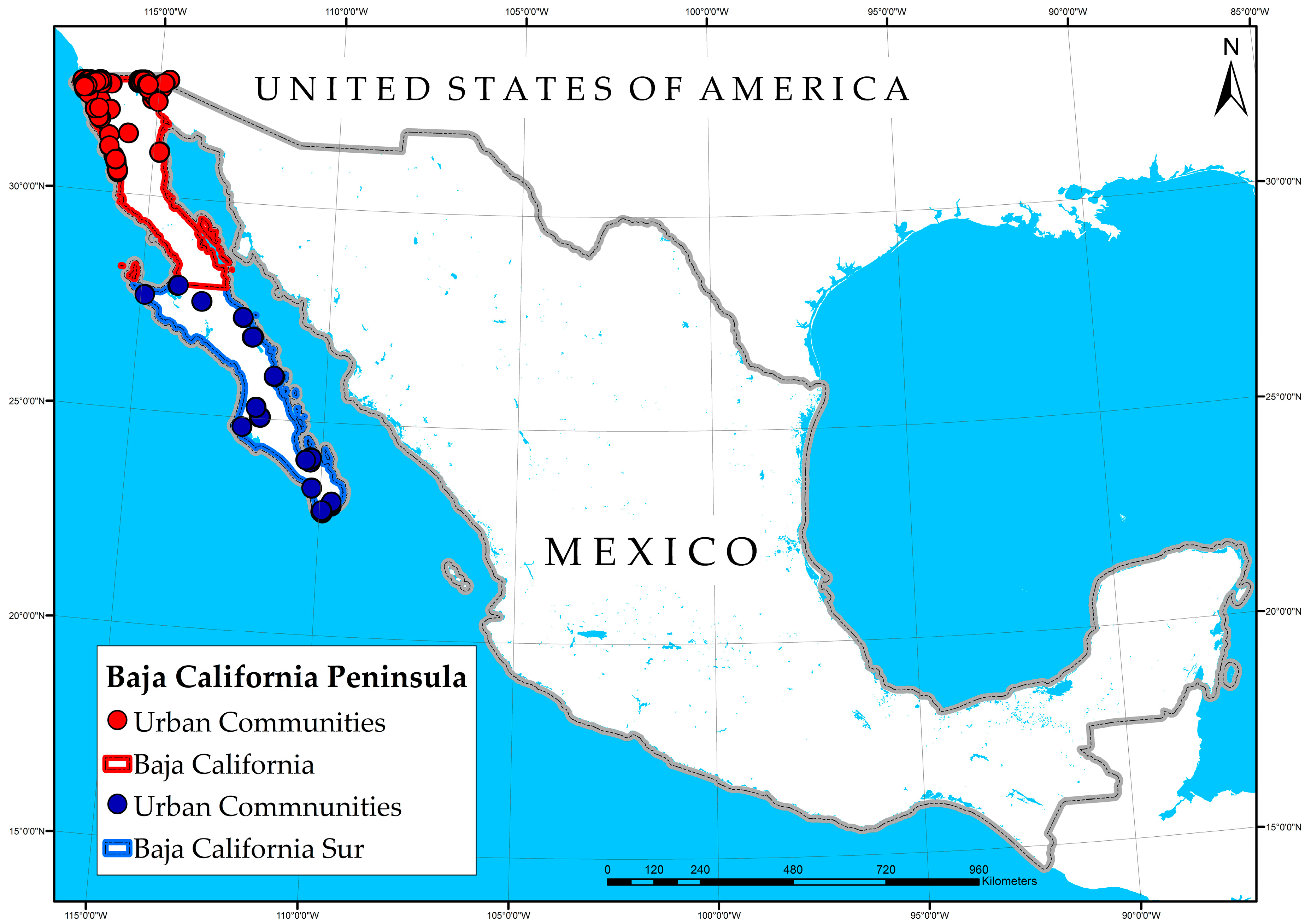
2.1. Ground Data
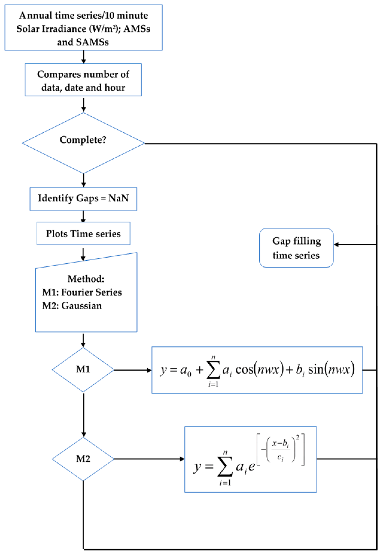
2.2. Methods
2.3. Typical Meterological Year
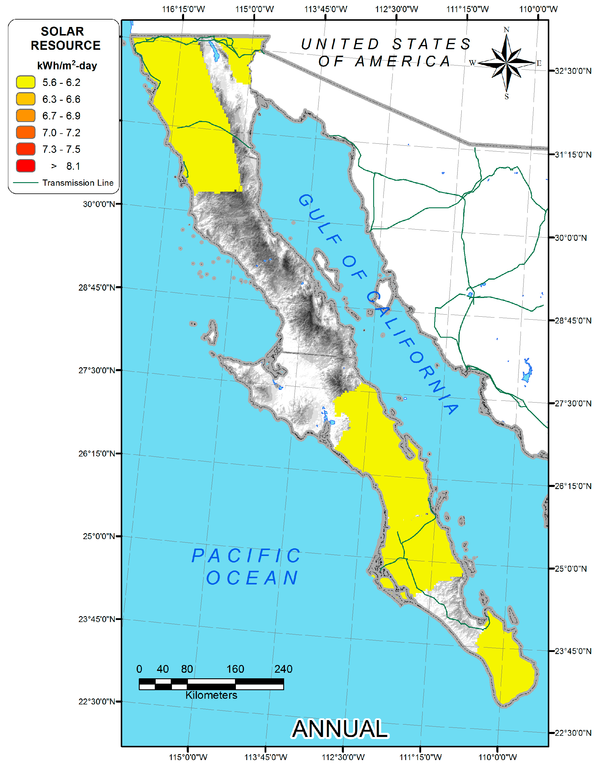
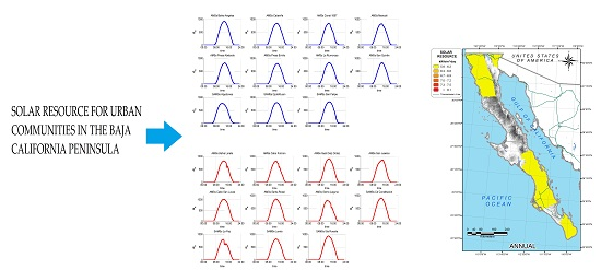
2.4. Solar Resource Maps in the Baja California Peninsula
3. Results
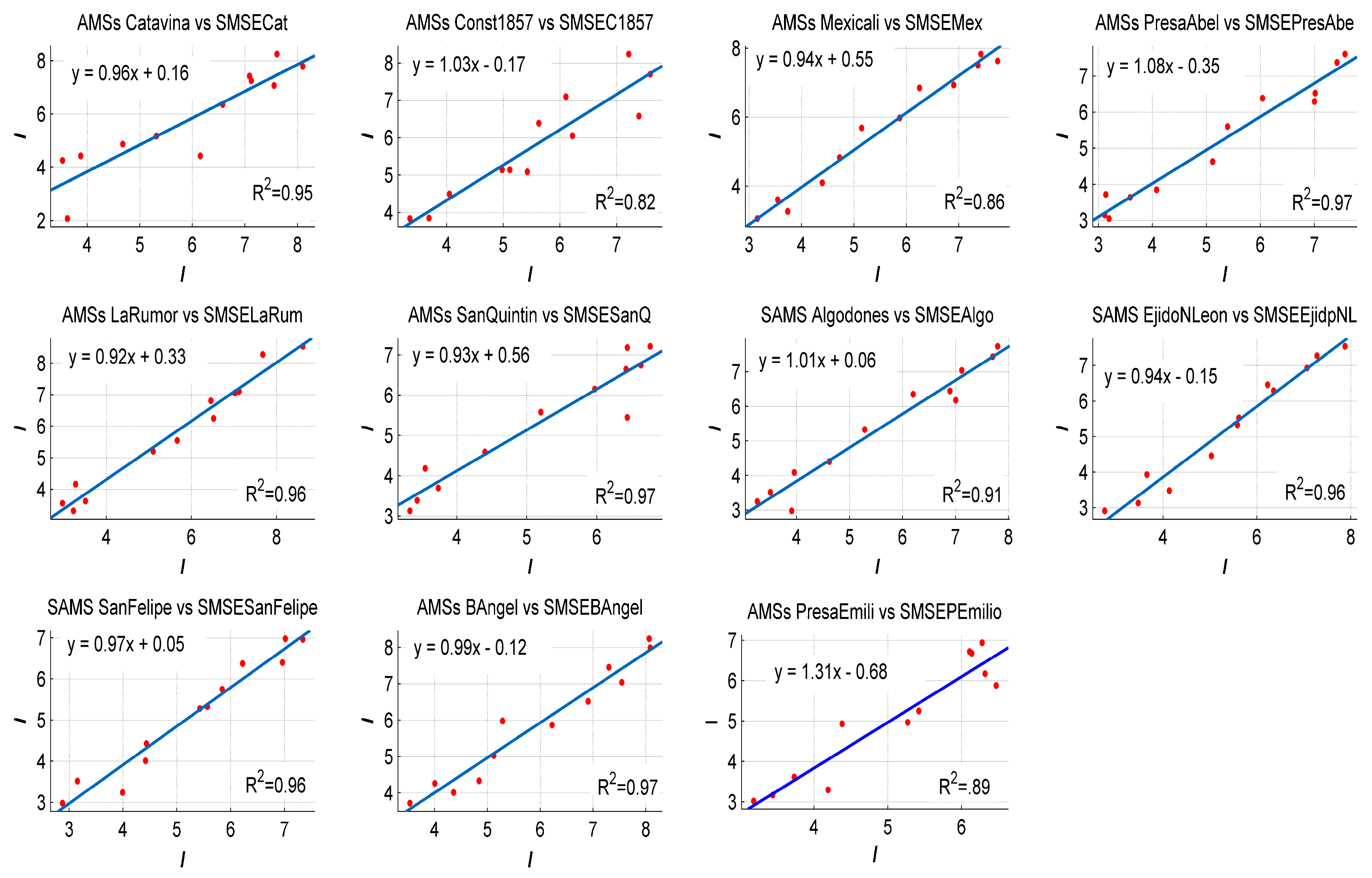
3.1. Validation
3.2. Solar Resource
3.2.1. Daily Pattern
3.2.2. Solar Irradiation
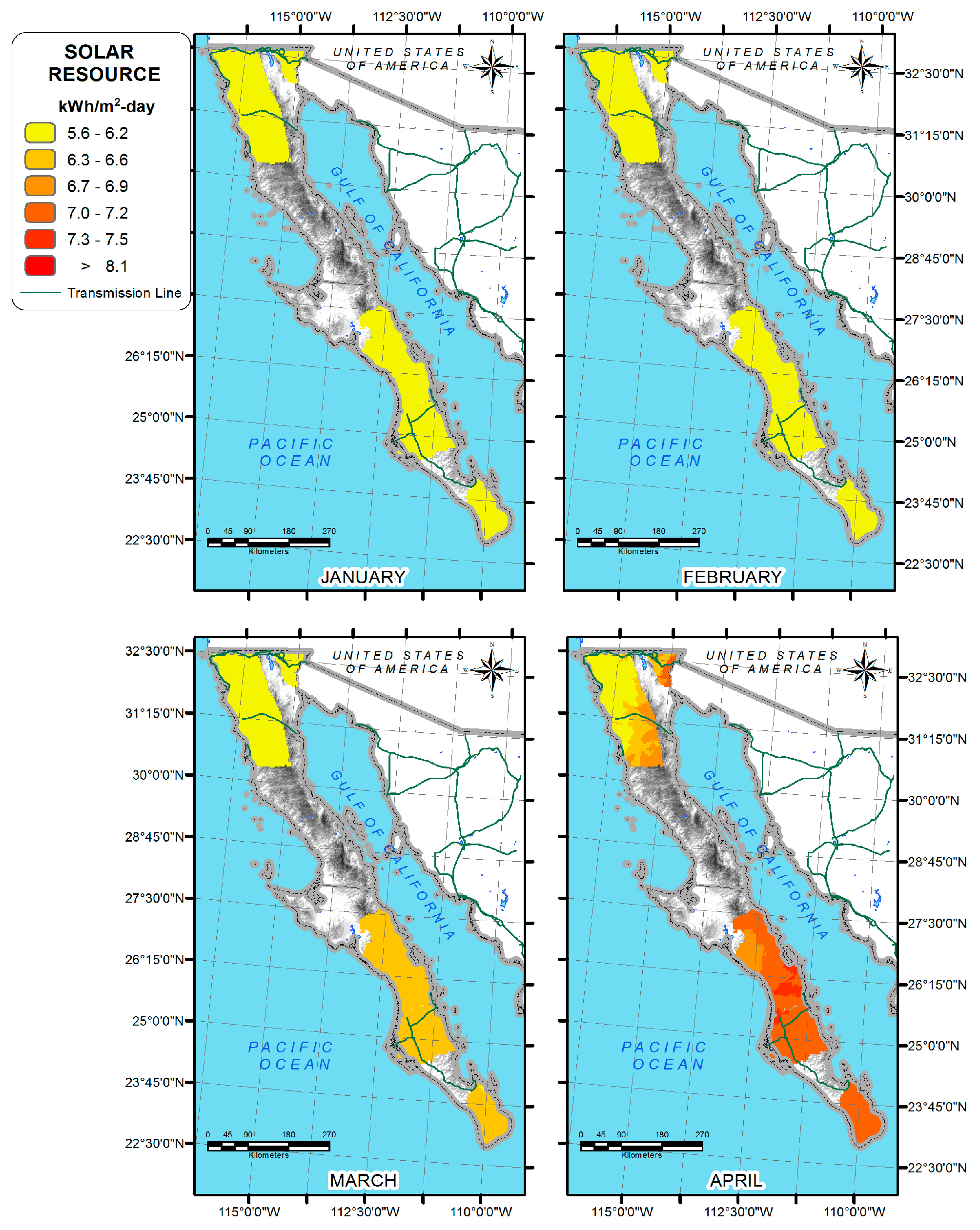
3.2.3. Solar Maps
4. Discussion
5. Conclusions
Acknowledgments
Author Contributions
Conflicts of Interest
Abbreviations
| AMS | Automatic Meteorological Stations |
| SAMS | Synoptic Automatic Meteorological Station |
| NMS | National Meteorological System of Mexico |
| SMSE | Surface and Meteorology Energy System |
| GIS | Geographic Information System |
| GWh | Gigawatts-hour |
| MW | Megawatt |
| PV | Photovoltaic |
| CSP | Concentrated Solar Power |
| MWh | Megawatt-hour |
| RMSE | Root Mean Square Error |
| SSE | Error Sum of Squares |
| SSR | Regresion Sum of Squares |
| SST | Total Sum of Squares |
| TMY | Typical Meteorological Year |
References
- International Energy Agency (IEA). Available online: http://energyatlas.iea.org (accessed on 4 February 2016).
- Castellano, N.N.; Gázquez Parra, J.A.; Valls-Guirado, J.; Manzano-Agugliaro, F. Optimal displacement of photovoltaic array’s rows using a novel shading model. Appl. Energy 2015, 144, 1–9. [Google Scholar] [CrossRef]
- Hasanuzzaman, M.; Malek, A.B.M.A.; Islam, M.M.; Pandey, A.K.; Rahim, N.A. Global advancement of cooling technologies for PV systems: A review. Sol. Energy 2016, 137, 25–45. [Google Scholar] [CrossRef]
- De la Tour, A.; Glachant, M.; Meniere, Y. Innovation and international technology transfer: The case of the Chinese photovoltaic industry. Energy Policy 2011, 39, 761–770. [Google Scholar] [CrossRef] [Green Version]
- The International Renewable Energy Agency (IRENA). Renewable Power Generation Costs. Available online: http://www.IRENA.org/DocumentDownloads/Publications/IRENA_RE_Power_Costs_2014_report.pdf (accessed on 30 September 2016).
- Bloomberg. The Way Humans Get Electricity Is About to Change Forever, Bloomberg Business. Available online: http://www.bloomberg.com/news/articles/2015-06-23/the-way-humans-get-electricity-is-about-to-change-forever (accessed on 30 September 2016).
- Ondraczek, J.; Komendantova, N.; Patt, A. WACC the dog: The effect of financing costs on the levelized cost of solar PV power. Renew. Energy 2015, 75, 888–898. [Google Scholar] [CrossRef]
- Ryan, L.; Dillon, J.; Monaca, S.L.; Byrne, J.; O’Malley, M. Assessing the system and investor value of utility-scale solar PV. Renew. Sustain. Energy Rev. 2016, 64, 506–517. [Google Scholar] [CrossRef]
- Zhu, H.; Li, X.; Sun, Q.; Nie, L.; Yao, J.; Zhao, G. A power prediction method for photovoltaic power plant based on wavelet decomposition and artificial neural networks. Energies 2016, 9, 11. [Google Scholar] [CrossRef]
- Secretaria de Energia (SENER). Available online: http://sie.energia.gob.mx (accessed on 4 February 2016).
- Comision Nacional para el Uso Eficiente de la Energia (Conuee). Available online: http://www.conuee.gob.mx (accessed on 20 May 2016).
- Hernandez-Escobedo, Q.; Rodriguez-Garcia, E.; Saldana-Flores, R.; Garcia-Fernandez, A. Manzano-Agugliaro, F. Solar energy resource assessment in the Mexican states along the Gulf of Mexico. Renew Sust. Energy Reviews. 2015, 43, 216–238. [Google Scholar] [CrossRef]
- Sosa-Tinoco, I.; Peralta-Jaramillo, J.; Otero-Casal, C.; Lopez-Aguera, A.; Miguez-Machi, G.; Rodriguez-Cabo, I. Validation of a global horizontal irradiation assessment from a numerical weather prediction model in south of Sonora-Mexico. Renew. Energy 2016, 90, 105–113. [Google Scholar] [CrossRef]
- The World Bank. Available online: http://data.worldbank.org/indicator/SI.POV.RUHC (accessed on 5 February 2016).
- Comision Federal de Electricidad (CFE). Available online: http://cfe.gob.mx (accessed on 5 February 2016).
- Instituto Nacional de Estadistica y Geografia (INEGI). Available online: www.inegi.org.mx (accessed on 5 February 2016).
- Energetic Information System, Mexico. Available online: http://cfe.gob.mx (accessed on 4 April 2016).
- Energetic Transition Law (ETL). Available online: http://dof.gob.mx (accessed on 7 February 2016).
- National Meteorological Service Mexico (NMS). Available online: http://smn.gob.mx (accessed on 4 January 2016).
- Surface Meteorology and Solar Energy (SMSE). Available online: https://eosweb.larc.nasa.gov/sse/ (accessed on 7 January 2016).
- Polo, J.; Zarzalejo, L.F.; Cony, M.; Navarro, A.A.; Marchante, R.; Martin, L. Solar radiation estimations over India using Meteosat satellite images. Sol. Energy 2011, 85, 2395–2406. [Google Scholar] [CrossRef]
- Zelenka, A.; Perez, R.; Seals, R.; Renne, D. Effective accuracy of satellite-derived hourly irradiations. Theor. Appl. Climatol. 1999, 62, 199–207. [Google Scholar] [CrossRef]
- Vignola, F.; Harlan, P.; Perez, R.; Kmiecik, M. Analysis of satellite derived beam and global solar radiation data. Sol. Energy 2007, 81, 768–772. [Google Scholar] [CrossRef]
- Pedro, H.T.C.; Coimbra, C.F.M. Assessment of forecasting techniques for solar power production with no exogenous inputs. Sol. Energy 2012, 86, 2017–2028. [Google Scholar] [CrossRef]
- Lee, K.; Yoo, H.; Levermore, G. Quality control and estimation hourly solar irradiation on inclined surfaces in South Korea. Renew. Energy 2013, 57, 190–199. [Google Scholar] [CrossRef]
- Maghrabi, A.H. Parameterization of a simple model to estimate monthly global solar radiation based on meteorological variables, and evaluation of existing solar radiation models for Tabouk, Saudi Arabia. Energy Convers. Manag. 2009, 50, 1754–2760. [Google Scholar] [CrossRef]
- Wu, G.; Liu, Y.; Wang, T. Methods and strategy for modeling daily global solar radiation with measured meteorological data—A case study in Nanchang station, China. Energy Convers. Manag. 2007, 48, 2447–2452. [Google Scholar] [CrossRef]
- User’s Manual for TMY2s Typical Meteorological Years. Available online: http://rredc.nrel.gov/solar/pubs/tmy2/pdfs/tmy2man.pdf (accessed on 1 November 2016).


| Source | Meteorological Station | State | N (°) | W (°) | Altitude |
|---|---|---|---|---|---|
| AMS | Bahia Angeles | Baja California | 28.8964 | 113.5603 | 10 |
| AMS | Catavina | Baja California | 29.7272 | 114.7192 | 514 |
| AMS | Const. 1857 | Baja California | 32.0419 | 115.9217 | 1576 |
| AMS | Mexicali | Baja California | 32.6669 | 115.2908 | 50 |
| AMS | Presa Abelardo L. | Baja California | 32.4472 | 116.9083 | 156 |
| AMS | Presa Emilio Lo | Baja California | 31.8913 | 116.6033 | 32 |
| AMS | La Rumorosa | Baja California | 32.2722 | 116.2056 | 1262 |
| AMS | San Quintin | Baja California | 30.5317 | 115.8375 | 32 |
| SAMS | Algodones | Baja California | 32.7047 | 114.7303 | 40 |
| SAMS | Ejido Nvo. Leon | Baja California | 32.4128 | 115.1919 | 11.4 |
| SAMS | San Felipe | Baja California | 31.0281 | 114.8344 | 20 |
| AMS | Bahia de Loreto | Baja California Sur | 26.0097 | 111.3539 | 1 |
| AMS | Cabo Pulmon | Baja California Sur | 23.4450 | 109.4244 | 25.9 |
| AMS | Gust Diaz Ordaz | Baja California Sur | 27.6428 | 113.4575 | 37 |
| AMS | San Juanico | Baja California Sur | 26.2575 | 112.4786 | 36 |
| AMS | Cabo San Lucas | Baja California Sur | 22.8811 | 109.9267 | 224 |
| AMS | Santa Rosalia | Baja California Sur | 27.3381 | 112.2694 | 53 |
| AMS | Sierra Laguna | Baja California Sur | 23.5553 | 109.9986 | 1949 |
| SAMS | Cd Constitucion | Baja California Sur | 25.0097 | 111.6467 | 48 |
| SAMS | La Paz | Baja California Sur | 24.1167 | 110.3167 | 18 |
| SAMS | Loreto | Baja California Sur | 26.0114 | 111.3500 | 15 |
| SAMS | Sta Rosalia | Baja California Sur | 27.2833 | 112.2500 | 82 |
| Source | SSE | R-Square | RMSE | MAE | Bias | |
|---|---|---|---|---|---|---|
| kWh/m2/day | ||||||
| Bahia Angeles | SMSE_Ban | 1.45149 | 0.95 | 0.38098 | 0.16 | 0.032 |
| Catavina | SMSE_Cat | 6.89759 | 0.82 | 0.83052 | 0.29 | 0.150 |
| Const. 1857 | SMSE_C1857 | 3.17617 | 0.86 | 0.56358 | 0.23 | 0.082 |
| Mexicali | SMSE_Mex | 0.92855 | 0.97 | 0.30472 | 0.14 | 0.037 |
| Presa Abelardo L | SMSE_PrAbe | 1.31309 | 0.96 | 0.36237 | 0.12 | 0.025 |
| Presa Emilio Lo | SMSE_PEmilio | 2.50370 | 0.89 | 0.50040 | 0.14 | 0.032 |
| La Rumorosa | SMSE_Rum | 1.08316 | 0.97 | 0.32911 | 0.21 | 0.058 |
| San Quintin | SMES_SanQuin | 2.21336 | 0.91 | 0.47046 | 0.17 | 0.051 |
| Algodones | SMSE_Algod | 1.36899 | 0.96 | 0.37000 | 0.27 | 0.089 |
| Ejido Nvo. Leon | SMSE_Ejido | 0.96154 | 0.97 | 0.31009 | 0.16 | 0.052 |
| San Felipe | SMSE_SanFelipe | 1.02661 | 0.96 | 0.32041 | 0.23 | 0.063 |
| Bahia de Loreto | SMSE_BLoreto | 1.67932 | 0.92 | 0.40980 | 0.15 | 0.032 |
| Cabo Pulmon | SMSE_CabP | 2.44898 | 0.84 | 0.49487 | 0.24 | 0.073 |
| Gust Diaz Ordaz | SMSE_Gdiaz | 1.04616 | 0.94 | 0.32344 | 0.13 | 0.024 |
| San Juanico | SMSE_Sjuani | 0.88295 | 0.95 | 0.29714 | 0.20 | 0.050 |
| Cabo San Lucas | SMSE_CSL | 2.22268 | 0.91 | 0.47145 | 0.19 | 0.057 |
| Santa Rosalia | SMSE_SantaR | 1.27369 | 0.94 | 0.35689 | 0.13 | 0.040 |
| Sierra Laguna | SMSE_Slag | 0.60661 | 0.96 | 0.24629 | 0.13 | 0.026 |
| Cd Constitucion | SMSE_CdCons | 0.58390 | 0.96 | 0.24164 | 0.14 | 0.030 |
| La Paz | SMSE_LaPaz | 0.89648 | 0.95 | 0.29941 | 0.15 | 0.029 |
| Loreto | SMSE_Loreto | 1.76413 | 0.92 | 0.42002 | 0.17 | 0.041 |
| Sta Rosalia | SMSE_Srosa | 1.68075 | 0.92 | 0.40997 | 0.17 | 0.042 |
| Met. Station | Jan. | Feb. | Mar. | Apr. | May | Jun. | Jul. | Aug. | Sep. | Oct. | Nov. | Dec. | Annual |
|---|---|---|---|---|---|---|---|---|---|---|---|---|---|
| (I) kWh/m2/day | |||||||||||||
| Bahia Angeles | 4.1 | 5.0 | 6.7 | 7.4 | 8.4 | 8.5 | 7.5 | 7.2 | 6.6 | 5.6 | 4.8 | 4.1 | 6.3 |
| Catavina | 4.2 | 4.8 | 6.4 | 7.4 | 8.4 | 8.6 | 7.9 | 7.2 | 6.5 | 5.1 | 4.5 | 3.6 | 6.2 |
| Const. 1857 | 3.0 | 3.0 | 5.4 | 7.4 | 7.2 | 7.6 | 5.6 | 6.1 | 6.2 | 5.0 | 3.4 | 2.1 | 5.2 |
| Mexicali | 3.2 | 4.0 | 5.9 | 7.0 | 8.2 | 8.3 | 7.4 | 6.8 | 6.2 | 4.5 | 4.0 | 2.7 | 5.7 |
| Presa Abelardo L. | 3.6 | 4.4 | 5.2 | 6.4 | 7.2 | 8.0 | 7.5 | 7.2 | 5.8 | 4.9 | 3.4 | 3.2 | 5.6 |
| Presa Emilio Lo | 3.3 | 4.0 | 5.6 | 6.7 | 7.5 | 7.0 | 6.6 | 6.9 | 5.8 | 3.8 | 4.0 | 2.8 | 5.3 |
| La Rumorosa | 3.2 | 4.1 | 5.8 | 6.7 | 8.4 | 8.7 | 7.9 | 7.2 | 6.6 | 4.6 | 4.1 | 2.9 | 5.9 |
| San Quintin | 3.5 | 4.3 | 6.0 | 6.7 | 7.4 | 5.8 | 6.1 | 6.6 | 5.8 | 3.8 | 4.2 | 3.8 | 5.3 |
| Algodones | 3.8 | 4.4 | 5.8 | 6.8 | 7.1 | 6.3 | 6.6 | 5.7 | 5.6 | 4.4 | 3.6 | 1.9 | 5.2 |
| Ejido Nvo. Leon | 3.1 | 3.7 | 5.1 | 6.9 | 7.4 | 7.5 | 7.1 | 6.8 | 5.4 | 4.4 | 3.9 | 3.0 | 5.4 |
| San Felipe | 3.0 | 4.9 | 5.9 | 7.3 | 7.0 | 7.5 | 6.7 | 6.6 | 6.4 | 5.3 | 3.9 | 3.4 | 5.7 |
| Bahia de Loreto | 3.9 | 4.9 | 6.1 | 7.6 | 7.5 | 6.8 | 6.7 | 6.3 | 6.3 | 5.1 | 4.3 | 3.1 | 5.7 |
| Cabo Pulmon | 4.0 | 3.3 | 6.1 | 6.9 | 6.1 | 6.1 | 6.5 | 6.5 | 5.9 | 5.6 | 4.3 | 3.3 | 5.4 |
| Gust Diaz Ordaz | 4.3 | 5.4 | 6.2 | 7.3 | 8.1 | 7.8 | 7.4 | 7.2 | 6.5 | 5.6 | 4.2 | 3.8 | 6.2 |
| San Juanico | 4.5 | 5.1 | 6.4 | 6.9 | 7.3 | 7.0 | 6.6 | 6.4 | 6.2 | 5.4 | 4.7 | 3.8 | 5.9 |
| Cabo San Lucas | 4.8 | 5.5 | 6.3 | 6.7 | 7.3 | 7.6 | 7.3 | 6.7 | 5.9 | 5.9 | 4.5 | 4.5 | 6.1 |
| Santa Rosal | 4.5 | 5.5 | 6.6 | 7.7 | 8.4 | 8.1 | 7.5 | 6.8 | 6.0 | 5.2 | 4.2 | 3.7 | 6.2 |
| Sierra Laguna | 3.8 | 3.9 | 6.3 | 8.3 | 7.5 | 6.7 | 5.3 | 5.0 | 5.2 | 5.2 | 3.7 | 3.0 | 5.3 |
| Cd Constitucion | 4.3 | 4.9 | 6.5 | 7.3 | 8.1 | 7.9 | 7.4 | 6.7 | 6.2 | 5.6 | 4.9 | 4.1 | 6.2 |
| La Paz | 4.1 | 4.8 | 5.9 | 7.0 | 7.5 | 7.5 | 6.3 | 5.9 | 5.1 | 5.2 | 4.4 | 3.7 | 5.6 |
| Loreto | 3.8 | 4.2 | 5.0 | 6.5 | 6.1 | 6.3 | 6.2 | 6.0 | 5.8 | 5.5 | 4.4 | 2.7 | 5.2 |
| Sta Rosalia | 3.6 | 5.3 | 6.3 | 7.2 | 7.1 | 6.7 | 7.2 | 7.0 | 5.9 | 5.2 | 4.3 | 3.9 | 5.8 |
© 2016 by the authors; licensee MDPI, Basel, Switzerland. This article is an open access article distributed under the terms and conditions of the Creative Commons Attribution (CC-BY) license (http://creativecommons.org/licenses/by/4.0/).
Share and Cite
Perea-Moreno, A.-J.; Hernandez-Escobedo, Q. Solar Resource for Urban Communities in the Baja California Peninsula, Mexico. Energies 2016, 9, 911. https://doi.org/10.3390/en9110911
Perea-Moreno A-J, Hernandez-Escobedo Q. Solar Resource for Urban Communities in the Baja California Peninsula, Mexico. Energies. 2016; 9(11):911. https://doi.org/10.3390/en9110911
Chicago/Turabian StylePerea-Moreno, Alberto-Jesús, and Quetzalcoatl Hernandez-Escobedo. 2016. "Solar Resource for Urban Communities in the Baja California Peninsula, Mexico" Energies 9, no. 11: 911. https://doi.org/10.3390/en9110911