A Supervisory Control Algorithm of Hybrid Electric Vehicle Based on Adaptive Equivalent Consumption Minimization Strategy with Fuzzy PI

Abstract

This paper presents a new energy management system based on equivalent consumption minimization strategy (ECMS) for hybrid electric vehicles. The aim is to enhance fuel economy and impose state of charge (SoC) charge-sustainability. First, the relationship between the equivalent factor (EF) of ECMS and the co-state of pontryagin’s minimum principle (PMP) is derived. Second, a new method of implementing the adaptation law using fuzzy proportional plus integral (PI) controller is developed to adjust EF for ECMS in real-time. This adaptation law is more robust than one with constant EF due to the variation of EF as well as driving cycle. Finally, simulations for two driving cycles using ECMS are conducted as opposed to the commonly used rule-based (RB) control strategy, indicating that the proposed adaptation law can provide a promising blend in terms of fuel economy and charge-sustainability. The results confirm that ECMS with Fuzzy PI adaptation law is more robust than ECMS with constant EF as well as PI adaptation law and it achieves significant improvements compared with RB in terms of fuel economy, which is enhanced by 4.44% and 14.7% for china city bus cycle and economic commission of Europe (ECE) cycle, respectively.

1. Introduction

The term hybrid powertrain generally refers to vehicles equipped with an electric motor and an internal combustion engine. Hybrid electric vehicles (HEVs) offer more viable options compared to conventional vehicles in terms of emissions and fuel economy, attracting more attention recently. Energy management is a key problem in HEVs with a goal of determining an optimal power-split between the internal combustion engine (ICE) and the electric motor, given the total power demand. This topic has been extensively researched in published literature [1,2,3].

Numerous optimization approaches have been proposed for HEVs to optimize fuel economy. Dynamic programming (DP) is considered to be a global optimization method to obtain optimal results for a given driving cycle and it has been previously investigated [4,5]. However, DP cannot be implemented directly on a real vehicle because it is impossible to know the specific driving conditions in advance (e.g., speed, road slope, etc.). To address this problem, a stochastic dynamic programming (SDP) algorithm is proposed by establishing a driver power demand sequence over different driving cycles based on the Markov chain to obtain a state transfer matrix of the driver’s power demand [6,7]. However, SDP presents computational issues in real-time applications. ECMS as a real-time optimization method, was first introduced by Paganelli et al. [8] and the corresponding optimization algorithms have been supplemented by others [9,10]. ECMS can be implemented online for real-time control with improved adjustability performance, closely relating to the equivalent factor, EF, which converts the motor power into equivalent fuel consumption. The calculation of EF is more challenging. Several approaches have been previously proposed to determine EF [8,9,10,11,12,13,14,15,16,17,18,19,20,21,22]. The simplest approach is to set EF as constant value for every type of driving cycle. In [11], optimal EF is selected for different driving cycles to achieve better fuel economy and impose charge-sustainability, but there is a need for more calibration efforts and, using this method, EF cannot be automatically adapted to the driving cycle. Another approach is to obtain the optimal EF for a given driving cycle by an iterative method or DP [12], but this is only possible with a prior knowledge of the whole cycle and cannot be applied in a real condition due to the variation in driving cycles. Zhang et al. [12] used DP and backward ECMS to estimate the EF for plug-in HEVs considering the upcoming terrain information. Kim et al. [13] developed a method based on pontryagin’s minimum principle (PMP) to calculate the optimal EF and this is feasible only for a given driving cycle. In addition, one commonly used approach is to adjust the EF using a feedback controller based on state of charge (SoC) variation at each time step [14,15]; however, this requires extensive computational effort and parameters of the feedback controller may be diverse for different driving cycles. Serrao et al. [16] indicated that the PMP can be shown as the underlying optimization principle for ECMS, but online implementation is not feasible due to the number of iterations required to find the initial value of the dynamic EF for CS operation. Sezer et al. [17] developed a new ECMS for series HEVs considering the efficiency of the engine, battery, and generator to obtain the cost map combining fuel consumption and emissions; however, this method cannot adapt to different driving cycles. Musardo et al. [18] proposed an adaptive ECMS by estimating EF to update the control parameters under different road loads, implementing CS operation and minimizing fuel consumption. Sciarretta et al. [19] came up with a new method to redefine EF based on the coefficient of charging and discharging of the battery. Park et al. [20] used ECMS to distribute the power between the engine and the motor for a hybrid vehicle. To find the optimal EF for a certain driving cycle, a model-based parameter optimization method using a genetic algorithm was investigated. Simona et al. [21] proposed an adaptation law to adjust the EF of ECMS at an interval, with the advantage of lower computational burden. Han et al. [22] used DP to extract the optimal EF for the whole driving cycle and designed the dynamic EF adaptation algorithm under hilly road conditions. Kessels et al. [14] proposed an online energy management system for parallel HEVs using a PI controller to adjust the EF in real-time to obtain a charge-sustaining solution. Feng et al. [23] presented a PI controller applied in ECMS to track the SoC reference and determine the power-split for plug-in HEVs. Adaptive ECMS was deployed to implement SoC tracking during the whole driving cycle. Ambuhl et al. [24] also used a PI controller to adjust the EF in ECMS for HEVs, but they did not describe how to choose the parameters of the PI adaptation law. Moreover, the parameters of the PI adaptation law may be different for diverse driving cycles. In [25], a PI feedback controller was designed to adapt online the emissions and SoC to track the NO_x emissions and implement the charge-sustaining causal control.

However, the robustness of the adaptation law of ECMS to the deviation of EF and driving cycle has not been considered among these approaches. In fact, the performance of ECMS is sensitive to variations in EF and driving cycle, especially for the charge-sustainability HEVs. The optimal EF for one driving cycle cannot be applied in another driving cycle. Thus, it is important to adjust EF in real-time to attain charge-sustainability for HEVs due to the error between optimal EF and estimated EF.

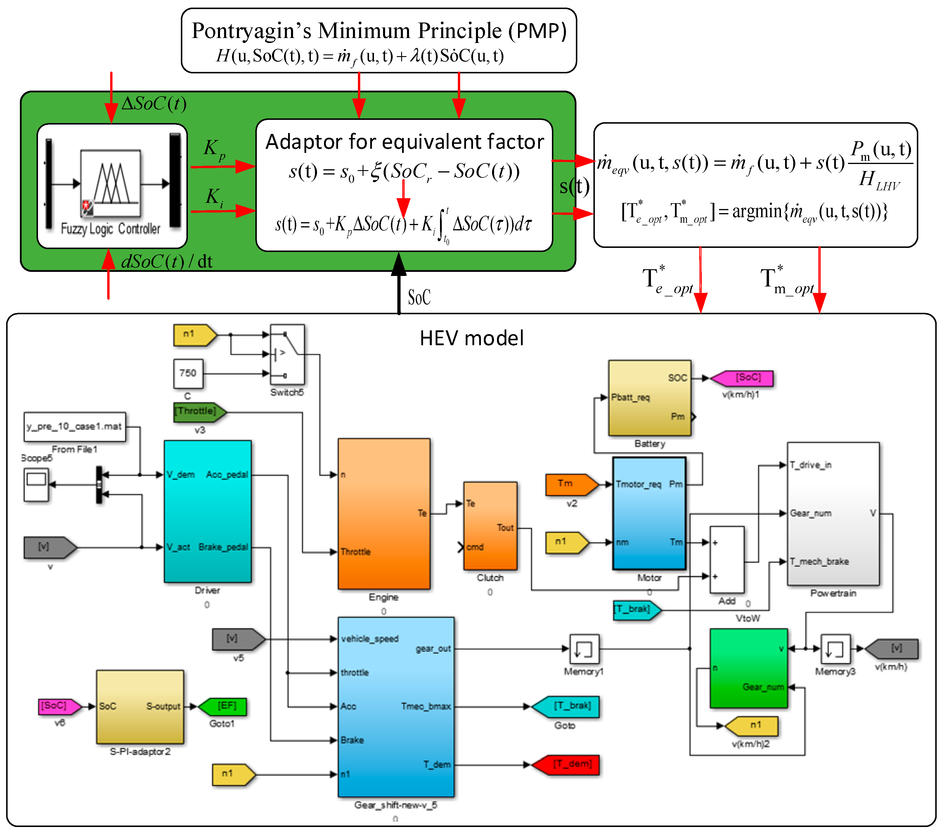
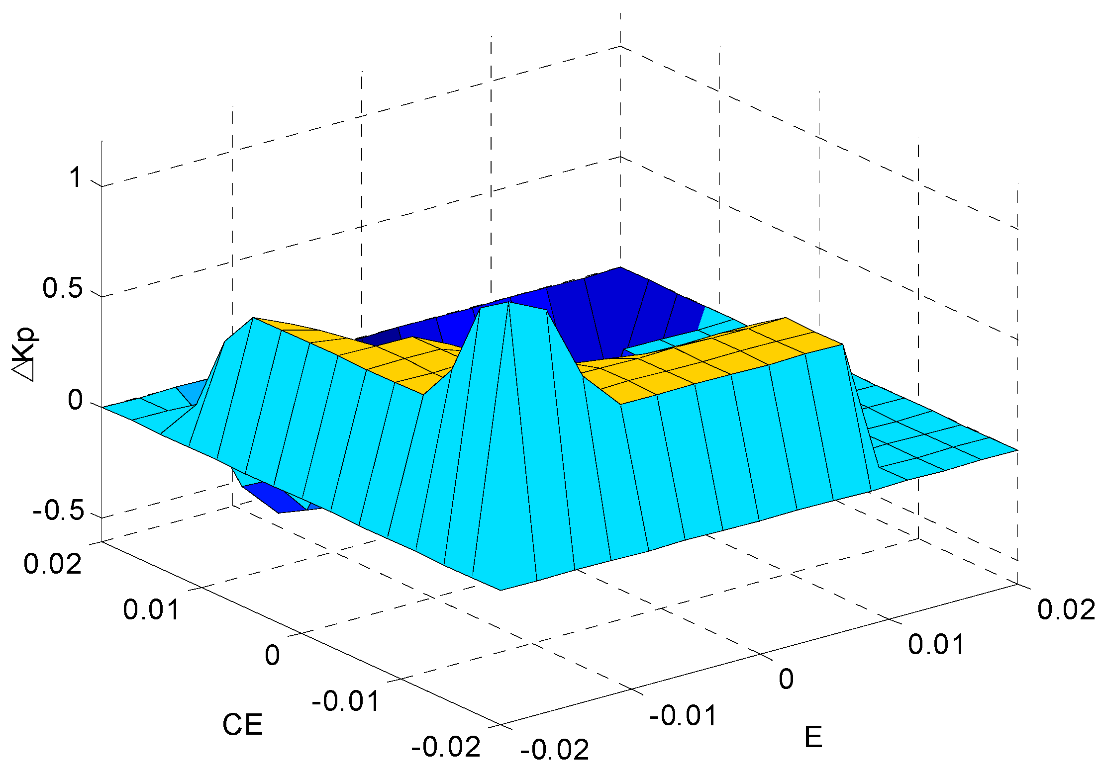
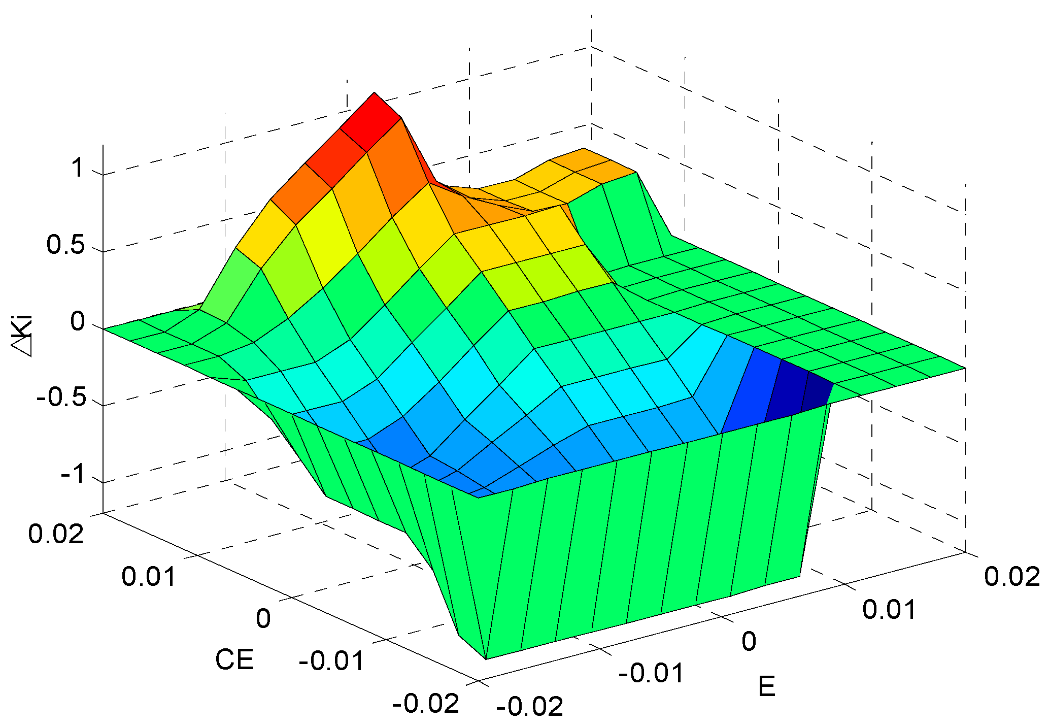
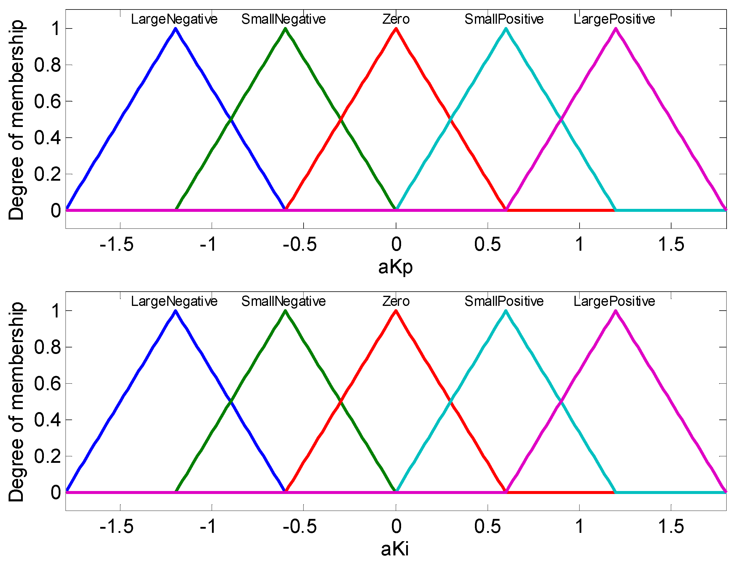
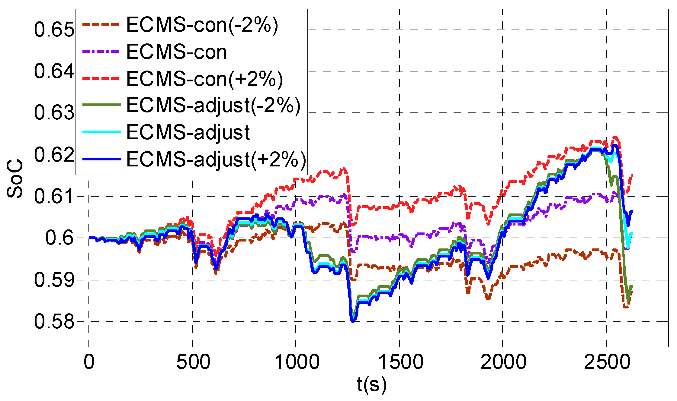
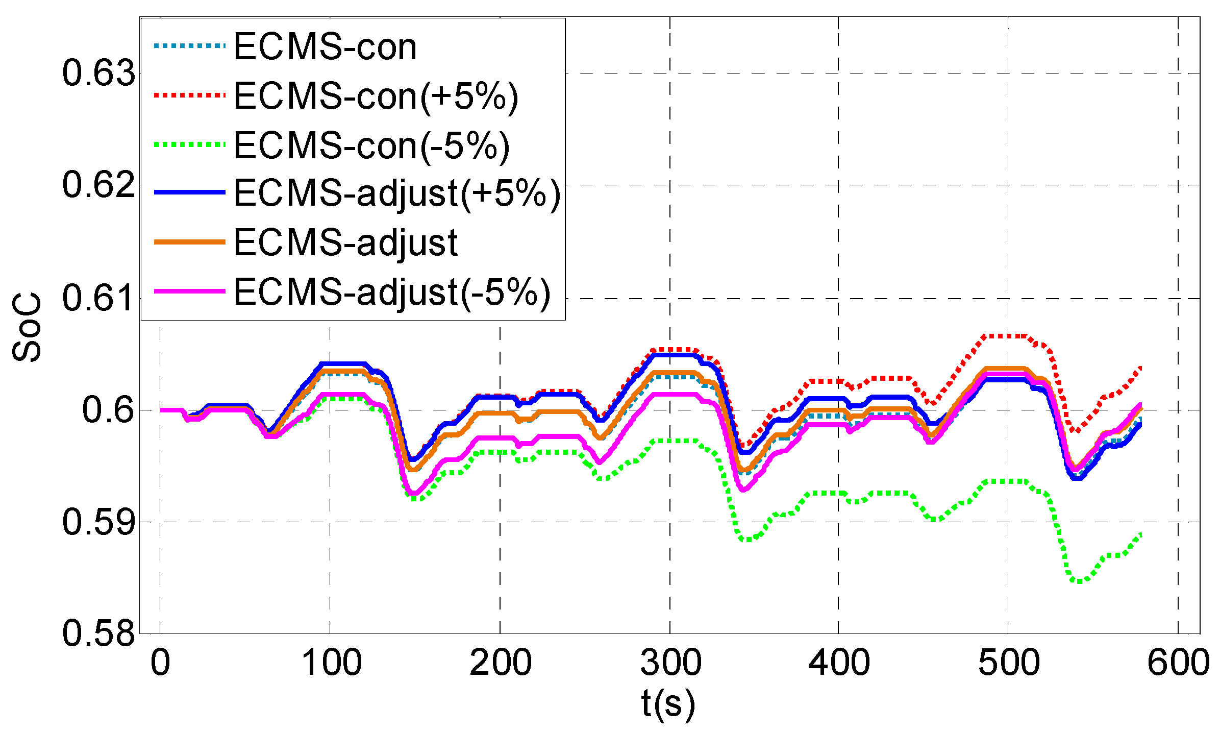
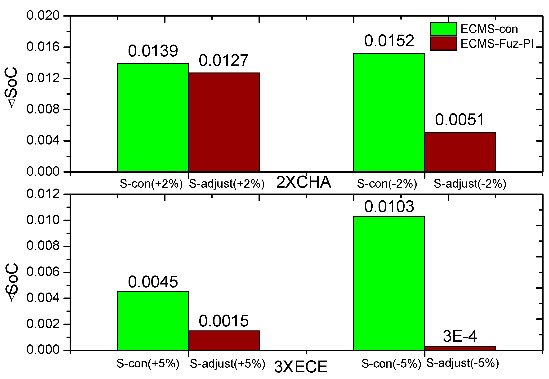
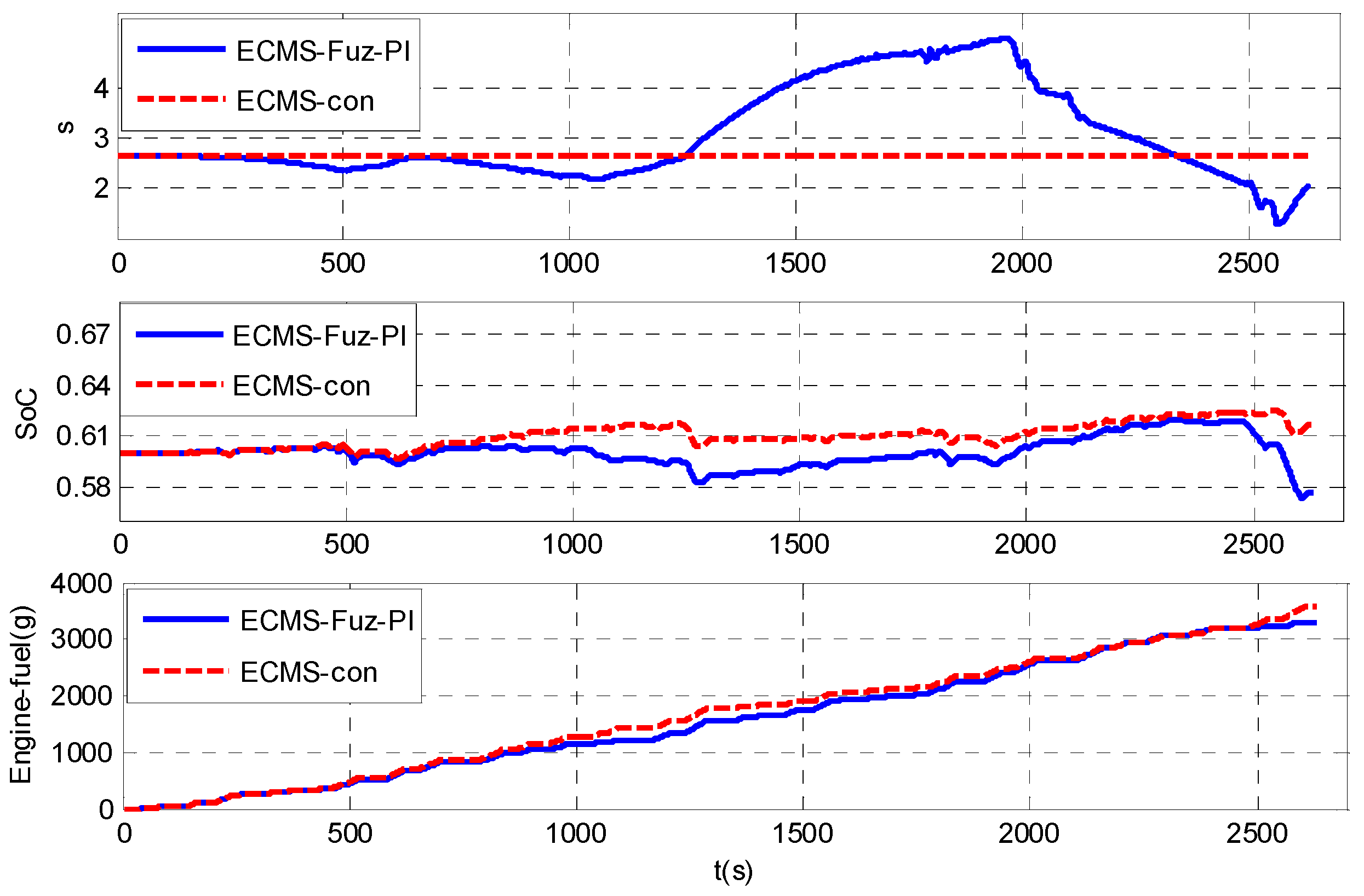
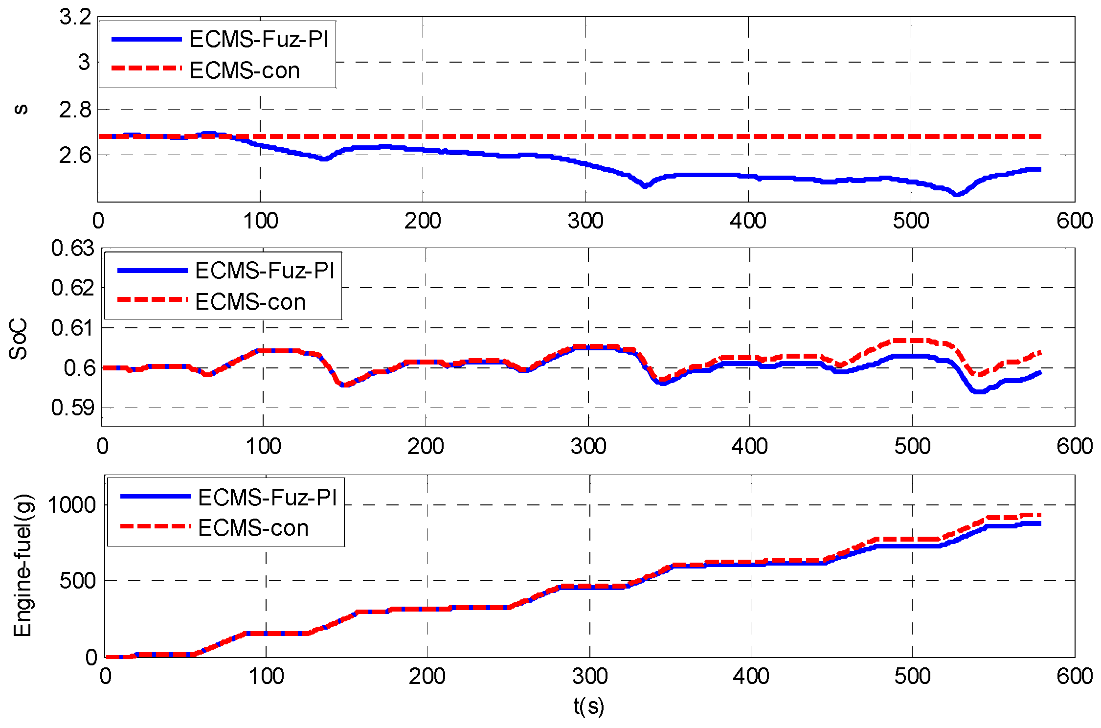
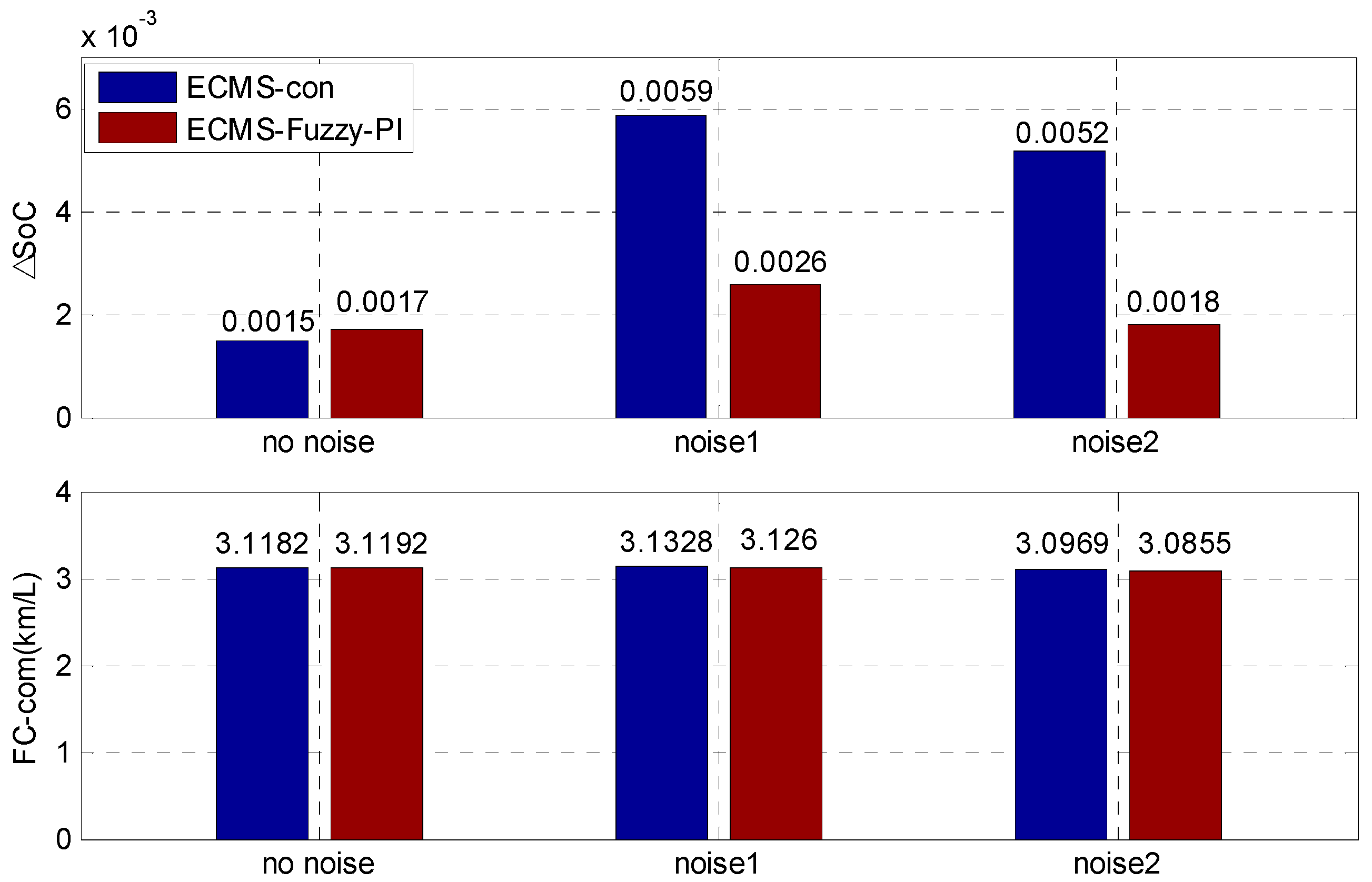
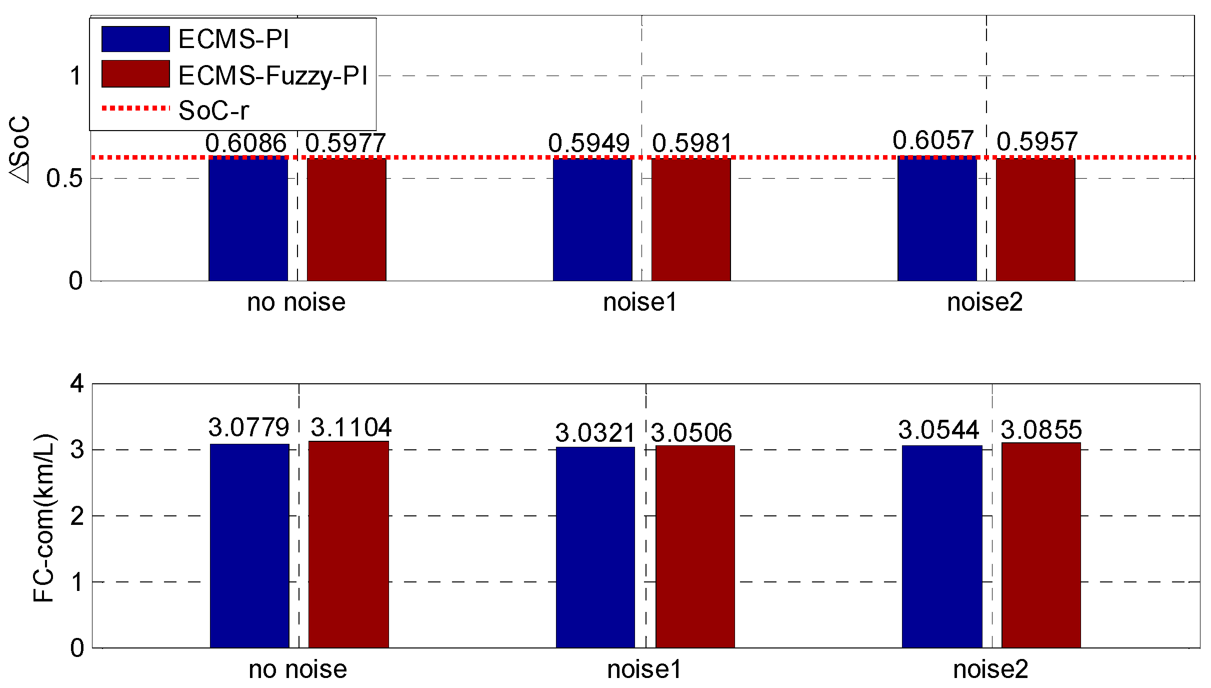
In light of this, an adaptive ECMS is proposed to improve the adaptability using a new adaptation law for different driving cycles in this paper. First, the relationship between EF of ECMS and co-state of PMP is given. Second, a new adaptation law is derived to tune the EF using a fuzzy PI controller to impose charge-sustainability and enhance robustness. The parameters of the PI are tuned dynamically by a fuzzy logic controller to improve the robustness of the adaptation law in ECMS. To our best knowledge, the second finding in this study (the adaptation law) is believed to be an original contribution. Finally, simulation results over different driving cycles are evaluated to demonstrate the effectiveness of the proposed energy management strategy compared with a rule-based control strategy. Three control strategies, namely ECMS with Fuzzy PI adaptation law, ECMS with PI adaptation law, and ECMS with constant EF, are also investigated in terms of SoC charge-sustainability and fuel economy.

The remainder of this paper is organized as follows. The system configuration and vehicle models are presented in Section 2. Section 3 introduces the energy management problem of HEVs. Section 4 proposes real-time energy management for parallel hybrid electric vehicle using a fuzzy PI controller to tune the EF applied to ECMS. In Section 5, simulation results for two driving cycles are presented and analyzed comprehensively, while conclusions are presented in Section 6.

2. System Configuration and Vehicle Modeling

2.1. System Configuration

A single-shaft parallel hybrid electric vehicle is used in this study, as shown in Figure 1. The system is composed of an engine, an automatic clutch, an electrical machine, an automated mechanical transmission (AMT), and other components. The system is simple without explicit torque couple devices, having the capability to provide six modes including motor-only, engine-only, hybrid mode, recharging mode in a driving condition, regenerative braking in hybrid mode, and regenerative braking by the motor.

2.2. Vehicle Modeling

2.2.1. Engine Model

To reduce the computational burden, the engine model can be established by a look-up table based on experimental data, which can be obtained by a bench test. The engine fuel map is shown in Figure 2. The fuel rate is a function of the engine speed and throttle. The engine maximum torque curve is presented in Figure 3. The fuel rate can be described by Equation (1) and the engine torque is formulated by Equation (2)

$${\dot{m}}_f=f(n_e,\alpha )$$

(1)

$$T_e=\alpha T_{\mathrm{emax}}(n_e)$$

(2)

where ${\dot{m}}_f$ is the engine fuel rate, $n_e$ is the engine speed, $\mathsf{\alpha }$ is the throttle opening of engine, $T_e$ is the engine torque before adding a first-order inertial link, and $T_{emax}\left(n_e\right)$ is the engine maximum torque at the current speed.

In addition, to simulate the dynamic process of the engine, a first-order inertial link is added to the output torque of engine as shown in Equation (3)

$$T_{ICE}=\frac{1}{{\tau }_{e}s+1}{T}_e$$

(3)

where ${\tau }_e$ is the coefficient for torque response and $T_{ICE}$ is the actual engine torque after adding a first-order inertial link.

Considering the engine inertia, the engine speed can be calculated by Equation (4)

$$J_e{\dot{w}}_e=T_{ICE}-T_c$$

(4)

where $J_e$ is the engine inertia, $w_e$ is the engine angular speed, and $T_c$ is the transmitted torque of the clutch.

2.2.2. Electrical Machine Model

Considering the efficiency and torque of the motor, the motor model is established by experimental data. The motor efficiency map is presented in Figure 4. The motor efficiency can be written as Equation (5), which is a function of speed and torque. The maximum and minimum torque is a function of speed as shown in Equations (6) and (7). The relationship between the actual motor torque and the required torque is described as Equation (8). The dynamic response of the torque is considered by adding a first-order inertial link as shown in Equation (9)

$${\eta }_m=\psi (n_m,T_m)$$

(5)

$$T_{max\_dis}=f_1(n_m)$$

(6)

$$T_{max\_char}=f_2(n_m)$$

(7)

$$T_m=\{\begin{array}{cc}\min (T_{m\_req},T_{max\_dis}(n_m))& T_{m\_req}>0\\ \max (T_{m\_req},T_{max\_char}(n_m))& T_{m\_req}<0\end{array}$$

(8)

$$T_{motor}=\frac{1}{{\tau }_{m}s+1}{T}_m$$

(9)

where $T_m$ is the output torque of the motor, ${\tau }_m$ is the coefficient for the torque response, $T_{m\_req}$ is the required torque of the motor (Nm), $T_{max\_dis}\left(n_m\right)$ is the maximum output torque of the motor at the current speed when the battery is discharging, $T_{max\_char}\left(n_m\right)$ is the maximum output torque of the motor at the current speed when the battery is charging, and $f_1$, $f_2$ are the efficiency functions.

In addition, the battery power is given by Equation (10)

$$P_b=\{\begin{array}{cc}\frac{T_{motor}{n}_m}{9550{\eta }_m}& T_{motor}>0\\ \frac{T_{motor}{n}_m{\eta }_m}{9550}& T_{motor}\le 0\end{array}$$

(10)

where $T_{motor}$ is the actual motor torque after adding a first-order inertial link, $n_m$ is the motor speed, ${\eta }_m$ is the motor efficiency, and $P_b$ is the required battery power.

2.2.3. Clutch Model

The clutch is used to transmit the torque to the driveline and to reduce the shock. To determine the relationship between output torque and input torque of the clutch as well as the corresponding speed, two conditions are included, as described below. Additionally, the clutch engagement is regarded to be rigidly connected since the dynamic process of the mode switch is not considered.

(1)

When the clutch is engaged or disengaged, the clutch model can be represented as Equations (11) and (12)

$$T_c=\{\begin{array}{cc}{\eta }_c{T}_e& (Clutch\_cmd=1)\\ 0& (Clutch\_cmd=0)\end{array}$$

(11)

$$w_c=\{\begin{array}{cc}{w}_e& (Clutch\_cmd=1)\\ w_m& (Clutch\_cmd=0)\end{array}$$

(12)

where $T_c$ represents the clutch transmitted torque, $T_e$ is the engine torque (Nm), ${\eta }_c$ is the clutch efficiency, $w_e$ is the engine angular velocity(rad/s), and $w_c$ is the clutch output angular velocity (rad/s). $Clutch\_cmd=1$ denotes that the clutch is engaged while $Clutch\_cmd=0$ denotes that the clutch is disengaged.

(2)

When the clutch is slipped, the input shaft speed of the clutch can be formulated by Equation (14). The transmitted torque is a function of the displacement of the clutch as shown in Equation (13) [26]. In this state, the input shaft speed of clutch is calculated by Equation (14)

$$T_c=\Psi (d_c)$$

(13)

$$w_e=w_0+{\displaystyle {\int }_{t_0}^t\frac{T_e(\upsilon )-T_c(\upsilon )}{J_e}}d\upsilon$$

(14)

where $d_c$ is the displacement of clutch, $T_c$ is the transmitted torque by the clutch, $w_0$ is the engine angular speed at instant $t_0$, $w_e$ is the engine angular speed at instant $t$, $T_e$ is the engine torque, and $J_e$ is the engine rotation inertia.

2.2.4. Battery Model

The battery model is a complicated nonlinear system, which is influenced by many factors, such as temperature, internal resistance, state of charge (SoC), and voltage, and thus it is difficult to establish a precise battery model. Some models have previously been proposed that has used some simplifications, such as Rint model, RC model, Thevenin Model, and PNGV Model [27]. The Rint model is basic and it is commonly used for energy management, which is adopted in this paper. It is assumed that the model shown in Figure 5 is equivalent to a cascade system of an ideal voltage source and a resistance. Normally, the resistance and open circuit voltage are a function of SoC, which can be represented as Equations (16) and (17).

The relationship between the terminal voltage and the open circuit voltage is formulated as Equation (15)

$$V_L=V_{oc}-I_b{R}_{in}$$

(15)

$$R_{in}=N\cdot \phi (SoC)$$

(16)

$$V_{oc}=N\cdot \psi (SoC)$$

(17)

where $N$ is the number of cells, $V_{oc}$ is the open circuit voltage, $R_{in}$ is the battery resistance, $I_b$ is the battery current, $V_L$ is the terminal voltage, and $\phi (\cdot )$ and $\psi (\cdot )$ represent the functions of open cell circuit voltage and battery resistance, respectively.

The SoC is an important parameter for energy management and it can be calculated using Equation (18) [28]

$$\frac{d}{dt}SoC=-\frac{V_{oc}-\sqrt{V_{oc}{}^2-4R_{in}{T}_m{w}_m{\eta }_m{}^{-\mathrm{sgn}(T_m)}}}{2R_{in}{Q}_{\max }}$$

(18)

where $Q_{max}$ is the maximum charging capability, $T_m$ is the motor torque, and $w_m$ is the motor speed.

Equation (18) can be rewritten in discretization form, as shown in Equation (19), to calculate the SoC at instant $k$

$$SoC(k)=SoC(t_0)+{\displaystyle {\int }_{t_0}^t(-\frac{V_{oc}-\sqrt{V_{oc}{}^2-4R_{in}{T}_m{w}_m{\eta }_m{}^{-\mathrm{sgn}(T_m)}}}{2R_{in}{Q}_{\max }}})d\tau$$

(19)

where $SoC\left(k\right)$ is the SoC value at instant $k$ and $SoC\left(t_0\right)$ is the SoC value at instant $t_0$.

In addition, the battery mainly operates in a narrow range between 0.5 and 0.7 for charge-sustaining HEVs; therefore, the resistance and open circuit voltage may not vary substantially as shown in Figure 6. Based on this fact, the resistance and open circuit voltage are considered to be constant and independent of the battery SoC.

2.2.5. Transmission Model

In this paper, the model of the gearbox and the main retarder are included. The aim of establishing the model is to determine the relationship between the output and input torque as well as the corresponding speed by taking the efficiency and the ratio of the driveline into consideration. In addition, the following assumptions were made to simplify the transmission model:

(1)

Each rotating component in the drivetrain system is considered to be rigid and is presented as a concentrated mass.

(2)

Torsional and lateral vibrations of each rotating component are ignored.

Normally, the transmission model can be formulated using Equations (20) and (21) when the gear is completely engaged

$$T_{out}=T_{in}{\eta }_G{i}_{\mathrm{g}}(G_{cu})$$

(20)

$$w_{out}=w_{in}/i_{\mathrm{g}}(G_{cu})$$

(21)

where $T_{in}$ is the torque of the transmission input shaft (Nm), $T_{out}$ is the transmission output shaft torque (Nm), $w_{in}$ is the angular velocity of the transmission input shaft (rad/s), $w_{out}$ is velocity of the transmission output shaft (rad/s), ${\eta }_G$ is the transmission efficiency, $i_g$ is the gear ratio of each transmission gear, $\mathrm{and} G_{cu}$ is the number of the current gear.

When the gear is in the neutral position, it is disengaged. The input shaft speed of transmission can be determined by Equation (22). In addition, the output shaft torque is equal to zero, as shown in Equation (23)

$$w_{in}=w_{0,in}+{\displaystyle {\int }_{t_0}^t\frac{T_{in}(\tau )}{J_{in}}}d\tau$$

(22)

$$T_{out}=0$$

(23)

where $J_{in}$ is the input shaft equivalent inertia of transmission and $w_{0,in}$ is the angular speed of the input shaft at instant $t_0$.

Due to the fixed gear ratio of the main retarder, the model can be formulated using Equations (24) and (25) by taking the efficiency and the gear ratio into consideration

$$T_f=T_{out}{\eta }_{FD}{i}_{FD}$$

(24)

$$w_{out}=w_f{i}_{FD}$$

(25)

where $T_f$ is the output torque of the main retarder, ${\eta }_{FD}$ is the efficiency of the main retarder, $i_{FD}$ is the gear ratio of the main retarder, and $w_f$ is the output angular speed of the main retarder.

2.2.6. Vehicle Dynamic Model

It is assumed that vehicle operates on a flat road; therefore, only longitudinal dynamics are considered. Lateral dynamics and handing stability are neglected. The longitudinal dynamic model for the vehicle is given by Equations (26)–(28), which are used to calculate velocity.

The vehicle drive force is shown in Equation (26)

$$F_w=F_a(\nu )+F_r+F_i$$

(26)

where $F_w$ is the drive force, $F_a$ is the air resistance, $F_r$ is the roll resistance, and $F_i$ is the acceleration resistance.

The air resistance is a function of velocity, as shown in Equation (27)

$$F_a(\nu )=\frac{c_d\cdot A_f\cdot {\nu }_a{}^2}{21.15}$$

(27)

where $c_d$ is the air resistance coefficient, $A_f$ is the frontal area, and ${\nu }_a$ is the vehicle velocity.

Thus, the longitudinal dynamic model can be rewritten as Equation (28)

$$\frac{T_w}{r_w}=\frac{c_d\cdot A_f\cdot {\nu }_a{}^2}{21.15}+m_{v}gf+\delta m_v\frac{d\nu }{dt}$$

(28)

where $m_{\nu }$ is the complete vehicle curb mass, $\delta$ is the correction coefficient of the rotating mass, $f$ is the rolling resistance coefficient, $r_w$ is the radius of the wheel, and $T_w$ is the drive torque.

The relationship between the output angular speed of transmission and the velocity is given as Equation (29)

$$w_{out}=\frac{\nu i_0}{3.6\cdot r_w}$$

(29)

where $w_{out}$ is the output angular speed of transmission and $i_0$ is the gear ratio of the main retarder.

2.2.7. Driver Model

To track the velocity of the driving cycle, the driver model is adopted to determine the values of acceleration and deceleration in the forward simulation. The proportion integral derivative (PID) driver model formulated in Equations (30) and (31) is commonly used. The structure of the PID driver model is shown in Figure 7.

$$e=v_{dem}-v_{act}$$

(30)

$$u_{\mathrm{PID}}=K_{p}e+K_i{\displaystyle {\int }_0^{t}edt+K_d}\frac{de}{dt}$$

(31)

where $u_{\mathrm{PID}}$ $\in \left[-11\right]$, with $u_{\mathrm{PID}}$ $<0$ representing the driver braking and $u_{\mathrm{PID}}$ $>0$ representing the driver accelerating. $K_p$, $K_i$, $K_d$ are the proportional, integral, derivative coefficients of the PID driver model, respectively, which are determined by trial and error. $v_{dem}$ is the demand velocity and $v_{act}$ is the actual velocity.

3. Problem Statement

The goal of HEVs energy management is to distribute the power between the internal combustion engine (ICE) and the electrical machine (EM), given the driver’s total power demand, while aiming to minimize fuel consumption. The energy management of HEVs is commonly regarded as an optimal control problem, aiming to find an optimal power split between the engine and the motor under various soft and hard constraints. Note that the power distribution is converted into the torque split due to the system configuration in this paper.

The cost function can be written as Equation (32), which is an optimization objective for the energy management problem in HEVs. The first term is fuel consumption and the second term is used to attain SoC charge-sustainability

$$J(SoC(t))={\displaystyle {\int }_{t_0}^{t}L(u,t)}dt+\beta {(SoC(t)-So{C}_r)}^2$$

(32)

$$\{T_e^{opt},T_m^{opt}\}=\mathrm{argmin}\{J(SoC(t))\}$$

(33)

where $J\left(SoC\left(t\right)\right)$ is the cost function from $t_0$ to $t$, $u$ is the control input, such as engine torque and motor torque, $\beta$ is the penalty coefficient, $SoC\left(t\right)$ is the current SoC at instant $t$, and $So{C}_r$ is the reference SoC.

ECMS, as a real-time optimization method, aims at minimizing instantaneous fuel consumption by converting the electrical power into the equivalent fuel consumption to obtain the optimal solution. Thus, the equivalent factor (EF) is needed to convert the motor power into equivalent fuel consumption. The challenge in implementing ECMS is that the optimal solution is sensitive to the EF, which can be appropriately determined only if the whole driving cycle is known; however, this is impossible under real conditions. Thus, it is necessary to adjust the EF online. The basic principle of ECMS is illustrated as follows.

The instantaneous fuel consumption of ECMS is given in Equation (34)

$${\dot{m}}_{eqv}(u(t),t)={\dot{m}}_f(u(t),t)+{\dot{m}}_e(u(t),t)={\dot{m}}_f(u(t),t)+s(t)\frac{P_m(u(t),t)}{H_{LHV}}$$

(34)

where ${\dot{m}}_{eqv}\left(u\left(t\right),t\right)$ is the equivalent fuel consumption, ${\dot{m}}_f\left(u\left(t\right),t\right)$ is the engine fuel mass flow (kg/s), ${\dot{m}}_e\left(u\left(t\right),t\right)$ is the equivalent fuel by converting the motor power into fuel consumption (kg/s), $s$(t) is the equivalent factor (EF), $P_{m }\left(u\left(t\right),t\right)$ is the motor power (kW), and $H_{LHV}$ is the fuel lower heating value (kJ/kg). The optimal solution should be subjected to the constraint conditions shown as Equation (35)

$$\begin{array}{l}{T}_{dem}(t)=T_e(t)+T_m(t)\\ T_{m\_\min }(w_m(t))\le T_m(t)\le T_{m\_\max }(w_m(t))\\ 0\le T_e(t)\le T_{e\_\max }(w_e(t))\\ 0\le w_m(t)\le w_{m\_\max }\\ w_{e\_\min }\le w_e(t)\le w_{e\_\max }\\ So{C}_{\min }\le SoC(t)\le So{C}_{\max }\end{array}$$

(35)

where $T_e^{opt} \mathrm{and} T_m^{opt}$ are the optimal engine and motor torques, respectively, $T_{dem}\left(t\right)$ is total torque demand(Nm), $T_e\left(t\right)$ is the engine torque, $T_m\left(t\right)$ is the motor torque, $T_{m\_max}\left(w\left(t\right)\right)$ is the motor maximum torque, $T_{m\_min}\left(w_e\left(t\right)\right)$ is the motor minimum torque, $T_{e\_max}\left(w_e\left(\mathrm{t}\right)\right)$ is the engine maximum torque, $w_m\left(t\right)$ is the motor speed, $w_{m\_max}$ is the motor maximum speed, $w_e\left(t\right)$ is the engine speed, $w_{e\_min}$ is the engine minimum speed, $w_{e\_max}$ is the engine maximum speed, $So{C}_{min}$ is the minimum SoC, and $So{C}_{max}$ is the maximum SoC.

The aim of the optimal control algorithm is to obtain the ideal power-split and to ensure SoC charge-sustainability over a whole cycle. Figure 8 shows the SoC trajectory for charge-sustaining HEVs.

From the above analysis, we can see that the key problem is how to adjust the EF to ensure optimal performance of ECMS.

4. The Proposed Energy Management of HEVs

4.1. Equivalent Consumption Minimization Strategy (ECMS)

To improve the optimal performance of ECMS, the principle used to adjust the EF is derived as follows. It is well known that pontryagin’s minimum principle (PMP) can give a better understanding of the ECMS to determine the optimal EF. The Hamiltonian function for the cost objective is expressed as Equation (36)

$$H(u(t),SoC(t),t,\lambda (t))={\dot{m}}_f(u(t),t)+\lambda (t)S\dot{o}C(t)$$

(36)

where $\lambda (t)$ is the co-state, according to the principle of PMP, and the co-state dynamic equation can be given as Equation (37) [29].

$$\dot{\lambda }(t)=-\frac{\partial H(u(t),SoC(t),t,\lambda (t))}{\partial SoC(t)}=-\lambda (t)\frac{\partial S\dot{o}C(t)}{\partial SoC(t)}$$

(37)

According to the Equation (18), we can derive Equation (38) since the battery mainly operates in a narrow range for charge-sustaining HEVs, e.g., from 0.5 to 0.7 [30], and the voltage and resistance remain constant, as explained in Section 2.

$$\dot{\lambda }(t)=0$$

(38)

This denotes that $\lambda \left(t\right)$ is constant and the optimal co-state ${\lambda }^{*}(t)$ should satisfy the SoC boundary condition as Equation (39)

$$SoC(t_f)=SoC(t_0)$$

(39)

where $t_0$ and $t_f$ are the start and end times of the driving cycle, respectively.

The SoC can be expressed as Equation (40).

$$SoC(t)=-\frac{Q}{Q_{\max }}=-\frac{1}{Q_{\max }}{\displaystyle {\int }_0^t{I}_b(\tau )d\tau }$$

(40)

We can derive Equation (41) by deriving Equation (40).

$$S\dot{o}C(t)=-I_b/Q_{\max }$$

(41)

The battery current can be expressed as Equation (42).

$$I_b=P_m(u(t),t)/V_{oc}$$

(42)

We can substitute Equation (42) into Equation (41) and the Equation (41) can be rewritten as

$$S\dot{o}C(t)=-P_m(u(t),t)/V_{oc}{Q}_{\max }$$

(43)

then the Equation (43) is substituted into Equation (36) and Equation (36) can be rewritten as

$$H(u(t),SoC(t),t,\lambda (t))={\dot{m}}_f(u(t),t)-\frac{\lambda (t)H_{LHV}}{Q_{\max }{V}_{oc}}\frac{P_m(u(t),t)}{H_{LHV}}$$

(44)

By comparing Equation (34) with Equation (44), it was found that

$$s(t)=-\frac{\lambda (t)H_{LHV}}{Q_{\max }{V}_{oc}}$$

(45)

Thus, it may be observed that the challenge in finding the EF depends on the value of the co-state in Equation (45). However, the optimal co-state may vary for different driving cycles and it strongly depends on the future driver’s power demand, while satisfying the SoC boundary in Equation (39). Therefore, the optimal value of $s\left(t\right)$ depends on the future driver’s power demand as well as the current value of SoC.

According to the Hamilton-Jacobi-Bellman equation, we know that the corresponding optimal co-state ${\lambda }^{*}(t)$ [12], is equal to

$${\lambda }^{*}(t)=\frac{\partial J(SoC(t))}{\partial SoC(t)}$$

(46)

To impose SoC charge-sustainability, the cost function can be rewritten as

$$J(SoC(t))={\displaystyle {\int }_{t_0}^t{\dot{m}}_f(u(t),t)}dt+\eta \frac{Q_{\max }}{H_{LHV}}{\displaystyle {\int }_{SoC(t_0)}^{SoC(t)}{V}_{oc}}d(1-SoC)+\beta {(So{C}_r-SoC(t))}^2$$

(47)

where $So{C}_r$ is the SoC reference value and $So{C}_r-SoC\left(t\right)$ is the difference between the reference SoC and the actual SoC value. $\eta ={\eta }_m/{\eta }_e$, $\mathrm{where}{\eta }_m$ is the average motor efficiency and ${\eta }_e$ is the average engine efficiency. The first term of Equation (47) is the engine fuel consumption, which is independent of the battery SoC. The second term represents the equivalent fuel consumption by converting the motor power and the third term is a penalty function to impose battery charge-sustainability. Thus, we can derive Equation (48) by taking the derivative of Equation (47) with respect to SoC.

$${\lambda }^{*}(t)=\frac{\partial J(SoC(t))}{\partial SoC(t)}=-\eta \frac{Q_{\max }{V}_{oc}}{H_{LHV}}-2\beta (So{C}_r-SoC(t))$$

(48)

Combining Equations (45) and (48), the equivalent factor can be derived as Equation (49).

$$s(t)=\eta +2\beta \frac{H_{LHV}}{Q_{\max }{V}_{oc}}(So{C}_r-SoC(t))$$

(49)

Equation (49) is composed of two parts. The first term represents the efficiency of the motor and engine while the second term is related to the difference between the reference SoC and the actual SoC. To impose charge-sustainability effectively, we can obtain the law describing how to adjust the EF by replacing Equation (49) with Equation (50)

$$s(t)=s_0+K_p(So{C}_r-SoC(t))+K_i{\displaystyle {\int }_{t_0}^t(So{C}_r-SoC(\upsilon ))d\upsilon }$$

(50)

where $s_0$ is the initial value (constant) and $K_p$ and $K_i$ are the proportional and integral coefficients, respectively.

When the value of $s\left(t\right)$ is determined, ECMS is used to obtain the optimal torque-split as Equation (51)

$$[T_{e\_opt}^{*},T_{m\_opt}^{*}]=\mathrm{argmin}\{{\dot{m}}_{eqv}(u(t),t,s(t))\}$$

(51)

where $T_{e\_opt}^{*}$ and $T_{m\_opt}^{*}$ are the optimal engine torque and motor torque, respectively.

4.2. Adjust the Equivalent Factor

As Equation (50) indicates, the key problem is deciding how to adjust the parameters $K_p$ and $K_i$ of the adaptation law of EF, which is illustrated as follows.

4.2.1. Estimating the EF

To determine the approximate optimal EF in an effective way, an iterative method is adopted to calculate the EF. Thus, we propose the following specific steps. It is noted that this method requires prior knowledge of the driving cycle. In this paper, we use a standard driving cycle for simulations to demonstrate the effectiveness of the proposed strategy. However, since the full driving cycle is not known in real conditions, we can choose the average efficiency ($\eta ={\eta }_m/{\eta }_e$) as the initial EF for the adaptation law.

Step 1: Estimate the range of EF and select the initial value as a first try to obtain the SoC trajectory.

Step 2: Discretize the range of EF at a fixed step to obtain a series of EF values.

Step 3: Calculate the SoC trajectory for each EF according to the vehicle model as well as ECMS and obtain the final SoC value.

Step 4: Check the final SoC of each trajectory and select the value of EF that satisfies the boundary condition (Equation (52)). The optimal SoC trajectory is also obtained accordingly

$$SoC(t_0)=SoC(t_f)$$

(52)

where $t_0 \mathrm{and}{t}_f$ are the initial and final times of the driving cycle, respectively.

The specific flowchart describing the methods used to determine the initial EF is presented in Figure 9.

It is noted that the boundary condition is not strictly held in some cases due to the choice of the discretization step. In light of this, we need to set up a soft constraint, as illustrated in Equation (53), to determine the EF

$$So{C}_{new\_f}=SoC(t_0)\pm \Delta SoC$$

(53)

where $So{C}_{new\_f}$ is the new final value after correction.

Normally, the choice of $\Delta SoC$ is related to the driving cycle and discretization step. In this paper, $\Delta SoC$ is selected as 0.02. On the other hand, the EF obtained from the iterative method cannot be directly applied in real conditions due to variation in the driving cycle. Hence, it is necessary to adjust the EF online based on the variation of SoC.

4.2.2. Adjust the EF

A PI controller is adopted to adjust the EF of ECMS for plug-in HEVs [14]; however, the methods used to tune the parameters of the PI controller are not given to impose SoC charge-sustainability for HEVs. Thus, we emphasize the adjustability of EF using a fuzzy PI controller in this section.

To impose charge-sustainability and improve fuel economy, the EF needs to be tuned online. In view of this, a new adaptation law based on a fuzzy PI controller is devised. The error (E) between the SoC reference value and its actual value along with the derivative of this error (CE) are selected as inputs of a fuzzy inference system. We define five linguistic values for inputs and outputs, namely “Large Negative” (NL), “Small Negative” (NS), “Zero” (ZO), “Small Positive” (PS), and “Large Positive” (PL). In addition, different membership functions may produce distinct results. However, we mainly focus on the adjustment of PI parameters instead of optimizing membership function in this paper. Thus, we select the Triangular Membership function that is commonly used [31,32]. The range of inputs and outputs is determined as (−0.02, 0.02) and (−1.8, 1.8), respectively, after completing the testing. Based on these parameters, a fuzzy logic controller is devised to adjust the values of $K_p$ and $K_i$ dynamically. Based on the new adaptation law, the proposed energy management is illustrated in Figure 10. As can be seen from Figure 10, the first step is to derive the EF applied in ECMS from the PMP based on the analysis of the battery SoC operating range, as shown in Section 2. In the next step, the new adaptation law applied in ECMS based on fuzzy PI is proposed to improve robustness. Finally, the optimal power-split can be obtained by ECMS to implement energy management.

The output of the fuzzy inference system for $\Delta K_p$ and $\Delta K_i$ is shown in Figure 11 and Figure 12, respectively. The membership functions for the inputs and outputs are shown as Figure 13. The fuzzy rules of $\Delta K_p$ and $\Delta K_i$ are presented in

Table 1. The fuzzy rule of $\Delta K_p$.

	CE	NL	NS	Zero	PS	PL
E
NL		PL	PS	PS	PS	ZO
NS		PS	PS	PS	ZO	NS
Zero		PS	PS	ZO	NS	NS
PS		PS	ZO	NS	NS	NL
PL		ZO	ZO	NS	NS	NL

and

Table 2. The fuzzy rule of $\Delta K_i$.

	CE	NL	NS	Zero	PS	PL
E
NL		NL	N	NS	NS	ZO
NS		NL	NS	NS	ZO	PS
Zero		NL	NS	ZO	PS	PL
PS		NS	ZO	PS	PS	PL
PL		ZO	ZO	PS	PS	PL

, respectively. The values of $K_p$ and $K_i$ can be expressed as Equations (54) and (55).

$$K_p=K_{p0}+\Delta K_p$$

(54)

$$K_i=K_{i0}+0.5\Delta K_i$$

(55)

5. Simulation Results and Discussion

5.1. SoC Trajectory

To evaluate the performance of the proposed fuzzy PI controller, two strategies, namely ECMS with constant EF and with the fuzzy PI controller, are conducted and compared. Figure 14 and Figure 15 present the SoC trajectory using these two methods for the 2 × CHA (two CHA cycles) and 3 × ECE (three ECE cycles) cycles, respectively. The initial value of SoC is set as 0.6, and the initial values of $K_{p0}$ and $K_{i0}$ are chosen as 5 and 0.5, respectively. Moreover, to make a fair comparison of the optimal ECMS (ECMS-con) and Fuzzy-PI-ECMS, we choose the approximate optimal EF (obtained from the iterative method described in Section 4.2.1) as the initial value for the Fuzzy-PI ECMS. The approximate optimal EF are chosen as 2.58 and 2.555 for 2 × CHA and 3 × ECE, respectively. As for the real condition, we can choose the average efficiency ($\eta ={\eta }_m/{\eta }_e$) as the initial EF for the fuzzy-PI-ECMS. The average efficiency is not always equal to the optimal EF. To further demonstrate the adaptability of the fuzzy PI for ECMS, deviations ($\pm$2% for the 2 × CHA cycle and$\pm$5% for the 3 × ECE cycle) are added to the approximate optimal EF (ECMS-con) for two strategies as well since it is difficult to obtain the exact optimal EF. Normally, the difference between the exact optimal EF and the estimated EF exists. As for ECMS-fuzzy PI, deviations are added to the initial EF. Note that the optimal EF is obtained from the iterative method to satisfy the SoC boundary, as described in [13].

As can be seen in Figure 14 and Figure 15, the SoC trajectory obtained from the fuzzy PI controller is almost consistent even though different values of EF are selected for the 2 × CHA cycle. However, the trajectories differ substantially when EF is chosen as different value using ECMS with a constant EF. Similarly, the deviation of the SoC trajectory using ECMS with the fuzzy PI controller is smaller than that generated by ECMS with a constant EF for the 3 × ECE cycle. This verifies that the new adaptation law can adjust the EF efficiently and it is more robust for ECMS with a constant EF.

A comparison of SoC deviations for two control strategies is also presented in Figure 16. The maximum and minimum SoC deviations for the ECMS-Fuzzy-PI are 0.0127 and 0.0003, respectively, while they are 0.0152 and 0.0045, respectively, for ECMS-con. It is found that the same deviation of the equivalent factor leads to a substantial difference. The SoC deviation of ECMS with a fuzzy PI controller is observed to be smaller than that of ECMS with a constant EF. The final SoC value of ECMS with a fuzzy PI controller shows improved convergence to the reference value. This also confirms the capability of the proposed fuzzy PI controller to impose SoC charge-sustainability.

5.2. Fuel Consumption

To assess the performance of the proposed control strategy, the fuel consumption for a hybrid electric bus is calculated by ECMS. The vehicle configuration is shown in

Table 3. The vehicle configuration.

Component	Parameter	Value
Engine	Maximum Power (kW)	125
	Maximum Torque (Nm)	600
	Maximum speed (r/min)	2600
Motor	Maximum Power (kW)	150
	Maximum Torque (Nm)	650
	Nominal speed (r/min)	2600
Transmission	AMT gear ratio	[6.25, 3.583, 2.22, 1.36, 1, 0.74]
	Final gear ratio	6.17
Battery	Cell open circuit voltage (V)	3.8
	Capacity (Ah)	70
	Voltage (V)	650
Vehicle	Mass (kg)	18,000
	Roll coefficient	0.01
	Cd	0.65
	A	6.73
	Radius (m)	0.5715
	$\mathsf{\delta }$	1.04

. In addition, to obtain a fair comparison for different control strategies, we use the SoC compensated fuel consumption, which is calculated by Equations (56) and (57)

$$E_{\Delta SoC}=(So{C}_f-So{C}_0)\cdot N_{cell}\cdot Q_{max}\cdot 3600{\displaystyle \int U_{ocv\_disch\arg e}d(1-SoC)}$$

(56)

$$F{C}_{\Delta SoC\_comp}=\frac{FC-\frac{E_{\Delta SoC}}{E_{diesel}{\eta }_{diesel}{\eta }_{ICE}{\eta }_{EM}}}{{\rho }_{diesel}{d}_{cycle}\cdot {10}^{-5}}$$

(57)

where $E_{\Delta SoC}$ is the energy produced by the SoC deviation (J), $So{C}_f$ and $So{C}_0$ are the final and initial values of SoC, respectively, $N_{cell}$ is the number of cells in the battery, $Q_{max}$ is the capacity of the battery (Ah), $U_{ocv\_discharge}$ is the cell voltage (V), $F{C}_{\Delta SoC\_comp}$ is the SoC compensated fuel consumption (L/100 km), $FC$ is the fuel consumption before compensation (kg), $E_{diesel}$ is the energy content of the diesel fuel (J/kg), ${\eta }_{diesel}$ is the efficiency of the conversion from diesel energy to electricity, ${\eta }_{ICE}$ is the diesel engine efficiency, ${\eta }_{EM}$ is the motor efficiency, ${\rho }_{diesel}$ is the density of diesel (0.84 kg/L), and $d_{cycle}$ is the distance traveled (m).

Table 4. Comparison of performances of different control strategies.

Driving Cycle	Performance Index	ECMS-Con			ECMS-Fuz-PI			A-ECMS
		ECMS-Con	ECMS-Con (+2%/+5%)	ECMS-Con (−2%/−5%)	ECMS-Adjust	ECMS-Adjust (+2/+5%)	ECMS-Adjust (−2%/−5%)	ECMS-Adjust	ECMS-Adjust (+2%/+5%)	ECMS-Adjust (−2%/−5%)
2 × CHA	$So{C}_{final}$	0.601	0.6149	0.5858	0.6012	0.5885	0.6063	0.5913	0.5892	0.5913
	$|\Delta$SoC|	0	0.0139	0.0152	0	0.0127	0.0051	0	0.0021	0
	FC_com (km/L)	2.886	2.818	2.945	2.795	2.824	2.777	2.747	2.749	2.746
3 × ECE	$So{C}_{final}$	0.5992	0.6037	0.5889	0.6002	0.5987	0.6005	0.5934	0.5937	0.5928
	$|\Delta$SoC|	0	0.0045	0.0103	0	0.0015	0.0003	0	0.0003	0.0006
	FC_com (km/L)	2.844	2.750	3.065	2.813	2.851	2.815	2.814	2.807	2.823

summarizes the fuel consumption as well as the SoC deviation over two driving cycles. As can be seen in Table 4, the fuel consumptions of ECMS-con and ECMS-Fuzz-PI are 2.818 km/L and 2.824 km/L over a 2 × CHA cycle, respectively, when the optimal value of EF is increased. Similarly, the fuel consumptions are 2.750 km/L and 2.851 km/L for a 3 × ECE cycle, respectively. When the optimal EF is increased, the fuel economies of ECMS-Fuzz-PI are improved by 0.2% and 3.6%, while those of ECMS-con have less substantial improvements. In contrast, the ECMS with constant EF can achieve a better fuel economy if the optimal EF is selected. However, this cannot be guaranteed because of variation of the parameters and the driving cycle. To further demonstrate the effectiveness of the proposed strategy, the adaptation law in [18] (A-ECMS) is implemented as well. It can be seen that both ECMS-Fuzz-PI and A-ECMS can adjust the EF efficiently. The only difference is that the adaptive ECMS [18] results in greater fuel consumption than the proposed strategy for the 2 × CHA cycle. The reason may be that A-ECMS only adopts the proportional law and is not as steady as Fuzzy-PI-ECMS for different driving cycles.

Thus, the ECMS fuzzy PI can give a better performance in adjusting EF, especially when the EF is not optimal. Another interesting phenomenon is that the fuel consumption using ECMS with fuzzy PI is slightly higher than that with constant EF when the optimal EF decreases. This is because more charging behaviors are performed by the engine to impose charge-sustainability for ECMS-Fuzz-PI while for ECMS-con, the solution is charge-depleting when the EF is smaller than the optimal value. However, the fuel economy does not deteriorate much compared to the optimal fuel consumption. In conclusion, the ECMS-Fuzz-PI provides a promising blend in terms of fuel economy and charge-sustainability. To obtain a fair comparison and to demonstrate the effectiveness of the optimal algorithm, we perform a simulation of rule-based control (RB) strategy.

Table 5. Comparison of different control strategies.

Driving Cycle	2 × CHA			3 × ECE
Index	FC_com (km/L)	SoC_final	FC Improvement	FC_com (km/L)	SoC_final	FC Improvement
RB	2.676	0.5999	0	2.453	0.589	0
ECMS-Fuz-PI	2.795	0.6012	4.44%	2.813	0.6002	14.7%

Note: FC_com: SoC compensated fuel consumption.

summarizes the fuel consumption of two control strategies, showing that the fuel economy through ECMS-Fuzz-PI improves by 4.44% and 14.7% compared with RB over the 2 × CHA and 3 × ECE cycles, respectively.

5.3. Performance of Adjusting EF

To demonstrate the performance of the fuzzy PI, the evolution of EF as well as SoC over the 2 × CHA and 3 × ECE cycles are presented in Figure 17 and Figure 18, respectively.

As it may be observed from Figure 17, the EF of ECMS-Fuzz-PI is changing with varying SoC over the 2 × CHA cycle, resulting in variation in SoC to impose SoC charge-sustainability. The scope of EF using the fuzzy PI controller involves reacting to these changes of SoC and therefore the fuel consumption is reduced. Specifically, the EF is gradually increased to encourage the use of the engine torque to charge the battery starting from 1200 s to 1700 s and then the EF decreases at about 2000 s when the SoC reaches the reference value. In contrast, the solution is charge-increasing for the reference SoC value when the EF remains constant over the entire driving cycle, resulting in an increase of fuel consumption.

Similarly, the effects of adjusting the EF on performance for the 3 × ECE cycle are shown in Figure 18. The effect on performance is not as strong as for the 2 × CHA cycle because the deviation of SoC is small during the whole cycle. Thus, using the Fuzzy PI controller, the changes in EF are small. In contrast, the solution is charge-increasing using a constant EF. This indicates that the proposed adaptation law can adjust the EF according to variation of the SoC rather than remaining constant over the entire cycle. In conclusion, the proposed adaptation law using Fuzzy PI achieves better performance in terms of fuel economy and charge-sustainability.

To further evaluate the advantage of ECMS compared to RB, the engine operation point for two control strategies for a 2 × CHA cycle are shown in Figure 19 and Figure 20. It can be seen from Figure 19 and Figure 20 that most engine operating points are concentrated in the lower fuel consumption region for ECMS while part of that is located beyond the lowest fuel consumption region for RB. This is because the power is distributed by minimizing the instantaneous fuel consumption for ECMS to ensure the engine is operating in its lowest fuel consumption region, but the RB cannot guarantee optimality at each time step.

Figure 21 and Figure 22 present the motor operation point for ECMS and for the rule-based control strategy, respectively. It may be observed that most of the motor operation points are concentrated in higher efficiency region for ECMS; however, fewer points are located in that region for the RB. This also confirms that ECMS would be capable of providing better fuel economy than RB due to its optimality. The red and pink circles represent the motor operation points in Figure 21 and Figure 22.

5.4. Robustness to Driving Cycles

To further evaluate the robustness of the proposed Fuzzy PI adaptation law, simulations are conducted using the optimal EF applied in ECMS by adding variation to the driving cycle. In this paper, two kinds of noise signal are considered, as shown in Figure 23 and Figure 24. The comparison of fuel consumption along with final SoC over the 2 × CHA cycle is shown in Figure 25. We compare the performance of the approximate optimal EF applied in ECMS (ECMS-con) and the Fuzzy-PI adaptation law in ECMS (ECMS-Fuzzy-PI).

As shown in Figure 25, the deviation between the final SoC and the reference value is almost the same when no noise signal is added to the driving cycle, reaching 0.0015 and 0.0017 for ECMS-con and ECMS-Fuzzy-PI, respectively. Both ECMS-con and ECMS can achieve better performance in terms of fuel economy and charge-sustainability. In contrast, the SoC deviation of ECMS-con increases, with values of 0.0059 and 0.0052 for Noise1 and Noise2, respectively, when variations are added to the driving cycle. However, the final SoC can be better guaranteed with ECMS-Fuzzy-PI, resulting in smaller SoC deviation. On the other hand, the fuel consumption of ECMS-Fuzzy-PI is slightly higher than that with ECMS-con, with values of 3.126 km/L and 3.0855 km/L for Noise1 and Noise2, respectively. These results verify that the final SoC using ECMS-con cannot better converge to the reference value due to the variation of driving cycle and the ECMS-Fuzzy-PI controller provides a better performance in terms of charge-sustainability and fuel economy. In conclusion, ECMS-Fuzzy-PI is more robust than ECMS-con and it better adapts to the driving cycle. The proposed energy management system is more feasible for real-time control than ECMS with constant EF.

To better demonstrate the adjustability of the proposed Fuzzy PI adaptation law, simulation of the PI controller and the Fuzzy PI controller applied in ECMS to adjust the EF are also conducted. The comparison of the final SoC as well as the fuel consumption over a 2 × CHA cycle is shown in Figure 26. Note the parameter of PI ($K_{p0}=5$, $K_{i0}=0.05$) remains the same for the three cases.

As can be seen from Figure 26, the solution of ECMS-PI is charge-increasing and SoC deviation is 0.0086 when no noise is added to the driving cycle, but the SoC deviation is only 0.0023 using ECMS-Fuzzy-PI. On the other hand, the fuel consumption is lower than one with ECMS-PI. In addition, SoC deviations using ECMS-Fuzzy-PI, which are only 0.0019 and 0.0043 for Noise1 and Noise2, respectively, are smaller than those with ECMS-con, (0.0051 and 0.0057 for Noise1 and Noise2, respectively). Similarly, the fuel economy is better compared to ECMS-PI, though the noise signal is added to driving cycle. This demonstrates that ECMS-Fuzzy-PI is more robust than ECMS-PI and it can better guarantee the final constraint of SoC even though velocity noise is added to driving cycle. Moreover, the ECMS-Fuzzy-PI controller can effectively adjust the parameters of the PI adaptation law applied in ECMS. In conclusion, ECMS-Fuzzy-PI is capable of imposing the SoC charge-sustaining condition and improving the fuel economy, even if variations are added to driving cycle.

6. Conclusions

A new energy management system for parallel hybrid electric vehicles is proposed based on the Fuzzy PI adaptation law of equivalent factor (EF) used by ECMS. The adaptation law of EF is derived by analyzing the relationship between ECMS and PMP. Simulations are performed over two driving cycles to demonstrate the effectiveness of the proposed energy management system. Results show that the new adaptation law based on Fuzzy PI controller can provide a better adjustability and is more robust than ECMS with constant EF due to the variation of the driving cycle as well as EF. The proposed control strategy can provide a better performance to adjust EF, especially when the optimal EF is not selected. Moreover, ECMS with Fuzzy PI gives better adjustability for the parameters of the PI adaptation law to impose SoC charge-sustainability and improve fuel economy. In addition, the proposed control strategy is more feasible for real-time control compared to the ECMS with constant EF. The proposed energy management system can also achieve better fuel economy, which is improved by 4.44% and 14.7% compared with the rule-based control strategy in china city bus cycles and ECE, respectively. This study can provide a better understanding of the adaptive ECMS.

The optimization of membership function will be conducted in the future work.

References

1. Hou, C.; Ouyang, M.G.; Xu, L.F.; Wang, H.W. Approximate pontryagin’s minimum principle applied to the energy management of plug-in hybrid electric vehicles. Appl. Energy 2014, 115, 174–189. [Google Scholar] [CrossRef]
2. Fu, L.; Ozguner, U.; Tulpule, P.; Marano, V. Real-time energy management and sensitivity study for hybrid electric vehicles. In Proceedings of the American Control Conference (ACC), San Francisco, CA, USA, 29 June–1 July 2011; pp. 2113–2118.
3. Johri, R.; Filipi, Z. Optimal energy management of a series hybrid vehicle with combined fuel economy and low-emission objectives. Proc. Inst. Mech. Eng. Part D J. Automob. Eng. 2014, 228, 1424–1439. [Google Scholar] [CrossRef]
4. Patil, R.M.; Filipi, Z.; Fathy, H.K. Comparison of supervisory control strategies for series plug-in hybrid electric vehicle powertrains through dynamic programming. IEEE Trans. Control Syst. Technol. 2014, 22, 502–509. [Google Scholar] [CrossRef]
5. Lin, C.C.; Peng, H.; Grizzle, J.W.; Kang, J.M. Power management strategy for a parallel hybrid electric truck. IEEE Trans. Control Syst. Technol. 2003, 11, 839–849. [Google Scholar]
6. Moura, S.J.; Fathy, H.K.; Callaway, D.S.; Stein, J.L. A stochastic optimal control approach for power management in plug-in hybrid electric vehicles. IEEE Trans. Control Syst. Technol. 2011, 19, 545–555. [Google Scholar] [CrossRef]
7. Opila, D.F.; Wang, X.; McGee, R.; Gillespie, R.B.; Cook, J.A.; Grizzle, J.W. An energy management controller to optimally trade off fuel economy and drivability for hybrid vehicles. IEEE Trans. Control Syst. Technol. 2012, 20, 1490–1505. [Google Scholar] [CrossRef]
8. Paganelli, G.; Delprat, S.; Guerra, T.M.; Rimaux, J.; Santin, J.J. Equivalent consumption minimization strategy for parallel hybrid powertrains. In Proceedings of the IEEE 55th on Vehicular Technology Conference, VTC Spring 2002, Birmingham, AL, USA, 6–9 May 2002; Volume 2074, pp. 2076–2081.
9. Kleimaier, A.; Schroder, D. An approach for the online optimized control of a hybrid powertrain. In Proceedings of the 7th International Workshop on Advanced Motion Control, Maribor, Slovenia, 3–5 July 2002; pp. 215–220.
10. Khodabakhshian, M.; Feng, L.; Wikander, J. Improving fuel economy and robustness of an improved ecms method. In Proceedings of the 10th IEEE International Conference on Control and Automation (ICCA), Hangzhou, China, 12–14 June 2013; pp. 598–603.
11. Musardo, C.; Rizzoni, G.; Staccia, B. A-ecms: An adaptive algorithm for hybrid electric vehicle energy management. In Proceedings of the 44th IEEE Conference on Decision and Control and 2005 European Control Conference (CDC-ECC ‘05), Plaza de España Seville, Spain, 12–15 December 2005; pp. 1816–1823.
12. Chen, Z.; Vahidi, A. Route preview in energy management of plug-in hybrid vehicles. IEEE Trans. Control Syst. Technol. 2012, 20, 546–553. [Google Scholar] [CrossRef]
13. Kim, N.W.; Lee, D.H.; Zheng, C.; Shin, C.; Seo, H.; Cha, S.W. Realization of pmp-based control for hybrid electric vehicles in a backward-looking simulation. Int. J. Automot. Technol. 2014, 15, 625–635. [Google Scholar] [CrossRef]
14. Kessels, J.T.B.A.; Koot, M.W.T.; van den Bosch, P.P.J.; Kok, D.B. Online energy management for hybrid electric vehicles. IEEE Trans. Veh. Technol. 2008, 57, 3428–3440. [Google Scholar] [CrossRef]
15. Chasse, A.; Sciarretta, A.; Chauvin, J. Online optimal control of a parallel hybrid with costate adaptation rule. IFAC Proc. Vol. 2010, 43, 99–104. [Google Scholar] [CrossRef]
16. Serrao, L.; Onori, S.; Rizzoni, G. Ecms as a realization of pontryagin’s minimum principle for hev control. In Proceedings of the American Control Conference (ACC ‘09), St. Louis, MO, USA, 10–12 June 2009; pp. 3964–3969.
17. Sezer, V.; Gokasan, M.; Bogosyan, S. A novel ecms and combined cost map approach for high-efficiency series hybrid electric vehicles. IEEE Trans. Veh. Technol. 2011, 60, 3557–3570. [Google Scholar] [CrossRef]
18. Musardo, C.; Rizzoni, G.; Guezennec, Y.; Staccia, B. A-ecms: An adaptive algorithm for hybrid electric vehicle energy management. Eur. J. Control 2005, 11, 509–524. [Google Scholar] [CrossRef]
19. Sciarretta, A.; Back, M.; Guzzella, L. Optimal control of parallel hybrid electric vehicles. IEEE Trans. Control Syst. Technol. 2004, 12, 352–363. [Google Scholar] [CrossRef]
20. Park, J.; Park, J.H. Development of equivalent fuel consumption minimization strategy for hybrid electric vehicles. Int. J. Automot. Technol. 2012, 13, 835–843. [Google Scholar] [CrossRef]
21. Onori, S.; Serrao, L.; Rizzoni, G. Adaptive equivalent consumption minimization strategy for hybrid electric vehicles. In Proceedings of the ASME 2010 Dynamic Systems and Control Conference (DSCC2010), Cambridge, MA, USA, 12–15 September 2010; American Society of Mechanical Engineers: Cambridge, MA, USA, 2010; pp. 499–505. [Google Scholar]
22. Han, J.; Park, Y.; Kum, D. Optimal adaptation of equivalent factor of equivalent consumption minimization strategy for fuel cell hybrid electric vehicles under active state inequality constraints. J. Power Sources 2014, 267, 491–502. [Google Scholar] [CrossRef]
23. Feng, T.H.; Yang, L.; Gu, Q.; Hu, Y.Q.; Yan, T.; Yan, B. A supervisory control strategy for plug-in hybrid electric vehicles based on energy demand prediction and route preview. IEEE Trans. Veh. Technol. 2015, 64, 1691–1700. [Google Scholar]
24. Ambuhl, D.; Guzzella, L. Predictive reference signal generator for hybrid electric vehicles. IEEE Trans. Veh. Technol. 2009, 58, 4730–4740. [Google Scholar] [CrossRef]
25. Nüesch, T.; Cerofolini, A.; Mancini, G.; Cavina, N.; Onder, C.; Guzzella, L. Equivalent consumption minimization strategy for the control of real driving nox emissions of a diesel hybrid electric vehicle. Energies 2014, 7, 3148–3178. [Google Scholar] [CrossRef]
26. Ye, X. Research on the Control Strategy of a Paralell Hybrid Electric Vehicle. Ph.D. Thesis, Tsing University, Beijing, China, 2013. [Google Scholar]
27. He, H.W.; Xiong, R.; Fan, J.X. Evaluation of lithium-ion battery equivalent circuit models for state of charge estimation by an experimental approach. Energies 2011, 4, 582–598. [Google Scholar] [CrossRef]
28. Hou, S. The Optimal Energy Management of Hybrid Electric Vehicle Based on Dynamic Programming; Beijing Institute of Technology: Beijing, China, 2011. [Google Scholar]
29. Stengel, R.F. Optimal Control and Estimation; Dover: New York, NY, USA, 1994; pp. 204–207. [Google Scholar]
30. Namwook, K.; Sukwon, C.; Huei, P. Optimal control of hybrid electric vehicles based on pontryagin’s minimum principle. IEEE Trans. Control Syst. Technol. 2011, 19, 1279–1287. [Google Scholar] [CrossRef]
31. Tavakol-Sisakht, S.; Barakati, S.M. Energy manegement using fuzzy controller for hybrid electrical vehicles. J. Intell. Fuzzy Syst. 2016, 30, 1411–1420. [Google Scholar] [CrossRef]
32. Wu, J.; Zhang, C.H.; Cui, N.X. Fuzzy energy management strategy for a hybrid electric vehicle based on driving cycle recognition. Int. J. Automot. Technol. 2012, 13, 1159–1167. [Google Scholar] [CrossRef]
Figure 1. System architecture.
Energies 09 00919 g001
Figure 2. The engine fuel rate map.
Energies 09 00919 g002
Figure 3. The engine maximum torque curve.
Energies 09 00919 g003
Figure 4. The motor efficiency map.
Energies 09 00919 g004
Figure 5. The battery model.
Energies 09 00919 g005
Figure 6. The battery resistance and open circuit voltage.
Energies 09 00919 g006
Figure 7. The driver model.
Energies 09 00919 g007
Figure 8. State of charge (SoC) trajectory for charge-sustaining hybrid electric vehicles (HEVs).
Energies 09 00919 g008
Figure 9. Iterative method to determine the initial equivalent factor (EF).
Energies 09 00919 g009
Figure 10. The overall structure of the proposed energy management.
Energies 09 00919 g010
Figure 11. The output of the fuzzy inference system for Δ K p .
Energies 09 00919 g011
Figure 12. The output of the fuzzy inference system for Δ K i .
Energies 09 00919 g012
Figure 13. The membership functions of inputs and outputs.
Energies 09 00919 g013aEnergies 09 00919 g013b
Figure 14. SoC trajectories for different control strategies (2 × China city bus cycle (CHA)).
Energies 09 00919 g014
Figure 15. SoC trajectories for different control strategies (3 × Economic Commission of Europe (ECE)). Note: ECMS-con: ECMS with optimal EF; ECMS-con ( ± 2%/ ± 5%): ECMS with EF when deviations are added to the optimal value; ECMS-adjust: ECMS with fuzzy PI controller; ECMS-adjust ( ± 2%/ ± 5%): ECMS with a fuzzy PI controller adjusted with EF when deviations are added to the initial value; CHA: china city bus cycle.
Energies 09 00919 g015
Figure 16. SoC deviation for two control strategies. Note: ECMS-con: ECMS with optimal EF; ECMS-Fuz-PI: Adaptive ECMS with a fuzzy PI controller.
Energies 09 00919 g016
Figure 17. Comparison of performances using two kinds of EF (2 × CHA).
Energies 09 00919 g017
Figure 18. Comparison of performance using two kinds of EF (3 × ECE).
Energies 09 00919 g018
Figure 19. Distribution of the engine operating point (Rule-based).
Energies 09 00919 g019
Figure 20. Distribution of the engine operating point (ECMS).
Energies 09 00919 g020
Figure 21. Distribution of the motor operating point (ECMS).
Energies 09 00919 g021
Figure 22. Distribution of the motor operating point (Rule-based).
Energies 09 00919 g022
Figure 23. Noise1 for the driving cycle.
Energies 09 00919 g023
Figure 24. Noise2 for the driving cycle.
Energies 09 00919 g024
Figure 25. Comparison of two control strategies. Note: ΔSoC = S o C r S o C f i n a l ; ECMS-PI: ECMS with PI adaptation law; ECMS-Fuzzy-PI: ECMS with Fuzzy PI adaptation law.
Energies 09 00919 g025
Figure 26. Comparison of ECMS-Fuzzy-PI and ECMS-PI. Note: SoC-r: SoC reference value.
Energies 09 00919 g026