Long Term Expected Revenue of Wind Farms Considering the Bidding Admission Uncertainty

Abstract

As a long term bidding behavior, bid shading is exhibited by wind farms participating in real Uniform Price (UP) markets. This signifies that the wind farm owners bid far below their true long run marginal cost. In this paper, a method is proposed to consider the uncertainty of bidding admission in the long term expected revenue of wind farms. We show that this consideration could perfectly explain the observed bid shading behavior of wind farm owners. We use a novel market price model with a stochastic model of a wind farm to derive indices describing the uncertainty of bidding admission. The optimal behavior of the wind farm is then obtained by establishing a multi objective optimization problem and subsequently solved using genetic algorithm. The method is applied to the analysis of long term bidding behavior of a wind farm participating in a Pay-as-Bid (PAB) auction such as Iran Electricity Market (IEM). The results demonstrate that wind farm owners change their bid shading behavior in a PAB Auction. However, the expected revenue of the wind farm will also decrease in a PAB auction. As a result, it is not recommended to make an obligation for the wind farms to participate in a PAB auction as a normal market player.

1. Introduction

1.1. Motivation

Worldwide trend in generation of electric power is towards the use of renewable energy resources such as solar, biomass, wind or geothermal energy. However, according to statistics, wind energy has surpassed its rivals in terms of investments. In 2015, added wind power capacity of United States grew 41% [1]. In the same year, the total share of wind power in the European new generation system installations reached 44.2% [2]. This growth could be a result of supporting policies such as feed-in tariffs. The future policy of governments will be to treat wind farm owners as ordinary market players [3]. As a matter of fact, this is currently a policy in some Uniform Price (UP) markets in the world [4].

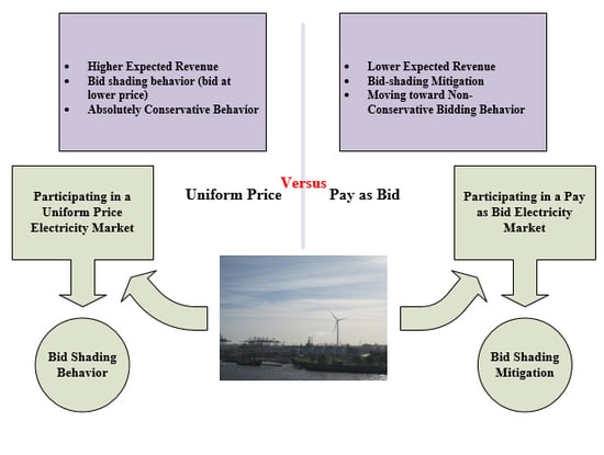
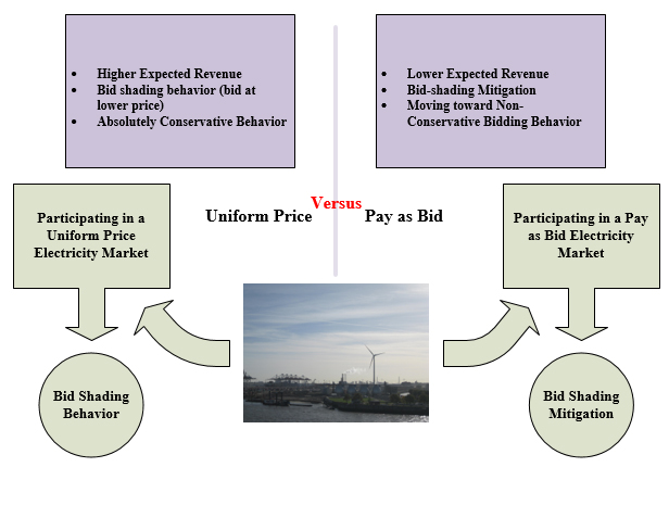
Low variable cost power plants such as wind farms who participate in real Uniform Price (UP) markets exhibit bid shading behavior [5]. Wind farm owners’ bids are conservative. In fact, their bidding behavior is not based on their true long run marginal cost; instead, they shade their bids far below the forecasted market price. Indeed, zero bidding behavior has been observed in UP markets [6]. Investments on the wind farm projects and conventional power plants are also affected by the electricity prices [7]. Although, in a fully competitive UP market, the difference of market clearing price and the marginal cost of participants covers the cost of generation and also makes profit, zero bidding policy of a great portion of market capacity will decrease the overall market price. In the case of high wind penetration, this phenomenon potentially lowers the investment incentives in not only wind power projects but also in other power generation projects as well.

This bidding behavior could be different in a PAB auction such as IEM. Currently, the output power of wind farms is purchased at a fixed tariff. The purchasing price is about 10 times higher than the pre-defined market cap price. Legislated electricity market laws imply a future (long term program), in which the current feed in tariffs policy will be omitted. As a result, wind farm owners will participate in the auction as free agents. From this perspective, it is necessary to analyze the long term bidding behavior of wind farms and their reactions to the market mechanism.

1.2. Problem Statement

A wind farm, as an economic agent, participates in the electricity market to make profit [8]. In order to maximize its profit, it adopts bidding strategies. Since wind speed forecasting techniques are not flawless, wind farms owner should deal with imbalance costs due to deviations from the quantities offered in the auction. The effects of these deviations should be minimized using proper bidding strategies. Zhang et al. [9] used a Markov probability model to obtain the optimum quantity to be sold in the market. The method demonstrates a reduction in the imbalance costs. Matevosyan et al. [10] proposed a stochastic programming approach to solve this problem. The forecasting and probabilistic methods are aggregated in Pinson’s et al. [11] works to minimize the deviation costs. This is inherently a short term problem and it should also be solved in a short run scope.

The major propositions of a bidding strategy are one, the amount of energy offered and two, the bidding price; both in an accurate time schedule. The bidding strategy gives us a micro insight into the policy of an agent for participating in an energy auction. The bidding strategy is not the subject of this paper.

Although bidding strategies are mostly treated as short term optimization problems, long term bidding behavior of agents should also be taken into account. Here the objective is not to generate a time dependent schedule for bidding; instead, the concern is about how an agent would react to an auction mechanism. Our findings should help investors to make wiser decisions when investing in wind farms. It should be noted that our findings will not give a micro insight since the output of a bidding behavior study will not be a set of time dependent prices and quantities to be offered in an auction.

1.3. Literature Review

Two major auction mechanisms are used in electricity markets, namely Uniform Pricing (UP) and discriminatory pricing or PAB [12]. It is widely accepted that in a UP competitive auction, the agents bid their true marginal costs. Bidding the true cost is a long term policy and could be interpreted as a bidding behavior. On the other hand, in a PAB auction, the agents try to forecast the cost of marginal generator and adjust their bids according to this forecast [13]. This is also a bidding behavior. Ren et al. [14] showed that in a PAB mechanism, the optimal behavior is to bid based on a combination of market price uncertainty limits and the true cost. They analytically discuss that both PAB and UP mechanisms leads to similar expected revenues.

However, it is proven that in the electricity markets, contrary to the result of the revenue equivalence theorem, a PAB auction yields less total revenue than a UP auction [15]. Son et al. [15], acknowledged that the long run implications are important. Their focus was on the effect of short term strategic bidding. It should be noted that the discussions advanced by Morey et al. and Ren et al. [12,14], did not cover the uncertainty of generation units such as wind farms. This is the issue that is addressed in this paper having a long run scope.

Most Electricity markets such as Nord Pool, utilize an auction with uniform pricing mechanism (UP) in which all of the winners (producer side) are remunerated based on the market clearing price [16]. In a fully competitive UP market, the market players’ optimal strategy is to bid their marginal cost [17]. Thus, marginal generator defines the market price. However, this inference may not be true in an electricity market with PAB mechanism and requires reconsiderations [17]. Market clearing mechanism could distort the market players biding behaviors and the outcome of the auction. Many controversial issues have been studied in the literatures comparing the features and outcomes of PAB and UP mechanism. UP and PAB markets were subjected to comparing studies with different scopes. The main issues fall into the following categories.

(1)

Electricity market policy makers’ interested issues:

• Which market clearing mechanism is more attractive for a new market player? In a UP market, a player should compare its own marginal cost of generation with the market clearing price whereas in a PAB market, market price is not available to the players. Thus, making a decision about entering into a UP market is easier for a novice player [18].
• Studying the market players’ behaviors: bidding strategies have substantial differences in a UP and PAB market. Bidding based on the short run marginal cost is an individually rational behavior in a competitive UP market but this may not be true in a PAB market [19].

(2)

Market operator interested issues:

• Exercising the market power in UP and PAB mechanism: it is possible for a player to exercise the market power in PAB and UP markets but there is not a consensus about the vulnerability of the market players against the market power within a UP and PAB market. Østergaard [20] introduced some indices to study the market power in the electricity markets.
• The price signals: market clearing price is a useful signal for the market players in a UP market comparing to the average price which is available to the market players in a PAB market.
• In the electricity market, it is desirable to call the generation units which have economic competence (generation units with lower cost of generation). It is reported that in a PAB market this goal may not be achieved [17].

(3)

Market players’ interested issues:

• A UP market imposes higher risks to the market players (producers and consumers) comparing to a PAB market.
• Covering the long run marginal cost of the producers depends on the bidding quantities of the marginal generator in a UP market.
• There is no consensus about the superiority of a PAB or a UP market on maximizing the social welfare.
• There is no consensus about the superiority of the producers’ expected revenue in a PAB or a UP market [21].

In IEM, some reasons convince the policy makers to choose PAB auction mechanism. One of them is the electricity price. In a UP market, all the winners are remunerated by the market clearing price. In IEM, some generators locate in the critical areas and they bid with the cap price in most of the times. Due to the system configuration they win the auction with that price. If UP mechanism has been utilized, these generators become the marginal producer and the market clearing price will be equal to the cap price all the times. For the sake of preserving the competitiveness of the market, a regulated cap price is defined considering the cost of electricity generation by different technologies. The cap price is announced on a yearly basis by Iran Electricity Market Regulatory Board. This provides a competitive environment for the market players to participate in a day ahead wholesale electricity market. Moreover, it makes control over the revenue of the generators which locate in the critical areas. Another aspect is the market monitoring issues. Letting the players to participate in a PAB market requires less effort to monitor the bidding behavior of the market players in IEM. Many factors determine the marginal price of the generators. For instance, the maintenance costs. Due to the political issues, sometimes it is difficult to procure the required auxiliary pieces directly from the manufacturer. This condition could also longer the maintenance period which deprives the generator from the economic opportunities in the market. This may affect the maintenance cost of the generators and could increase the marginal cost of generation. In fact, in a PAB auction there is no concern about comparing the bidding price with the marginal cost of generation which could be an ambiguous parameter due to the political situations of Iran.

It will be shown that in a UP auction, the bidding behavior of a wind farm is not based on the marginal cost of generation. In IEM, PAB mechanism is utilized to clear the electricity market. In a PAB auction participants do not bid equal to the expected market price. Similar phenomena have been reported for bidding the energy portion of PAB reserve market in which the bids are not equal to the expected market price [22]. It is also presented that PAB and UP mechanism lead to different expected revenue for the wind farm owner. This conclusion approves the result of [15] about the non-applicability of revenue equivalence theorem in electricity markets.

1.4. An Introduction to IEM

IEM has three main building blocks namely, the day ahead wholesale market, power exchange and bilateral contracts. The day ahead market is a single sided auction which is hold for the producers. Iran Grid Management Company (IGMC, Tehran, Iran) buys the demand on behalf of the consumers. The producers submit the bidding quantities until 10:00 a.m. the day before the delivery of power and the market is cleared based on the PAB mechanism in 2:00 p.m. Then the players receive the market results.

A security constraint unit commitment is solved every day by IGMC to derive the market results and the players receive the generation schedule for 24 h of the day of the power delivery (operation day). Steam power plants (23%), gas turbines (38%), combined cycle power plants (23%), hydropower plants (14%), and nuclear and renewable energies (2%) constitute the generation mix in IEM. Market clearing price is derived in an hourly basis. All of the producers which offer at a lower price than the market clearing price win the auction but they will be paid based on their bidding price. It may be some difference between the electricity market resulted generation schedule and what is implemented by the system operator (or the market players) in the operation day. It may change the effective prices that are applied to the bills of the market players. For instance, if a forced outage occurs for a player that won the auction (an imbalance caused by a player), it will be subjected to the penalties. On the other hand, another player should provide the power to preserve the system security. It should be noted that ancillary services are not provided using a market based approach in the IEM. The player that procures the power shortage will be remunerated based on the bidding prices submitted in the wholesale electricity market and this may increase the average electricity price. It should be noted that IEM pays attention to the internal constraint of the market players. For instance, if the minimum down time constraint of a generation unit causes a player to win the auction, it will be remunerated based on its average variable cost of generation. In this condition, there are also some generation units that could win the auction if the mentioned minimum down time constraint is relaxed. They will be paid proportional to the difference of their bidding price and their average variable cost. In fact, this difference implies the profit that could be earned by those generation units.

Some constraint may impose limitation to the players in the operation day. For instance, a sudden outage of a transmission line could limit the economic opportunities of the producers (an imbalance causes to network congestion). In this condition, the transmission system owners should pay the penalty of deprived economic opportunity to the producers. This payment is proportional to the difference of the bidding prices and the average variable cost of the generation of the producers. Moreover, it should bear the cost of generation units that should increase their output power (if necessary) based on their bidding prices.

1.5. Approach

Considering the effect of uncertainty of bidding admission on the wind farms expected revenue is the key in developing a method for analyzing long term bidding behavior. The proposed method results in the same bidding behavior that is observed in real UP markets. Given this true signal, the bidding behavior of wind farms in a PAB market is obtained using the proposed method, by assuming that the supporting policies will be omitted and the wind farm owner will become a normal market player.

In the literature, market price and wind speed are considered as uncertainty factors in estimating wind farm long term revenues [23,24,25]. Baringo et al. [25] considered the demand variability and wind power production as the sources of uncertainty. Output power estimation is challenging due to variable nature of wind resources. One could use wind speed forecasting methods for this purpose. However, it has been shown that these methods lead to unacceptable errors in long term studies.

Stochastic models for market price, capital cost and wind farm annual output power based on probability distribution functions are developed [23]. Wind speed patterns cannot be considered using only probability distribution functions, although this is a property of certain wind regimes [26,27]. Gomez-Quiles et al. [24] proposed an econometric approach to quantify uncertainties due to limited data on market price and wind resources, in annual revenue estimation of a wind farm.

In this paper, a stochastic model is used that takes wind speed patterns into consideration. This model is further used to estimate wind farm output power. It should be noted that this method is a special method which is usually applied to long term estimations in order to perform adequacy assessment of wind farm integrated power systems [27,28,29,30,31]. Indeed, this is a common problem in adequacy assessment studies and it is the subject of this paper.

Apart from the uncertainty imposed by market price itself, the admission of wind farm bids in the market is also a source of uncertainty. Participation of wind farms in the electricity markets causes the prices to be decreased [32]. In a UP auction, wind farms show zero bidding behavior [33] and the mentioned uncertainty is nullified unless the market price takes a negative value. The real problem arises when wind farms participate in a PAB auction such as Iran day ahead electricity market. Here, zero bidding will not be an option anymore, since, in a PAB auction, the wind farm owner will be paid his own offered price. Thus, in addition to the uncertainty of market price, the bidding admission uncertainty should also be considered.

In order to consider the bidding admission uncertainty, it is necessary to establish a stochastic model for the market price data. A stochastic market price model is used which is established based on the historical market price data.

Wind farms bidding behavior is categorized into conservative and non-conservative groups. Two indices, namely Expected Price Shortage Period, $EPSP$ and the deviation index, $d$ are introduced. These indices are obtained by combining wind farm and market price stochastic models. Using these indices, a multi-objective optimization problem is established and solved using Genetic Algorithm (GA). The answer demonstrates bidding behavior of the wind farm owners who participate in a PAB market, having considered the uncertainty in bidding admission.

1.6. Paper Organization

This paper is organized as follows. Section 2 explains the stochastic models. Section 3 obtains the introduced indices. In Section 4, the proposed method for considering the uncertainty of bidding admission in obtaining the expected revenue of the wind farms is explained. The concepts of conservative and non-conservative behavior are subsequently introduced. A case study is presented in Section 5. Finally, the conclusions are made in Section 6.

2. Stochastic Models

2.1. Motivation

The accuracy of the forecasted wind speed data varies inversely with respect to length of the prediction period [34]. In a long term period such as a year, accurate forecasting is a complex task.

A long term model of wind speed is perfectly obtainable using probabilistic methods. In fact, long term wind speed data are required to obtain a histogram which is in turn used to develop a stochastic model. Billinton et al. [29] proposed a probabilistic modeling approach for wind farm output power which is widely applied in adequacy assessment studies [27,30]. The same method is used in this paper. In addition to the wind speed histogram, the wind speed pattern is also included in the model.

The output of the mentioned method is illustrated in

Table 1. Wind farm output power stochastic model.

Power (MW)	Probability	${\mathit{T}}_{+}$	${\mathit{T}}_{-}$	Frequency	Bidding Price $\mathsf{\Theta }$
$C_1$	$P_1$	$T_{+1}$	$T_{-1}$	$F_1$	$B_1$
$C_2$	$P_2$	$T_{+2}$	$T_{-2}$	$F_2$	$B_2$
⁞	⁞	⁞	⁞	⁞	⁞
$C_n$	$P_n$	$T_{+n}$	$T_{-n}$	$F_n$	$B_n$

, which consists of $n$ discrete states for wind farm output power $C_i$, corresponding probabilities $P_i$ and frequencies of occurrence $F_i$. One column is added to the proposed model which contains the bidding price for the corresponding row of the output power table. $T_{+i}$ and $T_{-i}$ show the probabilities of transitions to upper and lower states, respectively. The next step is to establish the market price stochastic model. The symbol $\mathsf{\Theta }$ refers to a monetary unit.

2.2. Market Price Model

This is not the first time that the market price is modeled using a stochastic process. Many factors that affect market price have a stochastic nature; for instance, the outage of generation units and the strategic behavior of the market players are both essentially random. Some researchers have regarded the amount of money that consumers spend on their electricity consumption as a random variable [35,36]. In order to consider the uncertainty of bidding admission in the long term expected revenue of a wind farm, it is necessary to establish a stochastic market price model. Long term price data are used to establish the stochastic model. If the whole span between minimum and maximum market price data is divided to $j$ price spans, each span has its own minimum ${\pi }_{j_{\min }}$ ($\mathsf{\Theta }$) and maximum ${\pi }_{j_{\max }}$ ($\mathsf{\Theta }$). Then:

$$\begin{array}{l}{\pi }_{j_{\min }}\le {\pi }_{h\left(t\right)}\le {\pi }_{j_{\max }}\Rightarrow {\pi }_{h\left(t\right)}\in {\pi }_j\\ {\pi }_j=\left(1/m_j\right){\displaystyle \sum _{t=1}^m{\pi }_{h\left(t\right)}},{\pi }_{h\left(t\right)}\in {\pi }_j\\ j=1,2,\mathrm{...},k\end{array}$$

(1)

where $h\left(t\right)$ refers to tth hour of the study time interval and $m_j$ is the number of hours that the price data are in a certain price span. The average of ${\pi }_{h\left(t\right)}$ values in a price span is considered as a price level for that span. The model consists of $j$ price levels. If $n\left({\pi }_j\right)$ indicates the observed number of hours that the price level takes a value from jth price span, the probability of occurrence for that price level can be computed using Equation (2).

$$\overline{P_j}=n\left({\pi }_j\right)/D$$

(2)

where $D$ is the study time interval. If $r_{ij}$ is the number of observed transitions between the considered price levels, the probabilities of transitions are obtained using Equation (3).

$${\overline{T}}_{+ji}=r_{ji}/n\left({\pi }_j\right)$$

(3)

For a certain price level, the probability of transition to upper and lower levels are defined as ${\overline{T}}_{+j}$ and ${\overline{T}}_{-j}$, respectively:

$$\begin{array}{l}{\overline{T}}_{+j}={\displaystyle \sum _{i=1,i>j}^k{\overline{T}}_{+ji}}\\ {\overline{T}}_{-j}={\displaystyle \sum _{i=1,i<j}^k{\overline{T}}_{-ji}}\end{array}$$

(4)

The specifications of the proposed model will be described in the Section 5. Thus far, the wind farm and market price stochastic models have been derived. In the next section, the indices that describe the uncertainty of bidding admission are derived by combining these stochastic models.

3. Indices Describing the Uncertainties

Wind farm and market price stochastic models should be combined in a way that would produce results which can be rightfully interpreted as uncertainty in bidding admission. The first step is to establish the price deviation table using Equations (5) and (6). This table contains $n\times j$ rows and five columns: price deviation level ${\tilde{M}}_i$, probability of occurrence for each level ${\tilde{P}}_i$, probability of transition to higher and lower levels ${\tilde{T}}_{+i}$, ${\tilde{T}}_{-i}$ and finally the frequency of occurrence ${\tilde{F}}_i$. Price deviation level is the difference between the wind farm owner bidding price for the output power level and the market price. The probability of transition to the upper level of price deviation is equal to the sum of the probabilities of transitions to the lower market and higher bidding prices. This upper level corresponds to a higher price deviation value. The opposite is also true for transition to lower levels. ${\tilde{P}}_i$ and ${\tilde{F}}_i$ can be computed using Equations (5) and (6), respectively.

$${\tilde{P}}_i={\overline{P}}_j\times P_n$$

(5)

$${\tilde{F}}_i={\overline{P}}_i\times \left({\tilde{T}}_{+i}+{\tilde{T}}_{-i}\right)$$

(6)

${\tilde{M}}_i$ of some rows of the price deviation table can be the same. These identical rows should be aggregated using Equations (7)–(9). It should be noted that subscript $i$ refers to the identical price deviation levels.

$${\tilde{P}}_a={\displaystyle \sum _{i=1}^h{\tilde{P}}_i}$$

(7)

$${\tilde{F}}_a={\displaystyle \sum _{i=1}^h{\tilde{F}}_i}$$

(8)

$${\overline{T}}_{a,+i}=\left({\displaystyle \sum _{i=1}^h{\tilde{P}}_i\times {\tilde{T}}_{+i}}\right)/{\tilde{P}}_a$$

(9)

$${\overline{T}}_{a,-i}=\left({\displaystyle \sum _{i=1}^h{\tilde{P}}_i\times {\tilde{T}}_{-i}}\right)/{\tilde{P}}_a$$

To obtain the $EPSP$, it is necessary to establish the cumulative price deviation table. This table contains the cumulative probability and frequency for corresponding price deviation levels. For our purpose, the table should be sorted in an ascending order based on the value of ${\tilde{M}}_i$. Starting from the smallest ${\tilde{M}}_i$, the cumulative price deviation table can be obtained using Equations (10) and (11). The subscript $i$ refers to the price deviation table rows.

$${{\tilde{P}}_{cum}}^{\left(i+1\right)}={\tilde{P}}^{\left(i+1\right)}+{{\tilde{P}}_{cum}}^{\left(i\right)}$$

(10)

$${\tilde{F}}_{cum}={{\tilde{F}}_{cum}}^{\left(i+1\right)}+{\tilde{P}}^{\left(i+1\right)}\times \left({\tilde{T}}_{+\left(i+1\right)}+{\tilde{T}}_{-\left(i+1\right)}\right),i\ge 2$$

(11)

The probability and frequency of the first negative ${\tilde{M}}_i$ in the cumulative price deviation table, namely ${\tilde{P}}_{FN}$ and ${\tilde{F}}_{FN}$, provide price shortage expected period and price shortage expected frequency, respectively:

$$EPSP=D\times {\tilde{P}}_{FN}$$

(12)

$$EPSF=D\times {\tilde{F}}_{FN}$$

(13)

In fact, $EPSP$ (h/D) refers to the expected number of hours in the total period of study ($D=8760$ h) during which the bidding prices are lower than the market price. This situation guaranties bidding admission and it is referred by “price shortage”. $EPSF$ (occurrence/D) indicates the number of times during $D$ that the price shortage occurs. Finally, the expected price shortage duration refers to the expected length of price shortage period divided by its occurrence, and it can be obtained using Equation (14).

$$EPSD=EPSP/EPSF$$

(14)

The deviation index is $d$ and it can be obtained using Equation (15).

$$d={\displaystyle \sum _{i=1}^m{\tilde{M}}_i^2}$$

(15)

In fact, this index measures the deviation of the considered price for output power levels from the market price levels. It is clear that the deviation of the considered price from the market price leads to higher values for $d$.

4. Interpreting the Indices

$EPSP$ enables us to have a quantitative description for the value of bidding admission uncertainty. Higher values of $EPSP$ indicate that the expected period in which price shortage will occur is longer and vice versa. The greater the value of $EPSP$ is, the lower the uncertainty in bidding admission would be. As is mentioned before, if the wind farm is considered a price taker player in a UP market, assigning zero values to $B_{n}s$ would be the best policy.

It has been shown that bidding the short run marginal cost in a completely competitive market maximizes the profit in the short run and thus, is the optimum bidding behavior [12]. Taking derivative of the cost function in order to obtain the marginal cost, leads to elimination of fixed costs. For ordinary generation units participating in a UP market, the difference between market clearing price and the bidding price could cover the fixed costs. However, wind farms have large fixed costs. In fact, in comparison with ordinary generation units; wind farm owners are more concerned about bidding admission. This concern has led wind farm owners towards bid shading even in a UP market. Obviously, zero bids will certainly be admitted in the market unless the market price takes a negative value which is a rarity.

However, in a PAB market, if the wind farm owner in order to increase $EPSP$, lowers $B_{n}s$, a problem will arise: lowering $B_{n}s$ could potentially lead to loss of some revenue for the wind farm owner. Having considered the uncertainty of bidding admission, there are two types of possible long term behavior for a wind farm owner. First is to accept low $B_{n}s$ and gain the desired $EPSP$ in order to have a lower bidding admission uncertainty in a PAB market, for the probable cost of reducing the revenue. This is the behavior of a conservative generation company. The second type of company bears the risk of a lower $EPSP$ in return for higher $B_{n}s$ and probably higher revenue. Non-conservative wind farm owners prefer this latter type.

Investigating these contrary long term policies motivated the authors to propose a new method that could model the observed behavior of the wind farm owners in a UP market. The proposed method is subsequently used to model the wind farm behavior in a PAB mechanism.

Thorough investigation of this issue is carried out by establishing a multi-objective optimization problem with two contradictory objectives corresponding to conservative and non-conservative types of behavior. The normalized objective function is defined in Equation (16).

$$OF=-{\mathsf{\omega }}_1\left(d^{-1}/{d^{-1}}_{\max }\right)-{\mathsf{\omega }}_2\left(EPSP/EPS{P}_{\max }\right)$$

(16)

where $d$ and $EPSP$ are dependent on $B_{n}s$ through the value of ${\tilde{M}}_i$. It is obvious that $d$ is directly a function of ${\tilde{M}}_i$ by Equation (15). $EPSP$ depends on the first negative row of the price deviation table. In fact ${\tilde{M}}_i$ values determine this negative row. The $B_{n}s$ are limited to the maximum of ${\pi }_j$ and zero. Considering $B_{n}s$ as the decision variables, the optimization problem is to minimize the weighted sum of the normalized objective function. A nonlinear bounded optimization problem is encountered and Genetic Algorithm is utilized to achieve the solution. $d_{\max }$ and $EPS{P}_{\max }$ should be derived before proceeding with the solution. Note that ${\mathsf{\omega }}_1$ and ${\mathsf{\omega }}_2$ are weighting factors which correspond to the preference of the wind farm owner to be a conservative or non-conservative generation company.

If ${\mathsf{\omega }}_1$ is assigned a greater value with respect to ${\mathsf{\omega }}_2$, emphasis will be on the minimization of deviation index. During the optimization $B_{n}s$ approach higher values that are closer to the market price. The resulting $B_{n}s$ in turn reduce $EPSP$. This is consistent with our intuition, since as $B_{n}s$ get closer to the market price, the uncertainty for bidding admission increases. This is the behavior of a conservative generation company, which is due to the uncertainty of the market price itself.

When ${\mathsf{\omega }}_2$ is assigned a greater value than ${\mathsf{\omega }}_1$, the aim of the optimization is to maximize $EPSP$. In other words, during the optimization process $B_{n}s$ decrease with respect to the market prices and this policy decreases the uncertainty of bidding admission. Considering the above, which type of behavior is more profitable for the wind farm owner? To answer this question, first the expected revenue of the wind farm is calculated by using Equation (17):

$$R_{EXP\_PAB}=D\times {\displaystyle \sum _{i=1}^m{\tilde{P}}_i\times C_i\times B_i}$$

(17)

where $R_{EXP\_PAB}$ refers to the expected revenue of the wind farm in a PAB market. $C_i$ and $B_i$ indicate the output power level and the corresponding price, respectively. Subscript $i$ refers to the rows with positive ${\tilde{M}}_i$, where the price shortage occurs. For a UP market, $B_i$ is replaced with ${\pi }_i$ in Equation (17) to obtain the expected revenue.

The cost of generated energy by the wind farm is comprehensively described using the concept of Levelized Cost of Energy (LCOE). Tegen et al. [37] developed a method that enables the user to calculate the LCOE for the wind farm under study by comparing its specification with a reference wind farm project. The cost of energy produced by the wind farm can be computed using Equations (18) and (19).

$$E=D\times {\displaystyle \sum _{i=1}^n{P}_i\times C_i}$$

(18)

$$C_t=E\times LCOE$$

(19)

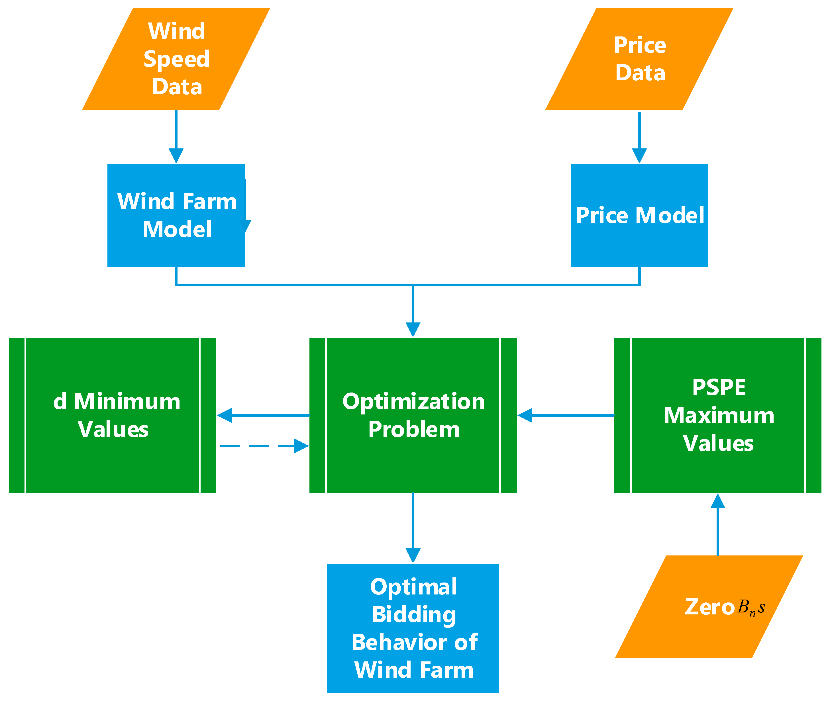
where $E$ refers to the expected energy that will be generated by the wind farm during the period of study and $C_t$ indicates the total cost. The profit earned could be obtained simply by subtracting the cost from the expected revenue. Figure 1 illustrates different steps in obtaining the expected revenue of the wind farm considering the bidding admission uncertainty. The aforementioned relations are all depicted in this figure.

5. Case Study and Discussion

The case study was conducted in Khaf, a border region in the east of Iran where the annual average wind speed is more than 10 (m/s). A wind farm with a nominal capacity of 18-MW was studied. The wind farm included six 3-MW Vestas wind turbines. The stochastic model of this wind farm is illustrated in

Table 2. Eighteen-megawatt wind farm output power stochastic model.

Power (MW)	Probability	${\mathit{T}}_{+}$	${\mathit{T}}_{-}$	Frequency
0	0.2491	0.1068	0	0.0266
3	0.1112	0.2379	0.2104	0.0499
6	0.0397	0.2514	0.2124	0.0184
9	0.0964	0.2335	0.2154	0.0433
12	0.0584	0.1895	0.1810	0.0216
15	0.1983	0.1203	0.1563	0.0548
18	0.2468	0	0.1045	0.0258

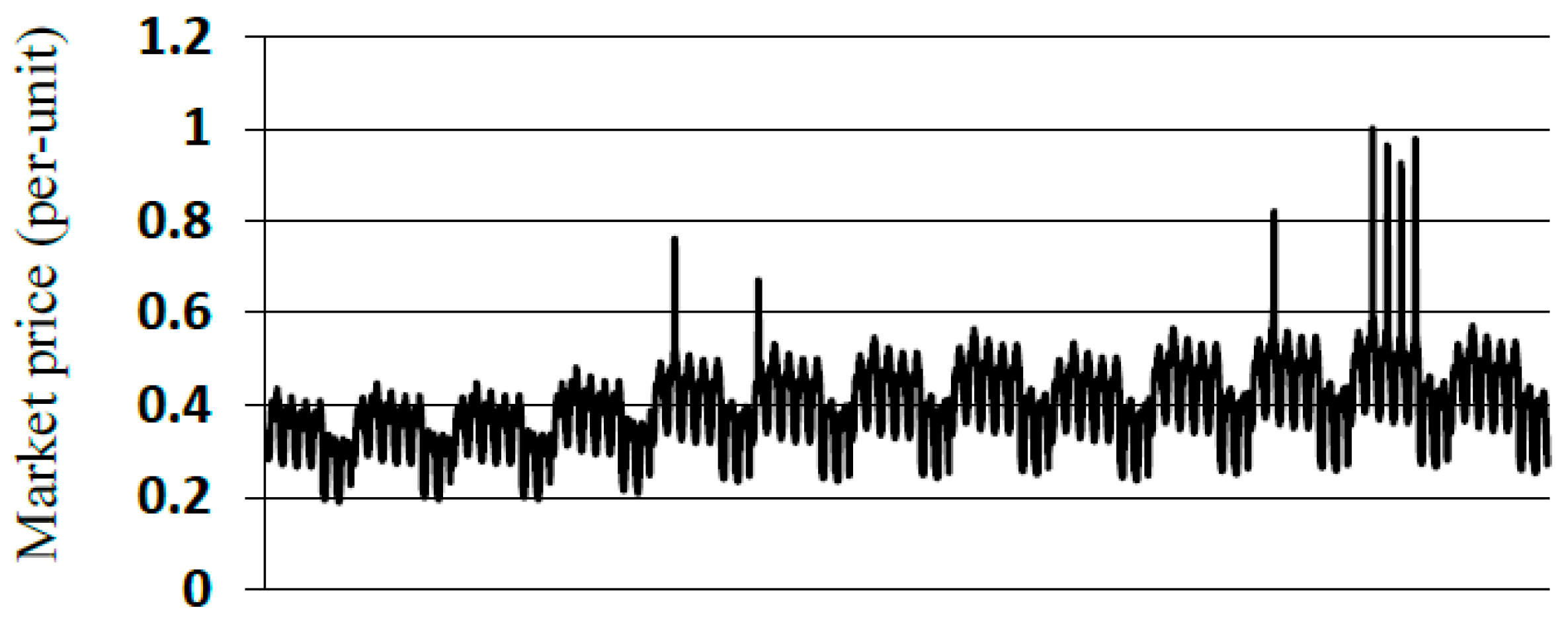
based on the method proposed in [29] and the real wind speed data of the region. Summer market price in the region is also illustrated in Figure 2. Prices are illustrated in per-unit, since authors are not authorized to disclose exact values of the market price. The base is the maximum market price in Figure 2. It is mentioned that in order to consider the uncertainty of bidding admission in the market, a stochastic model should be established for the market price. It will be considered that some discrete states as market price levels and establish the stochastic model based on the proposed method. For the sake of clarity, only a portion of them is illustrated in

Table 3. Market price stochastic model.

Price (Per-Unit)	Probability	$\mathit{T}{\mathit{P}}_{\mathit{w},+}$	$\mathit{T}{\mathit{P}}_{\mathit{w},-}$	Frequency
1	0.0001	0	1	0.0001
0.86	0.01	0.1149	0.6782	0.0079
0.76	0.0495	0.2454	0.3773	0.0308
0.66	0.0719	0.2850	0.4252	0.0511
0.56	0.0593	0.3494	0.4035	0.0446
0.46	0.0375	0.3994	0.2591	0.0247
0.36	0.0169	0.4054	0.2095	0.0104

.

According to the results of the proposed model, in high price levels such as 1 (per-unit), the market price has a great tendency to reduce, considering the probability of transition to lower states. In power markets, the peak price occurs mostly due to the events which are unanticipated by the system operator. For instance, congestion in transmission lines or an abrupt failure in an important generation unit could be considered as events. As soon as the event occurs, suppression measures will be taken by the system operator to mitigate the effects of that event on the power system operation and eventually the market price will decrease to normal levels. The advantage of the proposed model for the market price is that it considers the probability of transition between price levels.

As said before, in addition to the market price uncertainty, the bidding admission uncertainty also affects the expected revenue of wind. The proposed model gives the wind farm owner a quantitative description for this behavior of market price. It does so by considering the probability of transitions between different expected market price levels. The expectations of the wind farm owner regarding the market price levels are also described by the probabilities of occurrences.

Having obtained wind farm and market price stochastic models, $EPSP$, $EPSF$, $EPSD$ and the deviation index can be computed by establishing the cumulative price deviation table. MATLAB^® Optimization Toolbox (R 2015, Energy Technology Department, Aalborg, Denmark, 2015) is used to solve the aforementioned optimization problem.

Depending on the values given to the weighting factors, the wind farm owner is advised to be conservative or not. Different values were assigned to weighting factors in order to investigate the behavior of the introduced indices. It should be noted that these factors describe the aforementioned polices for the wind farm owner. $EPS{P}_{\max }$ is obtained by setting all $B_{n}s$ equal to zero and deriving ${d^{-1}}_{\max }$ by means of solving a primary minimizing problem. It is obvious in Figure 3 that decreasing the value of ${\mathsf{\omega }}_1$ from 1 to 0 (or increasing ${\mathsf{\omega }}_2$ from 0 to 1) will increase the value of $EPSP$. This signifies that the uncertainty of bidding admission is reduced when the policy of the wind farm owner is leaning towards that of a conservative generation company. It is illustrated in Figure 4 how $B_{n}s$ change while the wind farm owner policy approaches a conservative behavior.

It is remarkable that when a wind farm exhibits an absolutely conservative behavior, $B_{n}s$ will be equal to the lower limit of market price. As said before, it is reasonable to say that in order to increase $EPSP$, $B_{n}s$ should be reduced. This will cause the deviation index to increase. Figure 3 confirms these assumptions.

This illustrates that all ${\tilde{M}}_i$s of the cumulative price deviation table take negative values except the one with zero value. In other words, when the bidding behavior is absolutely conservative (${\mathsf{\omega }}_1=0,{\mathsf{\omega }}_2=1$), regardless of the value $B_{n}s$ take between zero and the minimum expected market price, $EPSP$ takes its maximum value. As a result, the value of fitness function remains constant. When the conservative behavior is adopted, the independency of $EPSP$ from values of $B_{n}s$ could be interpreted as adopting zero bidding policy by the wind farm owner. If wind farms have a high penetration factor in the generation portfolio of a market, zero bidding behavior could have some disadvantages. This behavior could lower market price in the short term and as a result, reduce incentive to invest in generation units. Thus it will have undesirable effects in the long term. Therefore, it is not recommended that the market rules force wind farms to participate in a PAB market as a normal market player.

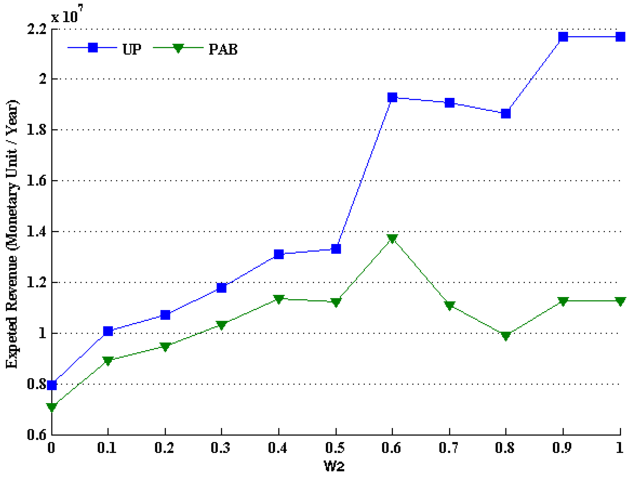
Figure 5 illustrates the expected revenue of the 18-MW wind farm in Khaf which is under investigation for installation. Considering the results, some points are worthy of note: (1) The expected revenue in UP market increases when the wind farm adopted policy is leaning towards conservatism. The maximum expected revenue in a UP market is achieved by adopting an absolutely conservative behavior. As discussed above, this policy corresponds to zero bidding behavior. This behavior has been observed and is addressed in the literature as a typical behavior for a wind farm participating in a UP market. This fact could verify the results of the proposed method; (2) The optimal policy in a PAB market occurs when ${\mathsf{\omega }}_1$ and ${\mathsf{\omega }}_2$ take the values 0.4 and 0.6, respectively.

This issue is clarified by comparing Figure 3 and Figure 6. For a price taker wind farm that cannot manipulate the market price with its strategic policies, the expected revenue in a UP market is higher than a PAB market. In other words, if the wind farm cannot affect UP market conditions with its generation or adopted strategies, it would be better off being a conservative generation company.

Figure 6 illustrates the behavior of the normalized objective function with respect to the weighting factors. The objective function has two extrema where it takes the value of −1. The left side extermum is where the deviation index is minimized and the right extermum is the point in which the $EPSP$ is maximized. It is mentioned that, for wind farm owners, these extrema correspond to non-conservative and conservative types of behavior, respectively. Moreover, extermum point indicates the optimum policy for the wind farm owner, where ${\mathsf{\omega }}_1$ and ${\mathsf{\omega }}_2$ take the value of 0.4 and 0.6, respectively.

This situation indicates that the wind farm owner in a PAB market should adopt a complex policy of 40% non-conservative and 60% conservative behavior. It is predictable that the wind farm owner will choose a behavior between the defined extrema. If a generation company (GENCO) decides to be an absolutely conservative generation company, it should adopt zero bidding behavior, which is not desirable in a PAB market. On the other hand, if GENCO decides to be an absolutely non-conservative generation company, it should completely neglect its concerns about bidding admission. This is consistent with our intuition that a wind farm should choose a moderate policy between conservatism and non-conservatism in a PAB market.

Note that in different markets or for different wind farms, the results could be different. What is of importance is that such description of wind farm strategies could be a clue into describing the market as game in which players, i.e., wind farms, compete in order to reach higher payoffs.

Although, in a PAB market, zero bidding behavior will not be observed, this auction mechanism is not as attractive as a UP auction for wind farm owners. Comparing the expected revenue for these mechanisms, further reveals this fact. Using (20) the expected annual energy generated by the wind farm is equal to 83,730 MWh. If $LCOE$ equals 149.3 ($\mathsf{\Theta }$/MWh), the $C_t$ will stand at $1.2501\times {10}^7$ ($\mathsf{\Theta }$). Considering the results illustrated in Figure 5, the wind farm investor profit will be 1,238,000 and 103,317,000 ($\mathsf{\Theta }$) for PAB and UP market, respectively.

The inherent nature of a UP market is that all of the winners will be remunerated based on the market clearing price. Considering the results, if a wind farm selects a fully conservative strategy (zero bidding policy), it has the opportunity to make benefit in the market. Although the wind farm changes its policy to being less conservative in a PAB market, due to the concerns of bidding admission, it reduces its revenue by bidding lower prices. Thus, as the results confirm a wind farm earns less profit in a PAB market.

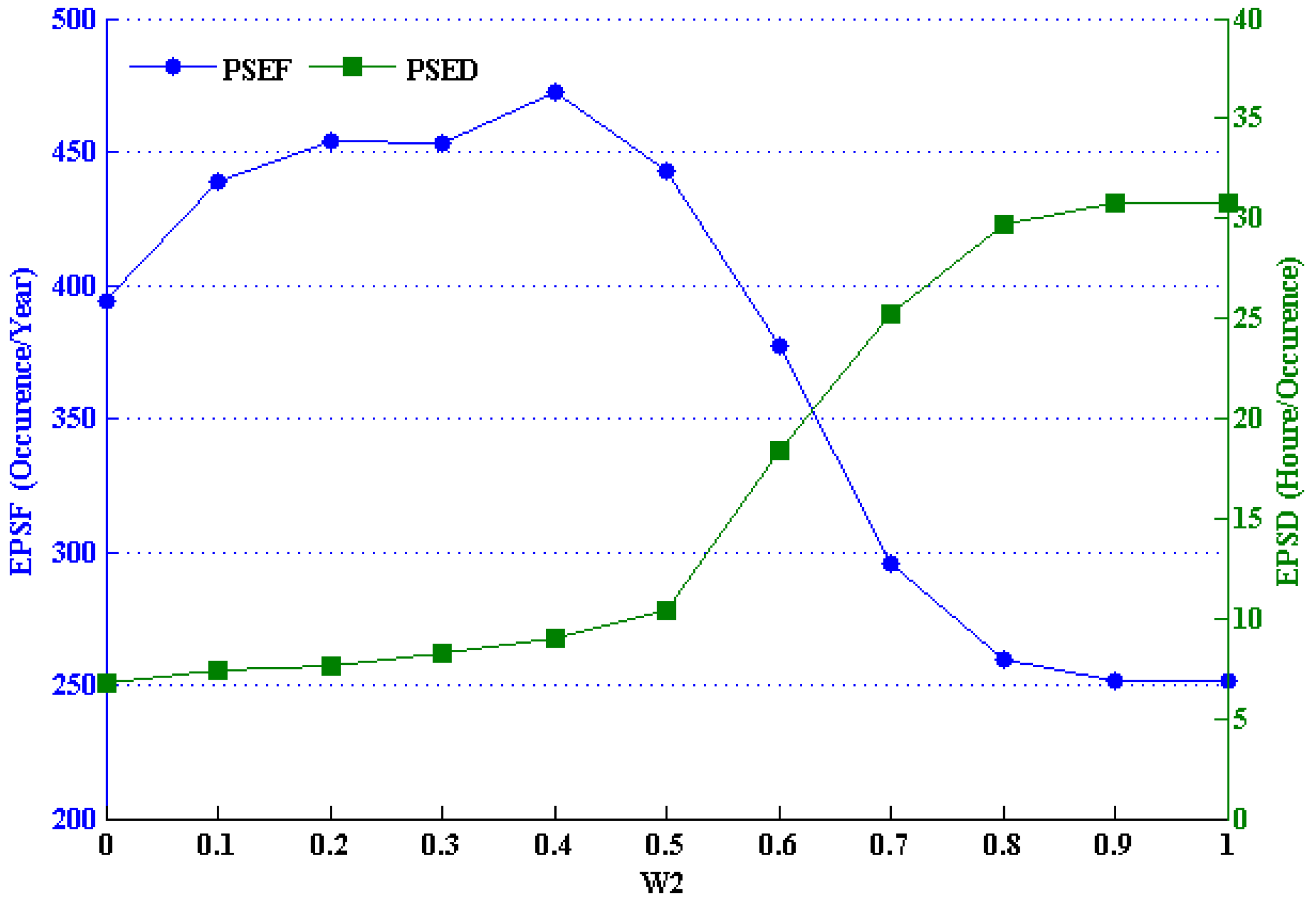
Figure 7 gives a different perspective on the problem. As mentioned earlier, $EPSF$ indicates the number of times that price shortage occurs, i.e., the situation that guaranties bidding admission. On the other hand, $EPSD$ indicates the expected duration of price shortage per occurrence. It may also be a challenge for the wind farm owner to decide whether to consider $B_{n}s$ in such a way that maximizes $EPSF$, $EPSD$ or a combination of both.

As seen in Figure 7, and also by considering results of Figure 5, none of the maximums or minimums represented in the $EPSF$ and $EPSD$ profiles is an optimum point.

In spite of the fact that the proposed method has been used to model long term bidding behavior of a wind farm, it is possible to apply it to short term periods as well; for example, in determining the bidding strategy for an existing wind farm in a day ahead market. For this purpose, the parameter $D$ would be equal to 24 instead of 8760 but applicability and accuracy of the method for short term studies still needs further investigation. It is worthy of note that, for determining the short term bidding strategy, the imbalance costs that are imposed due to deviation from the offered quantity in the auction should also be taken into account.

6. Conclusions

A method was proposed to consider the uncertainty of bidding admission in the long term estimation of expected revenue for wind farms. The long term bidding behavior of a wind farm was classified into two types, namely, conservative and non-conservative. It has been shown that in real UP markets, the optimum policy of a wind farm is to be an absolutely conservative generation company. The result of the proposed model completely conforms to the reported observation in the real UP markets. It shows that the proposed method can be perfectly applied to model this behavior in a UP market because, based on the results, a wind farm prefers to be an absolutely conservative generation company. It means that the owner reduces the bids as much as possible (down to zero) to increase the chance of being a winner in the auction. As a result, it will be remunerated based on the market clearing price and makes profit. If the penetration of the wind farms increase the market price will be reduced because a notable share of the generation system bid with low (or zero) price. The market price reduction is frequently reported in the UP markets with high penetration of the wind farms. This is a warning to the market policy makers because reduction of the market price could reduce the incentives for investing on the generation system and the system security could be affected in the long term.

Moreover, it is shown that, in a PAB market, a complex policy of conservative and non-conservative behavior types should be adopted by the wind farm. As is shown for the case study of this paper, by changing the clearing mechanism from UP to PAB, the wind farm moves from an absolutely conservative generation company to a company which is 40% non-conservative and 60% conservative. This means that in the whole period of study (namely a year) the wind farm will not bid at zero price for 40% of the market hours. Based on the results, although the wind farms move toward a non-conservative behavior in a PAB market, their total expected revenue is reduced. On the one hand, PAB could mitigate the consequences of wind farm bid shading behavior due to this movement. In fact, in a PAB market this is not reasonable for a wind farm to choose zero bidding policy. On the other hand, the revenue reduction occurred in a PAB market could reduce the incentives for investing on the wind farm projects.

It is argued that, contrary to the results of the revenue equivalence theorem, the expected revenue of a wind farm is higher in a UP market in comparison with a PAB market. Thus, it is not recommended to integrate wind farms in a PAB market as normal market players. Electricity market policy makers can apply these results to the study of long term reaction of wind farm owners to market mechanisms. In addition, it could be used to provide consultation to investors who are eager to invest in wind farms.