1. Introduction
There is a growing literature on the provision of “useful exergy” within society and its relationship with economic activity. National “exergy accounting” studies have two primary advantages when accounting for energy use at the societal level. First, exergy is a measure of the capacity of an energy flow to perform physical work and hence may better represent the economic value of energy flows than measures that do not adjust for energy quality [
1]. Second, the energy–economy literature commonly focuses on the “primary” or “final” stages of energy consumption [
2,
3,
4,
5], and therefore fails to capture the significant losses in subsequent conversion stages, as well as the improvements in energy efficiency over time. Exergy accounting attempts to estimate the size and dynamics of exergy flows along the conversion chain, including the magnitude and location of these losses. Hence, national exergy accounting allows for the estimation of the “useful exergy consumption” of a national economy.
National exergy accounting involves estimating the total useful exergy consumption within a national economy over a given period of time, broken down into different categories of end-use, such as lighting and space heating. There have been many iterations of the procedure by which useful exergy outputs are estimated, and important differences remain between different studies [
6]. We explore the importance of these methodological differences by constructing a national exergy account of the United Kingdom for the period 1960–2012, updating the method for allocating the final exergy of industrial heat to end-uses. We then quantify the effect of the different methodological choices on the aggregate results, including estimates of total useful exergy consumption and national exergy efficiency. This leads to suggestions for the most suitable methodology to use, when utilising the useful exergy framework as a basis for examining the relationship between energy and economic growth.
Section 2 introduces important concepts relating to useful exergy and its use in economic analysis, while
Section 3 discusses the exergy accounting methodology, and the approaches adopted for the UK.
Section 4 presents the results of exergy efficiency estimation, while
Section 5 discusses the advantages and disadvantages of each approach.
Section 6 concludes by making recommendations for best practice.
2. Definitions and Concepts
Exergy is formally defined as the maximum physical work that can be extracted from a system as it reversibly comes into equilibrium with a reference environment [
7]. It is a measure of the portion of an energy flow that can be used to perform physical work, i.e., the portion that is “useful”. Exergy is thus a measure of both the quantity and thermodynamic quality of an energy flow. Conceptually, exergy is similar to energy; it is measured in Joules, takes multiple forms (e.g., kinetic, electrical, or chemical), and is converted from one form to another.
The key difference between energy and exergy measures of energy flows arises when considering thermal energy (heat), which is of an intrinsically lower thermodynamic quality. For any given quantity of heat, a temperature-dependent portion constitutes low-grade waste heat that cannot be used to perform physical work; this represents a portion of an exergy flow which has been dissipated, or “destroyed”. Exergy derives from the second law of thermodynamics, which (in one form) states that every transformation process involves the loss of some measure of quality of the system. Energy, on the other hand, is conserved in every transformation process and cannot be destroyed, as per the first law of thermodynamics.
Exergy, like energy, flows through a chain of conversion processes from primary to useful stages, as illustrated in
Figure 1. Primary exergy is embodied within natural resources, and differs from its energy equivalent by a so-called “exergy factor”, which is the ratio of exergy to energy of a given energy carrier (and which for fossil fuels is close to unity). Sources of primary exergy are processed and converted into more readily usable “secondary exergy” forms, such as electricity and refined fuels [
8]. In the example in
Figure 1, the primary energy and exergy content of coal is converted to a secondary form—electricity—with some low-temperature heat wasted.
Final exergy is the secondary exergy delivered to the point of retail for end-use, such as the electrical exergy remaining once all transmission and distribution network losses are accounted for. The last stage of exergy conversion takes place within end-use devices, such as diesel engines and lightbulbs, in which final exergy is converted to a form which is usable in the provision of energy services such as transport, thermal comfort or illumination. This “useful exergy” is the last stage at which it is possible to measure exergy in units such as Joules. At this point it is no longer embodied within an energy carrier, but rather is exchanged for energy services within a “passive system” [
9], such as a building or vehicle. Useful exergy is “held” within a passive system for a period of time whilst providing energy services (heat within a building, momentum in a vehicle), until it is eventually dissipated as low-temperature heat.
Energy efficiency is defined as the ratio of inputs and outputs of a process or system, and is used in different ways, depending on the way in which outputs are defined and measured—these may be in energy terms, physical terms (such as vehicle-kilometres) or economic terms [
10,
11]. “First-law” energy efficiency, η, represents a simple ratio of energy inputs,
Ein, to an associated useful output of energy,
Eout, such as heat or physical work:
This measure is used either to evaluate the performance of individual energy conversion processes, or as a sectoral or national indicator of energy efficiency when energy inputs and outputs are aggregated across sectors or a country. However, there are limitations in using first-law indicators in this way—since heat is not comparable with other, higher quality forms of energy, the measure does not recognise that the same useful output may be achieved with lesser inputs using a different conversion device. For example, for a given amount of thermal energy delivered for space heating, the use of a heat pump over an electrical space heater would require fewer units of electrical energy as an input to obtain the level of output, despite the fact that the latter has a first-law efficiency of nearly 100%. This is illustrated in
Figure 1a,b—whilst there is no energy loss between the final and useful stages, there is significant exergy dissipation as this heat is of a low temperature. Given this, a more accurate reflection of the performance of a conversion process relative to its theoretical maximum is desirable. Such a measure is embodied within “second-law efficiency”, or “exergy efficiency”, ε, which addresses this issue by using the ratio of desired exergy output,
Bout, to exergy input,
Bin:
In using exergy as a metric, the second-law efficiency indicator is bounded between 0 and 100%. This is because the input exergy represents the theoretically maximum obtainable output. Equation (2) can thus also be expressed as:
Given that exergy efficiency provides a measure of system performance relative to a theoretical maximum, exergy lends itself to evaluation of aggregate efficiency trends [
12]. In the emerging field of “exergy economics”, research efforts have sought to use exergy rather than energy measures within the analysis of national economies, often forming a measure of national exergy efficiency.
Whereas a great deal of research has sought to understand the relationship between primary or final energy consumption and economic development [
3,
13,
14] there has been relatively little focus upon either the useful stage of energy provision [
15], or exergy as a measure of “quality-weighted” energy [
1]. As opposed to primary or final energy, it is useful exergy that drives the provision of energy services, the fulfilment of which is one of the fundamental purposes of the economy.
3. National Exergy Accounting Methodology
National exergy accounting studies have evolved from static analyses of a nation’s system of energy provision and consumption [
16,
17,
18], to time series studies focusing on either energy transitions [
19,
20], national energy efficiency [
12], or long-run energy-economy interactions [
21]. It is possible to account for the “embodied” exergy content of any material, and a distinction is made between studies which consider the exergy content of energy carriers alone, and the “extended exergy accounting” method that considers energy alongside wider material resources [
22]. In this paper we focus on the former. The evolution of the methodology for accounting for these energy carriers has been enabled by new datasets on final energy consumption and energy efficiency, as well as developments in the accounting methodology. However, since these developments have not been applied uniformly [
6] successive research findings may not be consistent. There has to date been no attempt to measure the quantitative effect of these different methodological approaches on model results such as national useful exergy consumption. Furthermore, there is scope for improving some aspects of the methodology, including the method of allocating final exergy to heating end-uses (
Table 1) as well as the method of estimating the exergy efficiency of a number of these end-uses.
In this paper we seek to address the above concerns. We construct a useful exergy account of the United Kingdom for the period 1960–2012, and compare the results of useful exergy consumption and national final-to-useful efficiency (i.e., the total quantity of useful exergy consumed within an economy divided by the total amount of final exergy) when approaching different aspects of the methodology in a number of different ways. We pay particular attention to the methods of estimating the exergy efficiency of a number of heat and mechanical drive end-uses. Other methodological aspects examined include the choice of final or primary exergy as the initial boundary of the model, the method of accounting for the primary exergy content of renewable electricity, and the method of allocating the final exergy of industrial heat to end-use categories.
Exergy accounting broadly consists of three steps: (a) converting estimates of primary and/or final energy to exergy equivalents; (b) allocating this data to categories of useful exergy and end-uses; and (c) applying an exergy efficiency to each category to obtain an estimate of useful exergy output. The following sections discuss these stages in further detail as well as the specific steps taken in carrying out this research.
3.1. Accounting for Primary and Final Exergy
To form a national exergy account, data on final and primary energy consumption is first converted to exergy equivalents using well-tabulated “exergy factors”, each specific to a particular energy carrier [
23]. Complete data on national energy consumption are drawn from a variety of national or international statistical bodies. Long-run studies whose initial temporal boundary predate 1960 use disparate sources of energy consumption data such as trade organisations, utility companies” reports and annual government statistics [
19,
20]. For shorter-run accounts, including ours, International Energy Agency (IEA) Energy Balances are currently used [
12,
24,
25,
26], which begin in 1960 for Organisation for Economic Co-operation and Development (OECD) countries and 1971 for non-OECD countries. These consist of complete final and primary energy consumption data, disaggregated by “sectors” (industry, transport, residential, commercial/public services, and agriculture); “subsectors” of industry and transport, e.g., chemicals, paper, road, and rail; and “energy carriers” (see
Supplementary Materials S1 for full list). The Balances provide a consistent basis for allocating final exergy to end-use categories, and for making cross-country comparisons.
A distinction can be made between accounts that are confined to the final and useful stages of exergy provision, and those which also include the primary stage. Due largely to the significant quantity of exergy dissipated in power generation, the choice between these initial boundaries significantly affects measures of national-level exergy efficiency. This is shown in
Figure 2; the difference in UK national exergy efficiency between the two indicators rises from 2.7 to 5.7 percentage points over the period as electricity increases in its share of final exergy.
There are different ways of accounting for the primary energy (and thus exergy) content of renewable electricity [
6,
27,
28], and no consensus on the preferred approach. For electricity from nuclear, the heat generated to produce the electricity tends to be counted as the primary input [
28], making it roughly equivalent to fossil fuel-derived power. Three possible accounting conventions exist for renewables, as follows:
- (1)
Physical content method (PCM): Primary energy (exergy) is defined as the “first energy (exergy) form downstream for which multiple energy uses are practical” [
29]. For renewables, this means counting the energy content of electricity, which is the first form of energy which can be used in multiple ways, as primary energy and exergy. There are some differences between organisations which use the PCM in the method of accounting for solar thermal and geothermal electricity—the IEA use the electricity content times 1/0.33 and 1/0.10, respectively, whilst IPCC Working Group 3 use the energy content of electricity [
27]. In our analysis, we opt to use the latter convention when investigating the PCM.
- (2)
Partial substitution method (PSM): Used by the US Energy Information Administration and British Petroleum (BP), primary exergy is equal to amount of primary exergy which would be required to generate the same amount of final exergy in a fossil fuel power plant [
30]. When investigating the PSM, we use the average efficiency and fuel mix of UK fossil fuel generation in the relevant year to determine this equivalent quantity.
- (3)
Resource content method (RCM): Primary energy is equated to the energy content of the source, as it is found in nature (such as the energy within solar radiation incident upon a solar photovoltaic (PV) panel, or the wind energy incident upon a turbine) [
19]. Primary exergy of renewable electricity is accounted for using a series of technology-specific conversion factors, listed in
Supplementary Materials S2.
3.2. Allocation of Final Exergy to End-Uses
Data on final exergy is allocated to end-uses, each of which exist within a category of useful exergy (
Table 1). Enabled by new allocation techniques developed by Serrenho [
23], the number and disaggregation of end-uses have developed over time. Separate approaches to allocation exist for three classes of energy carrier: combustible fuels (secondary energy carriers derived from fossil fuels and biomass), electricity, and food inputs to draught animal and human muscle work.
The most developed allocation method is based upon the IEA Balances [
23]. For combustible fuels, final exergy data for a given energy carrier within a given sector is allocated to a specific end-use (see
Supplementary Materials S3 for a full allocation list). This is often straightforward, e.g., gasoline use within the “road” subsector of transport. Allocating final exergy to heating end-uses—disaggregated into high, medium and low temperature ranges—is more challenging, particularly in the case of industrial heat. The allocation method previously used a best estimate of heat end-uses in industry sub-sectors [
12,
23]. We improve upon this using an empirically constructed heat map for European industry [
31,
32], which estimates the proportion of final energy for low (<100 °C), medium (100–400 °C) and high (>400 °C) temperature heat in each subsector of industry. We further subdivide the low-temperature category into space heating and water heating (see
Supplementary Materials S4 for detail). As shown in
Figure 3, this has the effect of increasing the relative share of the lower temperature categories in industrial heating final exergy.
Allocating electrical final exergy to end-uses is more challenging. The highest level of electricity disaggregation within the Balances is consumption by subsector, e.g., total domestic use of electricity. This necessitates additional data on the allocation of electricity to end-uses, within each subsector. Since little time series data is available on this, we must resort to extrapolation from the limited available data. Brockway et al. [
12] provide a fairly granular disaggregation of electricity consumption by end-use, and we develop this by including updated data on domestic, commercial and agricultural electricity consumption by end-use [
33,
34,
35]. Detailed information on the allocation method for electrical final exergy is available within the
Supplementary Materials S5.
Food inputs to muscle work are estimated as the total energy content of metabolised food within the manual labour population over a year. The same approach is applied to draught animals. However, since both have provided a negligible contribution to useful exergy in the UK since 1960 they are neglected in what follows.
3.3. Estimating Exergy Efficiencies of End-Uses
Once final exergy has been allocated to end-uses, estimates of useful exergy consumption are obtained by applying an estimate of exergy efficiency to each end-use. The techniques used for estimating exergy efficiencies present one of the greatest sources of uncertainty. Estimates of the efficiency of the high-temperature industrial heat and mechanical drive categories vary widely between different studies [
6], owing to limited data. Since these constitute a significant portion of final exergy use, the results of useful exergy analyses are sensitive to the assumptions used.
In the remainder of
Section 3.3, we describe the methods by which we and previous authors have estimated the efficiencies of end-uses. For the mechanical drive and industrial heating (medium- and high-temperature) end-uses, we use methodological alternatives in order to test the effect of different approaches to efficiency estimation on the resulting estimates of useful exergy and national final-to-useful exergy efficiency. We first define a “base” method for each of these end-uses. We then test alternative methods for each end-use, holding the approach for other end-uses constant on the base method. Based upon the results of these comparisons, we then identify those aspects of the methodology to which overall results are most sensitive.
3.3.1. Mechanical Drive
Early studies [
16,
18,
36,
37] used a single value for the exergy efficiency of each mechanical drive end-use, but values used varied from one study to another. Later studies [
24,
38] first calculated the theoretical maximum efficiency of a gasoline (“Otto cycle”) engine, η
max, as a function of the compression ratio,
r:
They then estimated the efficiency of a real engine by applying a series of “loss factors” (α
i) to account for different types of losses (e.g., frictional, part load):
This “loss factor” method represents the efficiency of the conversion device only: that is, the efficiency of the engine and drive train up to the point of contact between wheels and road. Subsequent losses, through aerodynamic and rolling resistance, are due to the design of the passive system (e.g., aerodynamic profile and weight). Applications of the method incorporate changes in the average compression ratio over time, but hold the loss factors fixed at levels that applied several decades ago [
39]. Moreover, there are issues in extending this method to other types of mechanical drive end-use (e.g., diesel road, aviation and marine), for which data is even more limited. For these end-uses, exergy efficiencies are usually taken from estimates in previous studies, e.g., references [
40,
41].
The second method of estimating vehicle exergy efficiency uses data on the relevant energy service efficiency as a proxy for exergy efficiency. For example, in the case of private cars, a relevant measure of energy service efficiency is vehicle kilometres per litre of fuel. Measures of energy service efficiency incorporate both the conversion device efficiency (e.g., of the engine and drive train) and characteristics of the passive system (e.g., vehicle weight and aerodynamics). Ayres et al. [
40] use an empirical study of US passenger vehicles [
40] to derive a relationship between exergy efficiency, ε, and service efficiency,
x (measured in miles per US gallon), of
for gasoline vehicles. Using US data on drive train conversion efficiency and service efficiency [
42], Brockway et al. [
12] develop this relationship using a best-fit linear exponential function. Using this “proxy method”, one can estimate the exergy efficiency of a mechanical drive end-use given data on its service efficiency, which is more readily available. Estimates can then be made country-specific, accounting for the varying efficiencies of different nations” vehicle fleets. The same authors extend this approach to diesel vehicles, aviation, diesel rail and electric rail. In the absence of sufficient service efficiency data, they applied the exergy efficiency of diesel trains to diesel shipping, and for industrial static motors they used the same exergy efficiency values as in Ayres and Warr [
41] (25%–30% over 1960–2010).
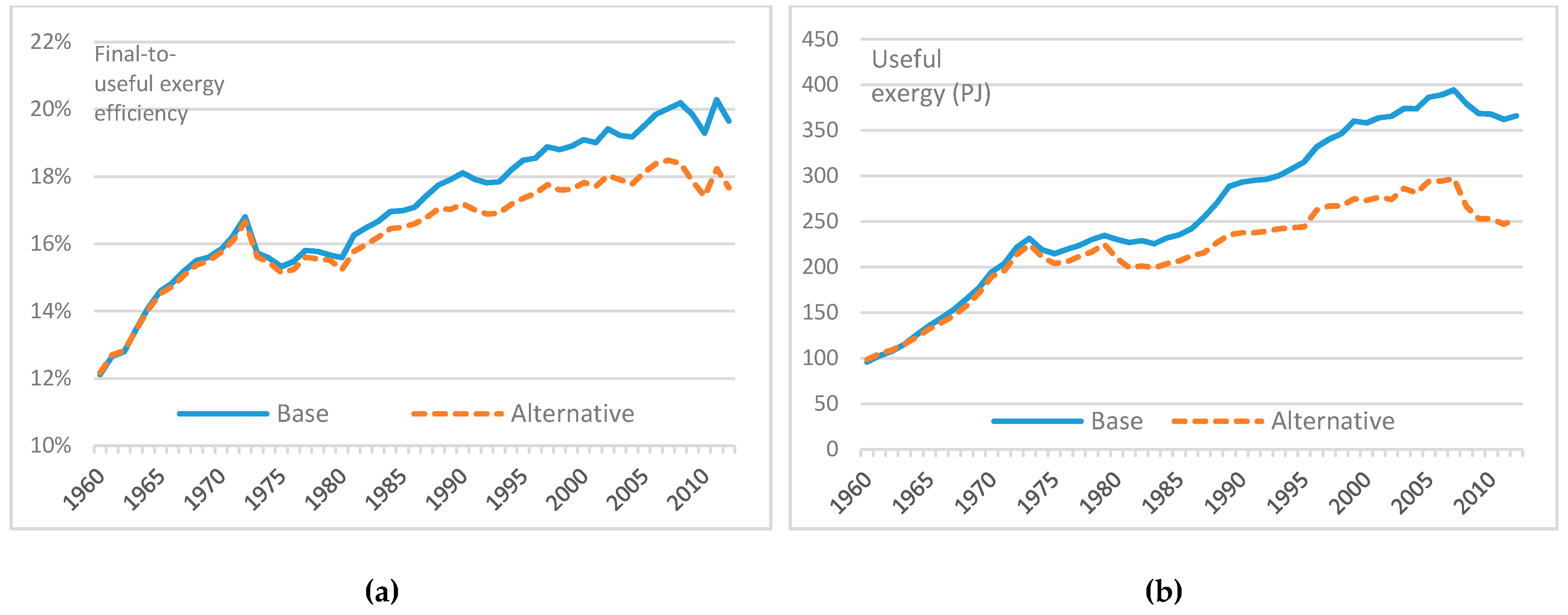
We use two sets of methods to estimate the efficiencies of mechanical drive end-uses. The petrol and diesel road end-uses account for the majority of mechanical drive final exergy (89% in 2012—
Figure 4), and the efficiency of these end-uses in each set corresponds to one of the approaches outlined above, i.e., the “proxy” method for the base method and the “loss factors” approach for the alternative method (
Table 2). Other categories whose efficiencies cannot be estimated with the loss factors/proxy method follow the assumptions of Brockway et al. [
12] and Serrenho et al. [
24] for the base method set and alternative method set, respectively, as detailed in
Table 2.
3.3.2. Heat
The exergy efficiency, ε, of a heating process is related to its corresponding first-law efficiency, η, via a “Carnot factor”,
where
Tc is the temperature of the cold “waste” reservoir and
Th that of the desired process (both measured in Kelvin). Serrenho et al. [
24] use this “Carnot method” to estimate the exergy efficiency of all heating end-uses, whilst Brockway et al. [
12], Ayres et al. [
40] and Ayres and Warr [
41] use it only for low-temperature processes (space and water heating). Each variable on the right-hand side of Equation (6) gives rise to a separate source of uncertainty; these affect the uncertainty in ε differently for different end-uses. For example, for space heating,
Th and
Tc—indoor and outdoor temperatures, respectively—can be estimated with some degree of confidence, given that accurate time series data for both of these variables are available (e.g., time series of average domestic temperature [
43]). Hence, the estimated time series of η is likely to be the primary source of uncertainty in this instance. We return to this point in
Section 4.2.
Within industry heating is used in a wide range of applications and at many different temperatures, and very little data exists on either the temperatures of these applications or of their first-law efficiencies. To address this, Ayres et al. [
40] employ an alternative method of estimating the exergy efficiency of industrial heating which utilises the ratio of the theoretical minimum exergy needed to manufacture a material to the actual exergy consumed in doing so, as defined in Equation (3). There is no clear definition of the theoretical minimum exergy to produce a material: Ayres et al. [
40] use the exergy embodied within rolled steel products, whilst Brockway et al. [
12,
25] use the theoretical minimum energy required to reduce iron ore or melt scrap steel calculated by Freuhan et al. [
44]. These minimum requirements are 8.6 Gigajoules per tonne (GJ/t) of steel produced in a Basic Oxygen Furnace (BOF), and 1.3 GJ/t produced in an Electric Arc Furnace (EAF). Warr et al. [
19] take the same approach but also include some additional exergy for heating iron in a BOF process (10.9 GJ/t in total). Exergy efficiencies are estimated by dividing by these theoretical minima by final exergy consumed per unit of production, using data on the produced mass and energy consumption. Ayres et al. [
40] and Warr et al. [
19] use steel production as a proxy for the exergy efficiency of all high-temperature industrial use of heat in the US; Brockway et al. [
12] use a weighted average of steel and ammonia production in their UK estimate.
We use two methodological alternatives for estimating the efficiency of high- and medium-temperature industrial heat end-uses. For high-temperature industrial heat (HTH), the base method uses the “minimum theoretical exergy/actual exergy” approach, using steel production as a proxy for all HTH applications, with minimum exergy values of 8.6 GJ/t for BOF and 1.3 GJ/t for EAF. The alternative approach uses the “Carnot” method, and within this method we vary the process temperature to reflect the uncertainty in industrial heating temperatures over a large number of processes. We refer to these alternative methods as the “cold Carnot method” and “hot Carnot method”, representing process temperatures of 500 °C and 600 °C, respectively. These temperatures reflect those used for this category by previous authors [
12,
20,
24,
25,
45]. Time series for η is the same as is used by Brockway et al. [
12] and Serrenho et al. [
24], which is adapted from Fouquet [
46].
Medium-temperature industrial heat (MTH) represents drying and evaporation processes driven by steam, in which temperatures range from 100 to 400 °C [
32]. For this end-use, the base method follows the assumptions made by Brockway et al. [
12], whereby the efficiency of this end-use is a function of the HTH efficiency and a ratio of Carnot factors (
Table 3, column 2). This provides methodological consistency between the two industrial heating end-uses, and accounts for the fact that thermodynamically, high-temperature processes are inherently more efficient than those of a lower temperature. The two alternative methods for the MTH end-use are analogous to the cold Carnot and hot Carnot methods for HTH, using 150 °C and 200 °C as process temperatures, respectively, again to reflect the choices of previous authors.
3.3.3. Electricity End-Uses and Renewable Electricity Scenarios
For electrical end-uses in which heat is not a useful output, first-law and exergy efficiencies are equivalent; when useful heat is an output, Equation (6) applies. However, there are difficulties in estimating the efficiency of many electricity end-uses, due to either challenges in defining a first-law efficiency (for example, in computing or consumer electronics), or a lack of efficiency data which is expressed in energy terms. Refrigerator efficiency, for example, is generally expressed with reference to power consumption per unit volume, rather than in useful cooling terms. A full list of electricity end-use efficiency data and sources is available in
Supplementary Materials S4.
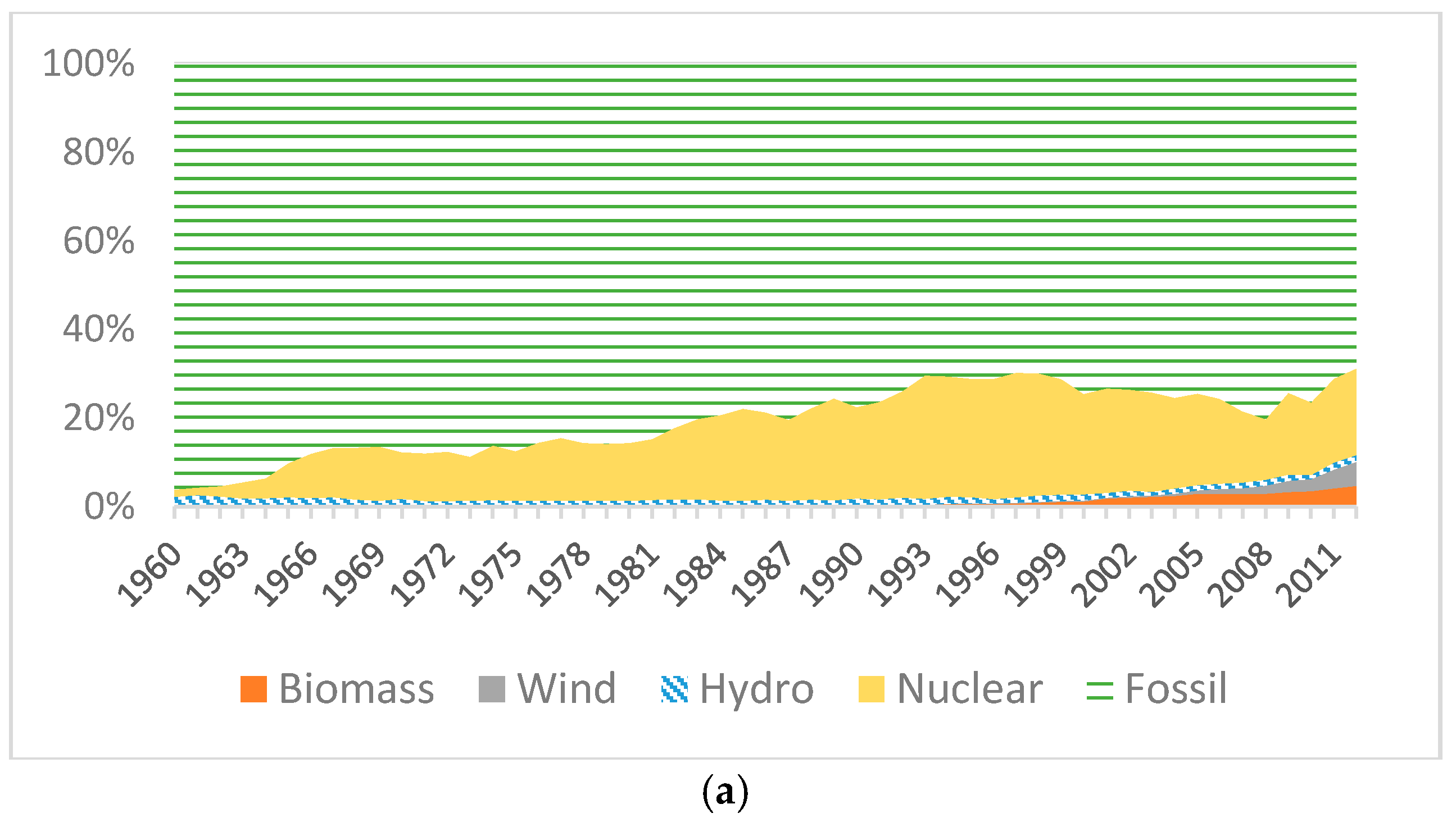
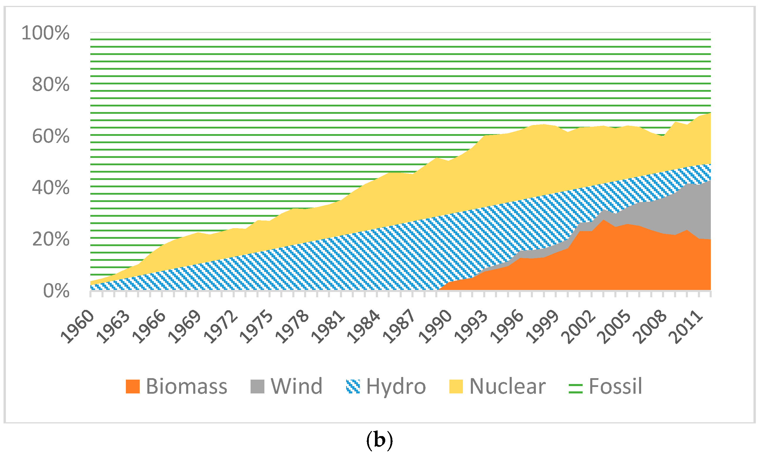
Renewables have to date provided a relatively modest (although growing) share of UK electricity generation—12% in 2012, or 2.6% of final exergy inputs. Hence, the different methods of accounting for primary energy make little difference to historical estimates of useful exergy, but are likely to become more important in the future. To test the sensitivity of our estimates to this variable, we introduce three “high renewables” scenarios to our analysis, in which a significantly larger proportion of historical electricity production was generated using renewables.
Figure 5b illustrates the relative contribution of each technology to electricity production in the high-renewables scenarios, compared to the profile of actual historical production in
Figure 5a. In all three scenarios, the total quantity of electricity produced over the period 1960–2012 is kept at historical values, but the proportion of all renewables in electricity final exergy inputs rises linearly from 2.3% in 1960 to 50% in 2012, with this growth being offset by a proportionately lesser amount of fossil fuel inputs to electricity (nuclear electricity is unchanged). The relative weight of each renewable technology within the total renewable share of final exergy is set equal to historical values. For each of the three scenarios, the primary exergy content of renewable electricity is then estimated using one of the three accounting methods.
5. Discussion
By focusing on the capacity of energy to perform physical work at the useful stage of the energy conversion chain, useful exergy may potentially offer valuable insights into the economic role of energy. This could be explored through econometric analysis of the relationships between useful exergy and economic indicators (e.g., value added or GDP), using techniques that are widely applied to data on primary and final energy consumption—such as Granger causality tests. In order to undertake such analysis rigorously, however, the methodology for estimating useful exergy must be applied consistently. This has not been the case to date.
Constructing useful exergy accounts using country-specific data for a range of economies could provide a richer set of insights into exergy-economy relationships. Most studies to date have focused upon a small number of developed countries such as the UK, US and Portugal [
12,
20,
21]. One of the few exceptions to this is Serrenho et al. [
24], who investigate the EU-15, but the authors resort to using data on either the UK or Portugal to estimate exergy efficiencies for the whole EU. We suggest that the adaptability of a particular methodology to a diverse range of economies is an important criterion for its use in future studies.
There is a relatively constant trend in the range between the minimum and maximum estimates of both national exergy efficiency and total useful exergy consumption shown in
Figure 15. This suggests that on aggregate, the national exergy accounting methodology is fairly robust to the assumptions of the methodology tested in this paper. Whilst some of these assumptions can affect model results such as end-use useful exergy consumption, when taking into account all of the methodological differences the level of variation in results does not significantly change the overall picture of exergy consumption.
We have shown that one of the most significant aspects of the methodology on aggregate levels of useful exergy is the method by which the efficiency of high-temperature industrial heat is estimated. The base method approach (the ratio of theoretical minimum exergy to actual exergy used in selected industries) benefits from well-documented data on iron, steel and ammonia production and energy use. Thus the principle question in using this method is the extent to which these industries are representative of all high-temperature industrial heat processes. The Carnot method provides a higher estimate of exergy efficiency, and is less sensitive to the process temperatures assumed under the cold and hot Carnot methods. Hence the majority of uncertainty under this method may arise from first-law efficiency values. Given the wide range of heat processes employed across different industries and different countries, as well as the lack of data collected on first-law efficiency of these processes, we argue that the ratio of minimum exergy to actual exergy used in selected industries may be more a more suitable measure of exergy efficiency, at least until more disaggregated data on the process temperature and first-law efficiency of industrial processes becomes available. We also suggest that where data availability permits, a broader selection of industries is included under this approach, particularly non-metallic minerals (such as cement and clinker production) and non-ferrous metals (such as aluminium), for both of which heat demand consists largely of high-temperature heat.
The base method of estimating the efficiency of medium-temperature industrial heat (the product of HTH exergy efficiency and a ratio of Carnot factors for medium and high industrial temperatures) is problematic, given that it results in an efficiency which is lower than that of the water heating end-use (see
Supplementary Materials S6)—a result that is thermodynamically inaccurate since higher temperature processes should be more efficient. With this in mind, we suggest that the Carnot method is more appropriate for the MTH category, using a process temperature of 150°C. This seems a reasonable first approximation of low temperature industrial processes, much of which is steam-driven [
40,
47].
There is a general consensus in previous studies on using the Carnot method to estimate the efficiency of space and water heating processes, partly because there is considerably less ambiguity concerning the process and reference temperatures used in these processes. Uncertainty in the first-law efficiency of these processes is therefore the dominant factor in the efficiencies of these end-uses. Data on first-law efficiency must encapsulate the dynamics of a number of different heating technologies, including solid biomass, oil furnaces, and condensing gas boilers, as well as the efficiency of each. Fouquet [
48] provides valuable estimates of first-law efficiency for the UK, though further work is required to collect this data for other countries.
Our analysis of the mechanical drive category has focused upon the end-uses which account for the most final exergy, such as petrol and diesel road vehicles. Previous work has attempted to incorporate devices at an early stage of development such as biofuel or natural gas vehicles [
12,
20], though we suggest that until a) these end-uses account for more final exergy, and b) more data on efficiency is available for these vehicles, then these should be neglected. A potential exception to this is plug-in hybrid and battery-electric vehicles, which may diffuse more rapidly given policy support. Following this suggestion, we consider the method of estimating the efficiency of petrol and diesel road vehicles. The method of using service efficiency as a proxy for exergy efficiency incorporates elements of the passive system design as opposed to the loss factors method which does not. It has been argued previously [
6] that exergy efficiency estimates should be limited to the boundary between conversion device and passive system (i.e., should consider only the drive train), and that a separate layer of analysis should be applied to incorporate the way in which the passive design affects the delivery of an energy service. However, by incorporating service efficiency into the efficiency estimation, a more accurate measure of the utility provided by the energy service is obtained which partly fulfils the role of this additional layer of analysis. Although this does raise an issue of consistency with other mechanical drive end-uses such as industrial static motors, we suggest that the proxy method of measuring road vehicle efficiency is the most robust approach available. This can also incorporate national data on vehicle mileage and energy use more readily, supporting cross-country analysis.
We have demonstrated that in countries in which renewables comprise a significant portion of final electricity production, the method of accounting for primary exergy can have a significant effect upon aggregate primary exergy and hence national primary-to-useful exergy efficiency. The partial substitution method is beneficial in resource accounting, reflecting the amount of fossil fuel generation offset by renewables, but is of little use when analysing the economic value of energy. If the primary exergy of the renewable resource is counted (resource content method), primary to secondary efficiency is particularly low for technologies such as solar PV and wind, which can result in an overall decline in national efficiency when these are deployed at scale. This perception of high exergy dissipation is arguably only of minor concern when considering such technologies, given that the resource is renewable. This issue fundamentally relates to the point along the energy conversion chain at which the boundary of primary exergy is situated. For example, the energy content of fossil fuels is the embodiment of thousands of years of accumulated solar energy, converted with very low efficiency [
49]—the argument could be made to incorporate this into estimates of primary to secondary efficiency. The physical content method (equating the energy content of electricity with primary exergy) largely avoids this issue, though it precludes the ability to incorporate improvements in the efficiency of renewable conversion devices (e.g., improvements in PV panels). In many analyses of useful exergy-economic growth relationships, primary exergy may only be of secondary interest. If the hypothesis is made that useful exergy is an important factor in economic growth, then estimates of primary exergy would only be required in order to compare the strength of its relationship with economic growth relative to that of useful exergy. Further studies could neglect primary exergy entirely. We suggest that if primary exergy is a necessary indicator in economic analysis, then the physical content method is the preferable method when considering renewables.
6. Conclusions
We constructed a national exergy account for the United Kingdom for the period 1960–2012, using IEA Balance data on primary and final energy consumption. We allocated this data to a number of end-uses whilst improving the method for allocating industrial heat, and calculated the exergy efficiency of each end-use in order to estimate national useful exergy consumption and national exergy efficiency. To test the sensitivity of model results to different assumptions used to estimate efficiency, we employed a number of methods for estimating the efficiency of industrial heating and mechanical drive end-uses. We then compared estimates of useful exergy resulting from these against a constant base method. The effect of different methodological choices for accounting for the primary exergy content of renewable electricity was also investigated.
Table 4 summarises the importance of different assumptions for methodological choices and shows suggestions for best practice.
A number of important implications for future research in exergy economics, as well as energy economics more broadly, arise from this research. First, the methodological suggestions made could contribute towards a greater level of consistency across future exergy accounting studies. Given the relatively small amount of research carried out in this area to date, it is important that successive studies are able to reproduce results; doing so with a consistent method of accounting for primary, final and useful exergy will help to strengthen the validity of conclusions. This in turn could allow exergy economics to provide interesting new insights into the relationship between energy and economic growth. The second implication arising from this research is that there remains a need for further improvement in the certain areas of the methodology. In particular, improved time series data for a number of parameters, across different countries, would improve the accuracy of future accounts. Specific areas in which data could be improved includes the service efficiency of diesel road vehicles and trucks (such that the two can be disaggregated), as well as diesel rail, shipping and aviation; first-law efficiency data of industrial and domestic heating devices; and exergy efficiency data for electronic devices. Aside from these areas, we have shown that the overall methodology is fairly robust to different methods of estimating end-use exergy efficiency.


