Robust Unit Commitment Including Frequency Stability Constraints

Abstract

An increased use of variable generation technologies such as wind power and photovoltaic generation can have important effects on system frequency performance during normal operation as well as contingencies. The main reasons are the operational principles and inherent characteristics of these power plants like operation at maximum power point and no inertial response during power system imbalances. This has led to new challenges for Transmission System Operators in terms of ensuring system security during contingencies. In this context, this paper proposes a Robust Unit Commitment including a set of additional frequency stability constraints. To do this, a simplified dynamic model of the initial system frequency response is used in combination with historical frequency nadir data during contingencies. The proposed approach is especially suitable for power systems with cost-based economic dispatch like those in most Latin American countries. The study is done considering the Northern Interconnected System of Chile, a 50-Hz medium size isolated power system. The results obtained were validated by means of dynamic simulations of different system contingencies.

1. Introduction

The increased use of variable generation technologies (VGTs) such as wind power and PV generation has led to new challenges for TSOs, especially from a frequency viewpoint [1,2,3]. The main reasons are the operational principles and inherent characteristics of these technologies, which are essentially different from those of conventional synchronous generators (SGs):

• VGTs usually maximize their power production, i.e., no operating reserves are sustained for frequency control.
• VGTs have changing availability levels over time (variability), which cannot be predicted with perfect accuracy (uncertainty). As the level of VGTs increases, the additional variability and uncertainty introduced in the system will cause an increase in the operating reserves requirements, thus imposing additional regulation burdens on the remaining SGs.
• Unlike conventional SGs, converted-based VGTs have no inertial response unless additional control actions are taken.

The replacement of a large number of SGs by inertia-less VGT units will not only be a detriment to the frequency regulation but also lead to a reduction in the overall inertia of the system. As a consequence, a power system’s ability to arrest frequency deviations during disturbances, and thus its security, may be significantly affected.

The current security practices adopted by TSOs when planning the commitment of their generation units are not sufficient to ensure system security in the case of major power imbalances. These practices are typically based on requiring a predefined amount of operating reserves in order to ensure frequency control [4,5]. The reserve’s quantification is usually done by taking into account the size of the largest possible generation infeed [4,5]. However, this approach does not consider the inertial response of conventional SGs or the dynamic performance of other system components. As a consequence, current security practices used in the Unit Commitment (UC) process may fail in ensuring system stability during major power imbalances, especially in periods with high injections of inertia-less VGTs.

During the last few years, only a few research works have been published in the field of economic dispatch models including system frequency constraints [2,4,5,6]. All these works assume that the scheduling of the generation units is known a priori. The inclusion of frequency restrictions within the framework of the UC has received comparatively less attention. For instance, Ahmadi and Ghasemi [7] proposed a security-constrained unit commitment (SCUC) including additional constraints to represent the system frequency response. To do this, a system frequency response model is derived and then used to find an analytical representation of the frequency nadir of the system. Another SCUC formulation is presented by Restrepo and Galiana [8]. In this work, primary and tertiary reserve constraints are simultaneously taken into account in the optimization process. The set of used constraints is based upon the droop characteristic of the SGs in steady state, thus neglecting the dynamic response of the machines. Daly et al. [9] also proposes a similar work. Another related work is presented by Ela et al. [10]; however, the authors do not focus on the impact of renewables on frequency response, nor deal with any source of uncertainty. Likewise, Chang et al. [11] do not address the uncertainty in renewable generation or how the penetration of renewables impacts on the frequency response of the system; however, the way to characterize frequency response follows the same principle as that presented in our work. In conclusion, although [7,8,9,10,11] present improved UC models when compared to traditional approaches, these models fail to consider the uncertain nature of VGTs. Indeed, the inherent uncertainty of these technologies in the time frame of the one-day-ahead UC makes the results of deterministic UC models less reliable.

This paper proposes a two-stage Robust Unit Commitment (RUC) including a set of additional frequency stability constraints. To do this, a simplified model of the initial system frequency response during contingencies is obtained, starting from the swing equation. This simplified model is then used in combination with historical frequency nadir data during contingencies to obtain the frequency constraints. The constraints included in the RUC ensure that system frequency will not drop below a predefined lower threshold after any single generation contingency. Then, the contribution of this paper is to develop a RUC model able to deal with both wind power uncertainty during normal operation and large power imbalances from a frequency stability standpoint. This is accomplished by introducing the abovementioned constraints into the RUC formulation. As we will show in Section 6, the designed strategy is capable of improving the frequency response of the real-world power system described in Section 5 when considering high levels of VGT penetration.

The scope of the present study is the development of a UC model able to deal with wind power uncertainty during normal operation but also robust during contingencies from a frequency stability standpoint.

2. Forecasting and Scenario Generation

A typical practice to manage the inherent uncertainty when dealing with renewables is to incorporate forecasting errors by means of stochastic modeling techniques [12,13]. Likewise, one can also use rather simple approaches such as fixed intervals [14,15,16]. In this work, the forecasting methodology proposed by Álvarez-Miranda et al. [17] is adopted for predicting the power generation from VGTs in a one-day-ahead UC setting. This forecasting approach yields a model of uncertainty that exploits the main characteristics of both the interval and the scenario representation of the uncertainties: (i) rather narrow intervals are enough to capture the whole range of values defined by the forecasting process; and (ii) a small number of scenarios is enough to assure that most of the possible realizations are enclosed into the calculated scenarios. The methodology is described below.

2.1. VGTs Power Forecast via Bootstrapping

Let $D^{*}$ be the day for which the VGT generation must be forecast on an hourly basis. Assume that there exist resource measurements (such as wind speed or solar radiation) of an interval of time, say a whole month. In order to forecast the levels of VGT of the first $\mathsf{\tau }$ periods (hours) of $D^{*}$, the method produces $\mathcal{P}$ paths (or series) of forecast values (see [17] for details). After the $\mathcal{P}$ paths of these first $\mathsf{\tau }$ hours are obtained, the average value of each hour is calculated using these $\mathcal{P}$ paths, and the resulting values $({\overline{\mathrm{w}}}_1,\dots ,{\overline{\mathrm{w}}}_{\mathsf{\tau }})$ are appended to the real data. Afterwards, the forecasting procedure is performed again in order to obtain $\mathcal{P}$ paths for the following $\mathsf{\tau }$ hours. The process is repeated until the levels of VGT for the whole day (or days) under consideration have been forecasted. The iterative use of the re-sampling procedure developed by Pascual et al. [18] is a key element of the described method.

2.2. Scenario Generation

Once the aforementioned process is finished, a set of scenarios given by series of intervals is calculated. Basically, for each period one associates a discrete set of scenarios, and each scenario is characterized by a series of resource availability intervals (e.g., a wind speed interval for each hour). Moreover, no assumption is made regarding the probability of the occurrence of either of these scenarios or the probability distribution of the values within the intervals.

For each period $t$ of day $D^{*}$, an interval $\left[w_t^{\text{min}},w_t^{\text{max}}\right]$ is calculated by choosing a pair of paths assuring that at least 90% of the forecast values are contained within them. Additionally, we calculate the average forecast value across all paths, ${\overline{w}}_t$. Once this is done, the interval associated with $t$, and corresponding to scenario $\mathsf{\omega }$, is generated by the following two steps: (i) the upper limit $w_t^{\mathsf{\omega }+}$ is randomly (and uniformly) taken between ${\overline{w}}_t$ and $w_t^{\text{max}}$; (ii) the lower limit $w_t^{\mathsf{\omega }-}$ is randomly (and uniformly) taken between $w_t^{\text{min}}$ and ${\overline{w}}_t$. For each given scenario, this procedure is repeated until we have forecast values for the whole day, or series of days, under consideration.

3. Robust UC Formulation

This section summarizes the formulation of the proposed robust UC. It is important to note that this approach is suitable for power systems with cost-based economic dispatch like in most Latin American countries.

3.1. Hedging against VGT Power Fluctuations

The previously described scenario generation approach enables TSOs to plan for a set of scenarios that take into account the inherent uncertainty of VGTs. The next phase is to use a mathematical model to incorporate these scenarios to optimize the UC decision. For such purposes, the strategy proposed by Álvarez-Miranda et al. [17] is used. This modeling tool relies on an extension of the concept of budget of uncertainty originally proposed by Bertsimas and Sim [19]. The main difference is that the model of uncertainty provided in Bertsimas and Sim [19] corresponds to intervals, while the model of uncertainty proposed by Álvarez-Miranda et al. [17] corresponds to a set of scenarios, and each of them associates intervals.

For the sake of simplicity, the remainder of this section considers wind power generation as unique VGT. However, the proposed model can easily be extended to other types of VGT.

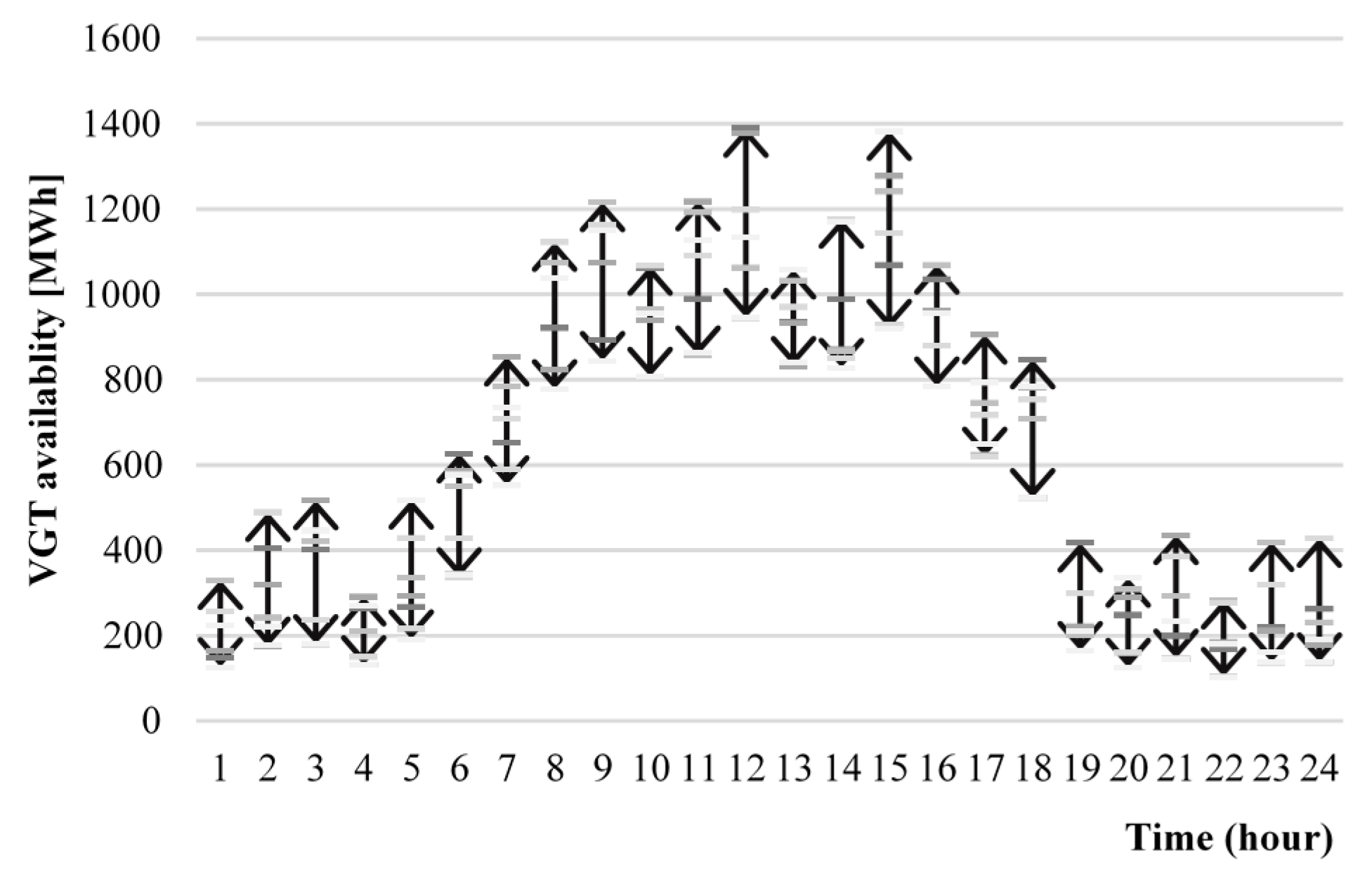
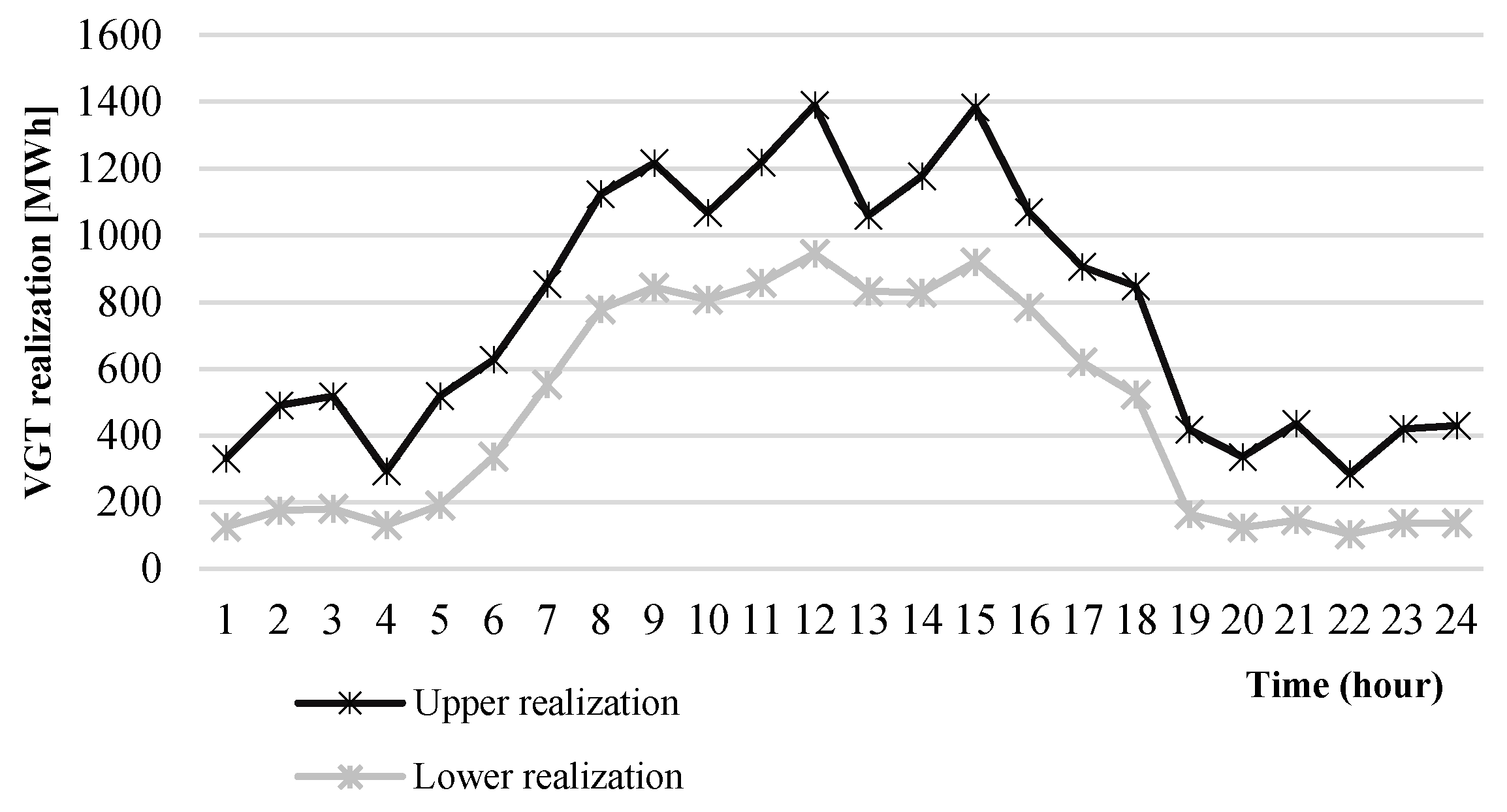
Recall that $D^{*}$ is a generic day (or set of days) divided into $T$ periods. Let $\mathrm{\Omega }$ be a set of scenarios (${\mathsf{\omega }}_1,\dots ,{\mathsf{\omega }}_{\left|\mathrm{\Omega }\right|}$), so that for a given scenario $\mathsf{\omega }\in \mathrm{\Omega }$ and for a given period $t\in \left\{1,\dots ,T\right\}$, there is an interval [$q_t^{\mathsf{\omega }-},q_t^{\mathsf{\omega }+}$] (with midpoint ${\overline{q}}_t^{\mathsf{\omega }}$). From the power generation point of view, an optimistic data realization is such that the actual wind power $q_t$ is $q_t^{\mathsf{\omega }+}$; on the contrary, a pessimistic one is $q_t=q_t^{\mathsf{\omega }-}$.

Suppose that a decision-maker is able to translate her/his level of conservatism against uncertainty through a pair $({\mathrm{\Gamma }}^{+},{\mathrm{\Gamma }}^{-})$; where ${\mathrm{\Gamma }}^{+}$ is the maximum number of periods that the wind-power is at the upper limit, and ${\mathrm{\Gamma }}^{-}$ is the minimum number of periods that the wind-power is at the lower limit. If ${\mathrm{\Gamma }}^{+}={\mathrm{\Gamma }}^{-}=0$, it means that the TSO assumes that the wind-power values at all periods will be at the corresponding midpoints; if ${\mathrm{\Gamma }}^{+}=24$ and ${\mathrm{\Gamma }}^{-}=0$, then $q_t$ can take any value within [$q_t^{\mathsf{\omega }-},q_t^{\mathsf{\omega }+}$]; if ${\mathrm{\Gamma }}^{-}=24$ (and regardless of the value of ${\mathrm{\Gamma }}^{+}$), then wind-power values will be set at the lower bounds. In practice, parameters ${\mathrm{\Gamma }}^{+}$ and ${\mathrm{\Gamma }}^{-}$ allow TSOs to obtain solutions that are protected against scenarios with large fluctuations from the midpoints. This translates into a protection against the uncertainty and variability of wind power. The common setting considers only one parameter $\mathrm{\Gamma }$ (see, e.g., [14,19]), which in this context would correspond to ${\mathrm{\Gamma }}^{+}$. One can see that ${\mathrm{\Gamma }}^{-}$ controls the level of conservatism, while ${\mathrm{\Gamma }}^{+}$ controls the level of optimism.

In addition to the aforementioned notation, let $B$ be the set of buses, and ${\mathrm{\Lambda }}_b$ be the set of generators at bus $b\in B(\mathrm{\Lambda }={\cup }_{b\in B}{\mathrm{\Lambda }}_b)$. Now, let $\mathit{q}\in {ℝ}_{\ge 0}^{\left|B\right|\times \left|\mathrm{\Omega }\right|\times T}$, be a vector of real-valued variables such that $q_{bt}^{\mathsf{\omega }}$ corresponds to the actual wind-power (in $\text{MW}$) injected at bus $b$ in period $t$, if scenario $\mathsf{\omega }$ is realized. For simplicity, let ${\widehat{q}}_{bt}^{\mathsf{\omega }+}=(q_{bt}^{\mathsf{\omega }+}-{\overline{q}}_{bt}^{\mathsf{\omega }})$ and ${\widehat{q}}_{bt}^{\mathsf{\omega }-}=({\overline{q}}_{bt}^{\mathsf{\omega }}-q_{bt}^{\mathsf{\omega }-})$. In addition, the auxiliary variables ${\mathit{z}}^{+}\in {\left\{0,1\right\}}^{\left|B\right|\times \left|\mathrm{\Omega }\right|\times T}$ and ${\mathit{z}}^{-}\in {\left\{0, 1\right\}}^{\left|B\right|\times \left|\mathrm{\Omega }\right|\times T}$ are needed. These variables are such that if $z_{bt}^{\mathsf{\omega }+}=1$ and $z_{bt}^{\mathsf{\omega }-}=0$, then the wind-power injection at bus $b\in B$, at a given period $t\in \left\{1,\dots ,T\right\}$ and for a given scenario $\mathsf{\omega }\in \mathrm{\Omega }$, is at its upper limit $q_{bt}^{\mathsf{\omega }+}$. Likewise, if $z_{bt}^{\mathsf{\omega }+}=0$ and $z_{bt}^{\mathsf{\omega }-}=1$, then the wind-power is at its lower limit $q_{bt}^{\mathsf{\omega }-}$; and if $z_{bt}^{\mathsf{\omega }+}=z_{bt}^{\mathsf{\omega }-}=0$, then the wind-power is at its midpoint ${\overline{q}}_{bt}^{\mathsf{\omega }}$. Variables $\mathit{q}$, ${\mathit{z}}^{+}$ and ${\mathit{z}}^{-}$ are related by the following inequalities:

$$q_{bt}^{\mathsf{\omega }}\le {\overline{q}}_{bt}^{\mathsf{\omega }}+{\widehat{q}}_{bt}^{\mathsf{\omega }+}{z}_{bt}^{\mathsf{\omega }+}-{\widehat{q}}_{bt}^{\mathsf{\omega }-}{z}_{bt}^{\mathsf{\omega }-}, \forall t\in \left\{1,\dots ,T\right\}, \forall b\in B$$

(1)

$${\displaystyle \sum _{t=1}^T}{z}_{bt}^{\mathsf{\omega }+}\le {\mathrm{\Gamma }}^{+} \text{and} {\displaystyle \sum _{t=1}^T}{z}_{bt}^{\mathsf{\omega }-}\ge {\mathrm{\Gamma }}^{-}, \forall b\in B$$

(2)

$$z_{bt}^{\mathsf{\omega }+}+z_{bt}^{\mathsf{\omega }-}\le 1 \forall t\in \left\{1,\dots ,T\right\}, \forall b\in B.$$

(3)

$$({\mathit{z}}^{+},{\mathit{z}}^{-})\in {\left\{0, 1\right\}}^{2\times \left|B\right|\times \left|\mathrm{\Omega }\right|\times T}$$

(4)

Consequently, for a given scenario $\mathsf{\omega }\in \mathrm{\Omega }$, the corresponding uncertainty set is given by:

$${\mathcal{Q}}^{\mathsf{\omega }}({\mathrm{\Gamma }}^{+},{\mathrm{\Gamma }}^{-})=\left\{{\mathit{q}}^{\mathsf{\omega }}\in {ℝ}_{\ge 0}^{\left|B\right|\times T}|(1)-(4)\right\}.$$

(5)

This uncertainty set, which is shaped by the pair $({\mathrm{\Gamma }}^{+},{\mathrm{\Gamma }}^{-})$, is embedded into the mathematical optimization model presented next.

3.2. MILP Formulation for the TSRUC

In the following, the Mixed Integer Linear Programming (MILP) formulation for the two-stage RUC is presented.

3.2.1. Parameters

$S_i^b$ is the start-up cost for generator $i$ at bus $b (\$)$; $S{D}_i^b$ is the shutdown cost for generator $i$ at bus $b (\$)$; $G_i^b$ is the minimum time that generator $i$, at bus $b (\mathrm{h})$, must be operating after it is turned on; $H_i^b$ is the minimum time that generator $i$, at bus $b (\mathrm{h})$, must be down after it is turned off; $R_i^b$ is the ramp-up limit for generator $i$ at bus $b (\text{MW})$; $P_i^b$ is the ramp-down limit for generator $i$ at bus $b (\text{MW})$; $L_i^b$ is the minimal output of electricity if generator $i$ at bus $b$ is on $(\text{MW})$; $U_i^b$ is the maximum output of electricity if generator $i$ at bus $b$ is on $(\text{MW})$; and $D_t$ is the total demand on the system in period $t (\text{MW})$ (including an estimation of the system losses).

3.2.2. First-Stage Variables

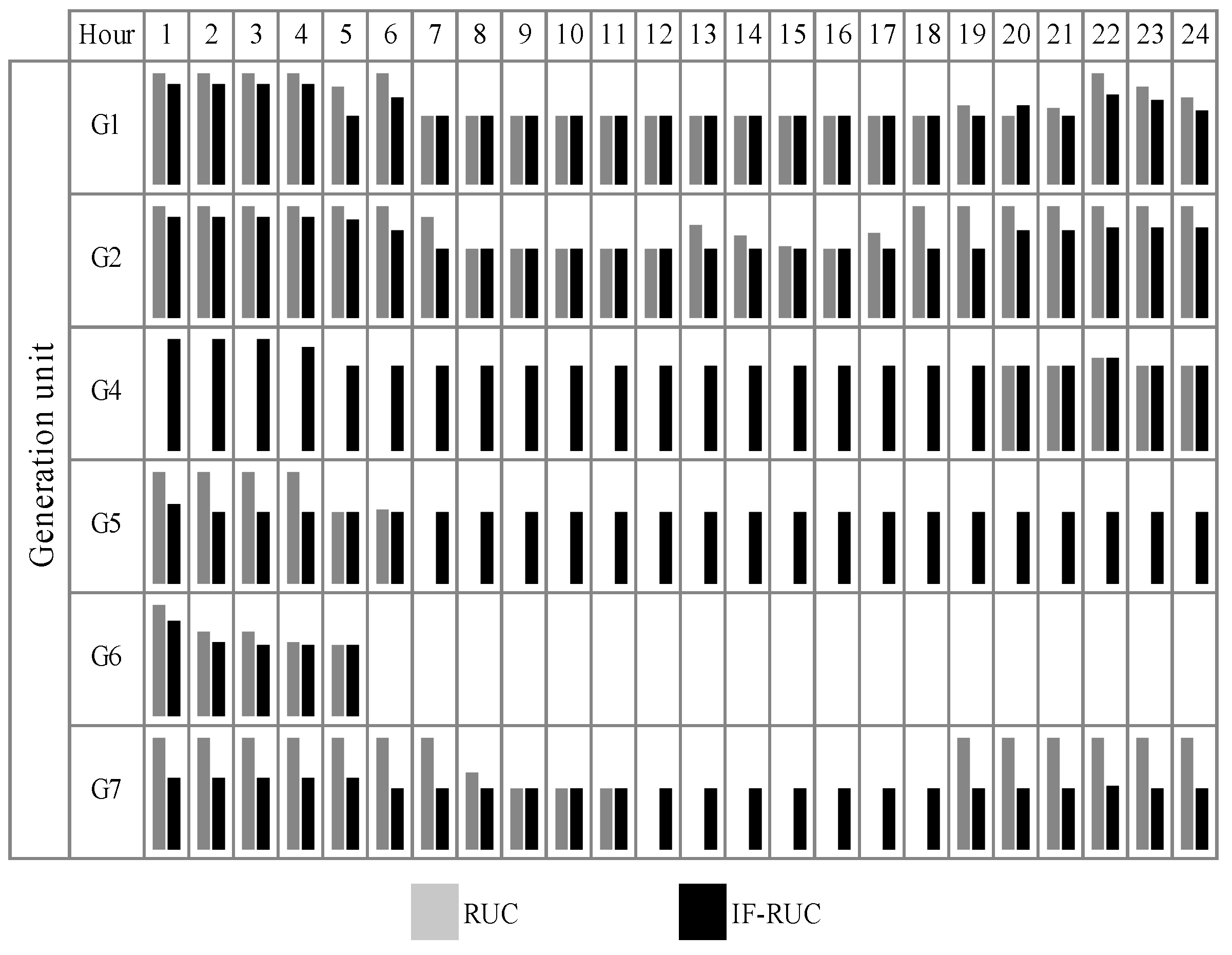
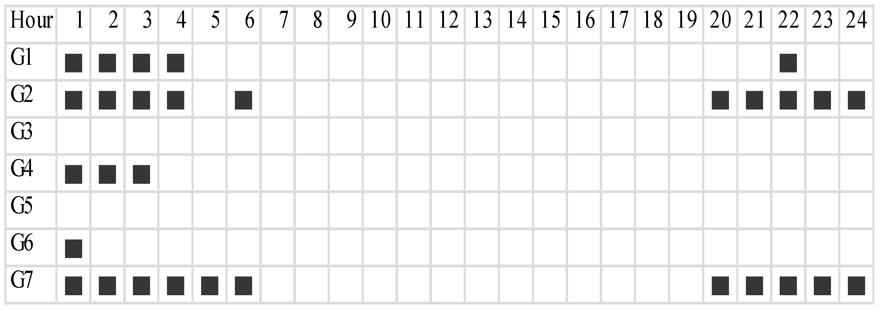
$\mathit{y}\in {\left\{0, 1\right\}}^{\left|B\right|\times \left|\mathrm{\Lambda }\right|\times (T+1)}$, binary variables such that $y_{it}^b=1$ if generator $i$ at bus $b$ is on in period $t$, and $y_{it}^b=0$ otherwise; $\mathit{u}\in {\left\{0, 1\right\}}^{\left|B\right|\times \left|\mathrm{\Lambda }\right|\times T}$, binary variables such that $u_{it}^b=1$ if generator $i$ at bus $b$ is started up in period $t$, and $u_{it}^b=0$ otherwise; $\mathit{v}\in {\left\{0, 1\right\}}^{\left|B\right|\times \left|\mathrm{\Lambda }\right|\times T}$, binary variables such that $v_{it}^b=1$ if thermal generator $i$ at bus $b$ is shut down in period $t$, and $v_{it}^b=0$ otherwise. These first-stage variables allow us to define today which generating units will be operating, and for how long, tomorrow. Note that, for practical purposes, $\mathit{y}$ variables are also defined for $t=0$.

3.2.3. Second-Stage Variables

$\mathit{x}\in {ℝ}_{\ge 0}^{\left|B\right|\times \left|\mathrm{\Lambda }\right|\times \left|\mathrm{\Omega }\right|\times T}$, real-valued variables such that $x_{it}^{b\mathsf{\omega }}$ corresponds to the amount of power generated by generator $i$ at bus $b$ in period $t$, if scenario $\omega$ is realized $(\text{MW})$; $\mathsf{\delta }\in {ℝ}_{\ge 0}^{\left|B\right|\times \left|\mathrm{\Lambda }\right|\times \left|\mathrm{\Omega }\right|\times T}$, real-valued variables such that ${\mathsf{\delta }}_{it}^{b\mathsf{\omega }}$ corresponds to the amount of primary reserve of generator $i$ at bus $b$ in period $t$, if scenario $\mathsf{\omega }$ is realized $(\text{MW})$; and $\mathsf{\mu }\in {ℝ}_{\ge 0}^{\left|B\right|\times \left|\mathrm{\Lambda }\right|\times \left|\mathrm{\Omega }\right|\times T}$ (resp. ${\mathsf{\mu }}^{\prime }\in {ℝ}_{\ge 0}^{\left|B\right|\times \left|\mathrm{\Lambda }\right|\times \left|\mathrm{\Omega }\right|\times T}$), real-valued variables such that ${\mathsf{\mu }}_{it}^{b\mathsf{\omega }}$ (resp. ${{\mathsf{\mu }}^{\prime }}_{it}^{b\mathsf{\omega }}$) corresponds to the amount of positive (resp. negative) secondary reserve sustained by generator $i$ at bus $b$ in period $t$, if scenario $\mathsf{\omega }$ is realized $(\text{MW})$. Second-stage decisions define the so-called dispatching problem, i.e., how much energy will be produced tomorrow by each of the committed units.

The goal of the mathematical optimization setting is to find a cost-efficient one-day-ahead operation policy, i.e., a UC schedule for tomorrow, such that it minimizes a worst-case measure of the operating cost of the second-stage decisions.

Any feasible unit schedule must respect the typical time coupling constraints related to the minimum up and down times of the SGs: (i) if a unit $i$ at bus $b$ is turned on, then it must remain in that state for at least the minimum-up time $(G_i^b)$; (ii) if a unit $i$ at bus $b$ is shut down, then it must remain in that state at least the minimum-down time $(H_i^b)$. These two constraints, plus the nature of the variables, are modeled as follows:

$$-y_{i(t-1)}^b+y_{it}^b-y_{ik}^b\le 0, \forall b\in B, \forall i\in {\mathrm{\Lambda }}_b, \forall t, k\in \left\{t, t+1,\dots ,G_i^b+t-1\right\}$$

(6)

$$y_{i(t-1)}^b-y_{it}^b+y_{ik}^b\le 1, \forall b\in B, \forall i\in {\mathrm{\Lambda }}_b, \forall t, k \in \left\{t, t+1,\dots ,H_i^b+t-1\right\}$$

(7)

$$-y_{i(t-1)}^b+y_{it}^b-u_{it}^b\le 0, \forall i\in {\mathrm{\Lambda }}_b,\forall b\in B, \forall t\in \left\{1,\dots , T\right\}$$

(8)

$$y_{i(t-1)}^b-y_{it}^b-v_{it}^b\le 0, \forall i\in {\mathrm{\Lambda }}_b,\forall b\in B, \forall t\in \left\{1,\dots , T\right\}$$

(9)

$$y_{i0}^b=0, \forall i\in {\mathrm{\Lambda }}_b, \forall b\in B$$

(10)

$$\mathit{y}\in {\left\{0, 1\right\}}^{\left|B\right|\times \left|\mathrm{\Lambda }\right|\times (T+1)}, \mathit{u}\in {\left\{0, 1\right\}}^{\left|B\right|\times \left|\mathrm{\Lambda }\right|\times T} \text{and} \mathit{v}\in {\left\{0, 1\right\}}^{\left|B\right|\times \left|\mathrm{\Lambda }\right|\times T}.$$

(11)

Constraints (6) and (7) model the two operating constraints described above. Constraints (8) and (9) relate variables $y_{it}^b$, $u_{it}^b$ and $v_{it}^b$. Constraint (10) defines the boundary conditions for any feasible unit scheduling and constraint (11) requires that all first-stage variables be binary.

3.2.4. Reserves

Along with Constraints (6)–(11), a conventional cost-based economic UC model includes primary and secondary reserve requirements. Let ${\Delta }_1(\mathit{x},\mathit{y},t)$ be a function indicating the amount of primary reserve required at each period; let $\pi$ be the maximum portion of the nominal capacity of the generators that can be used for primary reserve. Likewise, ${\Delta }_2(\mathit{x},\mathit{y},t)$ (resp. ${{\Delta }^{\prime }}_2(\mathit{x},\mathit{y},t)$) represents the amount of positive (resp. negative) secondary reserve required at each period. The amount of operating reserve at each period depends on the practices of the pertinent TSO and on characteristics of the system. The quantification of the operating reserves is done in order to cope with wind power variability and uncertainty, and also with demand fluctuations. Considering this, the constraints that ensure the operating reserves of the system for a given scenario $\mathsf{\omega }\in \mathrm{\Omega }$ are given by:

$$x_{it}^{b\mathsf{\omega }}+{\mathsf{\delta }}_{it}^{b\mathsf{\omega }}+{\mathsf{\mu }}_{it}^{b\mathsf{\omega }}\le U_i^b{y}_{it}^b, \forall i\in {\mathrm{\Lambda }}_b,\forall b\in B, \forall t\in \left\{1,\dots ,T\right\}$$

(12)

$$x_{it}^{b\mathsf{\omega }}-{{\mathsf{\mu }}^{\prime }}_{it}^{b\mathsf{\omega }}\ge L_i^b{y}_{it}^b, \forall i\in {\mathrm{\Lambda }}_b,\forall b\in B, \forall t\in \left\{1,\dots ,T\right\}$$

(13)

$${\mathsf{\delta }}_{it}^{b\mathsf{\omega }}\le \mathsf{\pi }{U}_i^b{y}_{it}^b, \forall i\in {\mathrm{\Lambda }}_b,\forall b\in B,\forall t\in \left\{1,\dots ,T\right\}$$

(14)

$${\displaystyle \sum _{b=1}^B}{\displaystyle \sum _{i\in {\mathrm{\Lambda }}_b}}{\mathsf{\delta }}_{it}^{b\mathsf{\omega }}\ge {\Delta }_1(\mathit{x},\mathit{y},t), \forall t\in \left\{1,\dots ,T\right\}$$

(15)

$${\displaystyle \sum _{b=1}^B}{\displaystyle \sum _{i\in {\mathrm{\Lambda }}_b}}{\mathsf{\mu }}_{it}^{b\mathsf{\omega }}\ge {\Delta }_2(\mathit{x},\mathit{y},t)+q_{bt}^{\mathsf{\omega }}-q_{bt}^{\mathsf{\omega }-}, \forall t\in \left\{1,\dots ,T\right\}$$

(16)

$${\displaystyle {\sum }_{b=1}^B{\sum }_{i\in {\mathrm{\Lambda }}_b}}{{\mathsf{\mu }}^{\prime }}_{it}^{b\mathsf{\omega }}\ge {{\Delta }^{\prime }}_2(\mathit{x},\mathit{y},t)+q_{bt}^{\mathsf{\omega }+}-q_{bt}^{\mathsf{\omega }}, \forall t\in \left\{1,\dots ,T\right\}.$$

(17)

Constraints (12) and (13) ensure the feasibility of both the dispatched power and operating reserves. Constraints (14) and (15) enforce the primary reserve. Finally, constraints (16) and (17) model the positive and negative secondary reserves, respectively.

3.2.5. Dispatch Problem

Without loss of generality, we will assume that the generation cost of a generator $i\in {\mathrm{\Lambda }}_b$, at bus $b\in B$, in period $t\in \left\{1,\dots ,T\right\}$, and in scenario $\mathsf{\omega }\in \mathrm{\Omega }$, is given by a piecewise linear function $f_i^b : x_{it}^{b\mathsf{\omega }}\to {ℝ}_{\ge 0}$. Thus, for a given feasible scheduling encoded by a collection $(\widehat{\mathit{y}},\widehat{\mathit{u}},\widehat{\mathit{v}})$ satisfying (6)–(11), a pair $({\mathrm{\Gamma }}^{+},{\mathrm{\Gamma }}^{-})$, and a scenario $\mathsf{\omega }\in \mathrm{\Omega }$, the corresponding second-stage dispatching problem is given by:

$$\mathsf{\rho }(\widehat{\mathit{y}},\widehat{\mathit{u}},\widehat{\mathit{v}},\mathsf{\omega })=\text{min}{\displaystyle \sum _{t=1}^T\sum _{b=1}^B\sum _{i\in {\mathrm{\Lambda }}_b}}{f}_i^b(x_{it}^{b\mathsf{\omega }})$$

(18)

$$L_i^b{y}_{it}^b\le x_{it}^{b\mathsf{\omega }}\le U_i^b{y}_{it}^b, \forall t\in \left\{1,\dots ,T\right\}$$

(19)

$$x_{it}^{b\mathsf{\omega }}-x_{i(t-1)}^{b\mathsf{\omega }}\le h_D(y_{i(t-1)}^b,y_{it}^b,L_i^b,R_i^b), \forall t\in \left\{2,\dots ,T\right\}$$

(20)

$$x_{i(t-1)}^{b\mathsf{\omega }}-x_{it}^{b\mathsf{\omega }}\le h_U(y_{i(t-1)}^b,y_{it}^b,L_i^b,P_i^b), \forall t\in \left\{2,\dots ,T\right\}$$

(21)

$${\displaystyle \sum _{b=1}^B}\left({\displaystyle \sum _{i\in {\mathrm{\Lambda }}_d}}{x}_{it}^{b\mathsf{\omega }}+q_{bt}^{\mathsf{\omega }}\right)\ge D_t, \forall t\in \left\{1,\dots ,T\right\}$$

(22)

$$\text{Constraints} (19)–(21) \text{hold} \forall i\in {\mathrm{\Lambda }}_b, \forall b\in B$$

(23)

Constraints (12)–(17)

(24)

$${\mathit{q}}^{\mathsf{\omega }}\in {\mathcal{Q}}^{\mathsf{\omega }}({\mathrm{\Gamma }}^{+},{\mathrm{\Gamma }}^{-}), {\mathit{x}}^{\mathsf{\omega }}\in {ℝ}_{\ge 0}^{\left|B\right|\times \left|\mathrm{\Lambda }\right|\times T} \text{and} {\mathsf{\delta }}^{\mathsf{\omega }}\in {ℝ}_{\ge 0}^{\left|B\right|\times \left|\mathrm{\Lambda }\right|\times T}.$$

(25)

The objective Equation (18) aims to find the minimum cost of the dispatch of the SGs. Constraint (19) ensures that if a generating unit is operative, then it must produce at least $L_i^b$ and at most $U_i^b$. Constraints (20) and (21) correspond to the up and down ramp constraints, respectively. Constraint (22) indicates that the total generated power, including the used wind-power, must satisfy the demand (and the expected losses) in every period. Constraints (23) and (24) ensure the technical correctness of the solution, and constraint (25) characterizes the nature of the second-stage variables. Although transmission constraints are not considered, they could be easily included in the formulation. This was done because the main focus of this work is to include frequency stability constraints in the UC problem.

3.2.6. RUC

For a given first-stage solution $(\widehat{\mathit{y}}, \widehat{\mathit{u}}, \widehat{\mathit{v}})$, the robust dispatching cost $R(\widehat{\mathit{y}}, \widehat{\mathit{u}}, \widehat{\mathit{v}})$ corresponds to the maximum (minimum) dispatching cost among all $\omega \in \mathrm{\Omega }$, i.e.,

$$R(\widehat{\mathit{y}}, \widehat{\mathit{u}}, \widehat{\mathit{v}})\ge {\displaystyle {\sum }_{t=1}^T{\sum }_{b=1}^B{\sum }_{i\in {\mathrm{\Lambda }}_b}}{f}_i^b(x_{it}^{b\mathsf{\omega }}), \forall \mathsf{\omega }\in \mathrm{\Omega }.$$

(26)

Combining the aforementioned constraints and definitions, the RUC is formally defined as:

$$OP{T}_{ℛ}=min{\displaystyle {\sum }_{t=1}^T{\sum }_{b\in B}{\sum }_{i\in {\mathrm{\Lambda }}_b}}(S_i^b{u}_{it}^b+S{D}_i^b{v}_{it}^b)+R(\widehat{\mathit{y}}, \widehat{\mathit{u}}, \widehat{\mathit{v}}).$$

$$\begin{array}{cccccc}\mathrm{s}.\mathrm{t}.& & & & (6)–(17); (19)–(25),& \forall \mathsf{\omega }\in \mathrm{\Omega }, \text{and} (26).\end{array}$$

Regardless of which scenario is actually realized, an optimal first-stage scheduling $(\mathit{y},\mathit{u},\mathit{v})$ can be categorized as robust if it displays the following three characteristics: (i) it is economically efficient (due to the minimization of the worst case); (ii) it is protected against fluctuations of wind-power (which is possible due to the combined effect of $({\mathrm{\Gamma }}^{+},{\mathrm{\Gamma }}^{-})$); and (iii) it is reliable with respect to possible errors in the wind-power forecasting (due to the tailored procedure to generate forecast data).

4. Frequency Stability Constraints

The frequency constraints considered in this work are built on the premise that the rate of change of frequency ($ROCOF$) during the first seconds after a power imbalance has a direct influence on the resulting frequency nadir of the system. In the following sections it will be shown how these constraints are derived, starting from the swing equation and then using historical frequency nadir data during contingencies.

For the sake of simplicity, in the following a unimodal frequency model will be assumed, i.e., $\left|B\right|=1$, so the upper index $b$ in Equations (6)–(26) will be avoided.

4.1. System Dynamic Right after a Contingency

Using the single-machine system equivalent representation and the pertinent swing equation, it can be demonstrated that the magnitude of the $ROCOF$ during the first seconds after a power imbalance can be approximated by [7,20]:

$$ROCOF=\frac{df}{dt}=\frac{f_0}{2}\frac{\Delta x}{H_{sys}},$$

(27)

where $\Delta x$ is the magnitude of the generation lost (in per unit), $H_{sys}$ is the system inertia constant after the contingency (in seconds), and $f_0$ is the nominal system frequency (in Hertz). This expression rejects the frequency response of the loads and assumes that the mechanical power of the prime movers does not change during the first seconds after the disturbance. Equation (27) describes the initial frequency dynamics of the system before the governors of the SGs are activated. After this first stage, the governors start to respond to the frequency drop, thus preventing the frequency from further reduction.

From Equation (27) it can be seen that when inertia-less VGTs displace conventional SGs in the UC, the $ROCOF$ will increase due to the reduction of the inertia constant of the system. As a consequence, larger frequency nadirs may be expected during generation outages, thereby affecting system security.

Equation (27) shows that the $ROCOF$ after a contingency mainly depends on the power imbalance and the system inertia constant. The inertia constant is given by:

$$H_{sys}(\mathit{y})={\sum }_{i=1}^N{y}_{it}\cdot H_i\cdot \frac{S_i}{S_b},$$

(28)

where $\mathit{y}$ is a vector containing the commitment state (on/off) of the SGs (same variable defined in the first-stage of the RUC), $N$ is the number of generators, $y_{it}$ is the state of unit $i$ in period $t$ (after the contingency), $H_i$ is the inertia constant of unit $i$ (in seconds), $S_i$ is the nominal power of unit $i$ (in MVA), and $S_b$ is the common system base (in MVA).

4.2. Formulation of the Frequency Constraints

The frequency stability constraints considered in the UC aim to prevent that the system frequency drops below a predefined minimum threshold $(f_{min})$ after a major power imbalance. This limit may be related to the activation’s settings of the under frequency load shedding schemes (UFLSS) or to a specific security criterion based on the operator experience. To characterize the constraints, we assumed that the $ROCOF$ during the first seconds after a power imbalance has a direct influence on the resulting frequency nadir of the system. To model this relationship, a lineal function is used, i.e.,

$$\Delta f=a\cdot ROCOF+b,$$

(29)

where $\Delta f=f_0-f_{min}$ and $a,b$ are constant parameters. Although nonlinear functions may also be assumed in Equation (29), their later inclusion in the UC optimization would require a sound linearization in order to keep the problem as a MILP. Moreover, as shown in Figure 1, the relation of $\Delta f$ and $ROCOF$, at least for the study under consideration, has a linear tendency. Thus, and for the sake of simplicity, a lineal relation is used. However, the proposed RUC could also be applied using more sophisticated functions in Equation (29). Replacing expression (27) in (29), the following linear equation is obtained:

$$\Delta f(\Delta x,\mathit{y})=a^{\prime }\cdot \frac{\Delta x}{H_{sys}(\mathit{y})}+b,$$

(30)

where $a^{\prime }=a{f}_0/2$.

In Equation (30), the values of the parameters $a^{\prime },b$ must still be determined. For this purpose, historical data of the generator’s park disconnections is used. Typically, TSOs make available detailed fault reports on their official websites. These reports contain important information about different contingencies such as the maximum frequency deviation, the magnitude of the generation lost, and the operating point of the system before the fault (dispatch), among others. For illustrative purposes, Figure 1 shows frequency deviations that took place between the years 2013 and 2015 for different power imbalances occurred in the system under study (see details in Section 5). In the figure, the $x$-axis has been normalized by the inertia constant of the system right after the contingency.

The parameters $a^{\prime },b$ can now be determined using the linear envelope of the points contained in the figure. This envelope represents a worst case scenario from the frequency stability perspective since it corresponds to the maximum frequency deviation that the system can experience after a power imbalance $\Delta x$. If the parameters $a^{\prime },b$ are determined using this envelope, an upper limit for $\Delta f$ in Equation (30) is found. Then, if $f_{min}$ represents the maximum value that the frequency nadir can reach in order to prevent the activation of the UFLSS, the optimization must ensure that:

$$\Delta f\le a^{\prime }\cdot \frac{\Delta x}{H_{sys}(\mathit{y})}+b\le \Delta f_{UFLS},$$

(31)

where $\Delta f_{UFLS}=f_0-f_{min}$. From Equation (31) we can obtain:

$$\Delta x\le \frac{\Delta f_{UFLS}-b}{a^{\prime }}\cdot H_{sys}(\mathit{y}).$$

(32)

Equation (32) should be satisfied for every single generation contingency, in each period $t\in \left\{1,\dots ,T\right\}$ and any realization of VGT among the scenarios $\mathsf{\omega }\in \mathrm{\Omega }$. Considering that from a frequency stability point of view, a higher power imbalance represents a worse case; and that the power output in the real-time operation for unit $i$ during the period $t$ will be within $\left[x_{i,t}^{\mathsf{\omega }}-{{\mathsf{\mu }}^{\prime }}_{i,t}^{\mathsf{\omega }}, x_{i,t}^{\mathsf{\omega }}+{\mathsf{\mu }}_{i,t}^{\mathsf{\omega }}\right]$, the proposed frequency stability constraints are defined as follows:

$$x_{i,t}^{\mathsf{\omega }}+{\mathsf{\mu }}_{i,t}^{\mathsf{\omega }}\le \frac{\Delta f_{UFLS}-b}{a^{\prime }}\cdot {\displaystyle \sum _{j\ne i}}{y}_j^t\cdot \overline{H_j},$$

(33)

which holds $\forall i\in {\mathrm{\Lambda }}_b$, $\forall b\in B,\forall t\in T,\forall \mathsf{\omega }\in \mathrm{\Omega }$, where $x_{i,t}^{\mathsf{\omega }}$ is the generation of unit $i$ during period $t$ in the scenario $\mathsf{\omega }$, ${\mathsf{\mu }}_{i,t}^{\mathsf{\omega }}$ is the positive secondary reserve provided by the unit $i$ during period $t$ in the scenario $\mathsf{\omega }$ and $\overline{H_j}$ is the inertia constant of unit $j$ expressed in the common system base $S_b$.

The proposed RUC formulation including the frequency constraints in (33) will be denoted as Frequency-Constraint RUC (FC-RUC).

5. Case Study

5.1. Power System under Study

To investigate the effects of incorporate the frequency constraints in the UC, the isolated Northern Interconnected System (NIS) of Chile is considered. The system is characterized by a thermal generation mix based on coal, oil, and natural gas with a projected installed capacity of 5800 MW for the year 2020. The projected peak load is 3300 MW.

Table 1. Technical parameters of main synchronous generators (SGs).

Generation Unit	Minimum Power (MW)	Maximum Power (MW)	Minimum Operation Time (h)	Inertia Constant (s)
G1	150	263	48	3.8
G2	150	263	48	3.8
G3	168	263	48	3.8
G4	168	263	48	3.8
G5	155	258	1	10.2
G6	155	258	1	10.2
G7	178	350	1	6.3
Rest of SGs	-	1697	-	9.6

summarizes some technical parameters of the main generators of the system [21].

The NIS is located in the middle of the Atacama Desert and, therefore, is a good example of a power system exhibiting outstanding solar potential for PV projects. Moreover, the wind resources are also outstanding. Nevertheless, some technical constraints related to its conventional generation units such as low inertia levels, limited ramp rates, and slow reaction times could hamper the network integration of VGT projects due to frequency issues. Indeed, because conventional generators are limited in their ability to provide frequency response during contingencies, $UFLSS$ are often activated in the system. The $UFLSS$ in the NIS is divided into eight steps. The first step is activated when the system frequency drops to 49 Hz and the last one when the frequency reaches a value of 48.3 Hz. Once the frequency decreases to 49 Hz and the first step is activated, each further 0.1 Hz that the frequency drops will activate another step of the UFLSS. In this way, power system stability can be sustained in the case of major power imbalances between load and generation.

The system projection considered in this study includes 1340 MW of installed capacity based on VGT: 740 MW of PV generation and 600 MW of variable speed WTs.

Regarding the primary and secondary reserve requirements presented in Equations (15)–(17), values based on current practices of the Chilean TSO are used: ${\Delta }_1=79 \text{MW}$, ${\Delta }_2=70 \text{MW}$ and ${{\Delta }_2}^{\prime }=116 \text{MW}$, $\forall t\in \left\{1,\dots ,T\right\}$ [21]. The forecasting procedure described in Section 2 was used to generate five scenarios, i.e., $\left|\mathrm{\Omega }\right|=5$. As shown in [17], this number of scenarios is enough to cover a wide spectrum of possible realizations of wind power. The resulting MILP instances were solved using IBM CPLEX™ version 12.6.3 on an Intel Core™ i7 (4702QM) 2.2 GHz machine with 16 GB RAM. All instances were solved within 1200 s.

5.2. Day under Study and Scenarios for VGT in the UC

In order to test the performance of the RUC, a critical day in terms of high levels of expected generation based on VGT (minimum net load) was considered.

Figure 2 shows three scenarios generated for the injections of the VGTs based on the methodology presented in Section 2. Each scenario is shown in a different grayscale, while the black bold series shows the scenario resulting from merging these three scenarios.

6. Obtained Results

6.1. UC Simulations

The optimal scheduling of the generation units for the critical day is obtained considering the following approaches:

• Conventional UC without VGT.
• RUC as presented in Section 3 with the scenarios of VGT shown in Figure 2.
• FC-RUC considering the same scenarios for the VGT as in case (ii).

The parameters ${\mathrm{\Gamma }}^{+}$ and ${\mathrm{\Gamma }}^{-}$ of Equation (2) for Cases (ii) and (iii) are set in ${\mathrm{\Gamma }}^{+}={\mathrm{\Gamma }}^{-}=12$. These values ensure a proper balance between an optimistic and a conservative setting with respect to wind power uncertainty and wind speed variability (see [17] for further insights regarding how robust UC models behave for different values of ${\mathrm{\Gamma }}^{+}$ and ${\mathrm{\Gamma }}^{-}$).

Table 2. Summary of unit commitment results.

Case	Objective Function Value (USD)	Average Number of Conventional Units Operating at Each Hour	Average Inertia Constant at Each Hour (s)
(i.)	2,238,250	20	15.5
(ii.)	1,800,310	17	13.5
(iii.)	2,027,340	21	17.7

summarizes the results obtained in each case. The comparison of Cases (i) and (ii) shows two main conclusions: (1) the average number of conventional units operating at each hour as well as the average inertia constant of the system decreases as the amount of VGT increases; and (2) the introduction of VGT decreases the costs of the UC if no inertia constraint is considered.

The introduction of the frequency constraints in the UC formulation increases both the average number of generation units in operation and the average inertia constant of the system when compared to Cases (i) and (ii). This confirms that the frequency performance of the system is poor even without VGTs (Case (i)). On the other hand, Table 2 also shows that the cost of the UC increases when the frequency constraints are considered in the optimization.

The schedules of the conventional generators obtained in Cases (ii) and (iii) are robust in an economic sense because the costs of the second stage (see Equation (26)) are set as the maximum possible operation costs, i.e., the costs of the worst VGT scenario from the economic perspective. These schedules are also robust from a technical viewpoint since the technical constraints considered in each case are fulfilled for any realization of VGT as long as these injections are within the ranges of the considered scenarios.

6.2. Real-Time Dispatch

In order to evaluate the economic performance of the RUC solutions, two realizations of VGT are taken into account: an upper and a lower realization (see Figure 3). The upper (lower) realization is obtained by choosing the maximum (minimum) availability of VGT at each hour of the planning period among all scenarios $\mathsf{\omega }\in \mathrm{\Omega }$ considered in the UC stage (see Figure 2). For these realizations of VGT, the economic dispatches are solved considering the commitment of the generation units obtained with the RUC.

Table 3. Total operation costs for each realization of VGT. Comparison between Robust Unit Commitment (RUC) and Frequency Control Robust Unit Commitment (FC-RUC)

Formulation	Total Operation Costs (USD)
	Upper Realization	Lower Realization
RUC	1,509,000	1,776,660
FC-RUC	1,791,240	1,923,270

shows the total operating costs for both UC formulations and each VGT realization under study.

Table 3 shows that regardless of the VGT realization, the inclusion of frequency constraints in the UC will always lead to higher operating costs.

In order to see the effects of including the frequency constraints in the RUC, Figure 4 shows the power supplied by key conventional generation units at each hour of the critical day when considering both the RUC and the FC-RUC. In both cases, the lower realization for the VGT is considered. Figure 4 shows that the introduction of frequency constraints in the UC leads to a higher number of conventional units committed during the day. As a consequence, the conventional generators tend to operate at lower operation points when compared to the RUC.

In Figure 5, the filled cells indicate the hours during the critical day at which the frequency constraints are activated. Note that the frequency constraints are activated early in the morning and late in the night. To gain a deeper insight into the relationship between the activation of the inertia constraint and the VGT, Figure 6 shows the available generation from VGT and the power actually used from these power plants. It can be seen that the availability of VGT is low during the hours when the frequency constraint is activated. This situation confirms that the system under study has frequency challenges even when the penetration level of the VGT is not significant.

Early in the morning, during the hours in which the frequency constraints are activated, some thermal units are forced to being committed in order to fulfill these constraints. Because of the large minimum operation times of these SGs (see Table 1), they must continue operating even at hours of high availability of VGT. As a consequence, part of the available power from the VGT is spilled between 9:00 a.m. and 17:00 p.m. Since these SGs are operated at minimum output power at hours of high availability of VGT (see

Table 4. Injected power by conventional units during hours of spillage.

Generation Unit	Injected Power in Hours of Spillage (MW)	Minimum Power (MW)
G1	150	150
G2	150	150
G4	168	168
G5	155	155
G7	178	178

), the reduction of their output power is also not possible. The total generation spilled is equal to 932 MWh, which corresponds to 8% of the total available energy during the critical day.

6.3. Dynamic Simulations

To study the dynamic effects of including the frequency constraints in the UC, a simplified 341-bus model of the NIS at the year 2018 was implemented in the power system simulation tool DIgSILENT PowerFactory 15 [22]. The model includes $UFLSS$ and primary frequency controllers in conventional SGs.

The first contingency considered in this part is the sudden disconnection of the generator G1 during Hour 7, which is dispatching 150 MW. The selected hour corresponds to an operation point characterized by a system demand of 2567 MW and 553 MW of VGT.

As can be seen in Figure 7, the frequency response of the system is considerably improved by including the frequency constraints in the UC formulation. The better dynamic performance due to changes in the commitment of the conventional SGs is confirmed, as can be seen from

Table 5. Summary of Contingency 1 at Hour 7.

Case	Power Imbalance (MW)	System Constant Inertia (s)	Frequency Nadir (Hz)	ROCOF (Hz/s)	Load Shed (MW)
RUC	150	5.65	48.83	0.26	27
FC-RUC	150	14.86	49.48	0.17	0

, by inspection of the initial rate of change of frequency (ROCOF) and the frequency nadir: (1) the ROCOF changes from 0.26 Hz/s in the case of the RUC to 0.17 Hz/s in the FC-RUC and (2) the frequency nadir (minimum frequency after the contingency) increases from 48.83 Hz for the RUC to 49.48 Hz in the case of the FC-RUC. The inertia constant of the system increases from 5.65 s in the case of the RUC to 14.86 in the FC-RUC. Moreover, when the frequency constraints are considered, the UFLSS are not activated. On the other hand, in the case of the RUC, two steps of UFLSS are activated, thus not supplying 27 MW of load.

The second contingency is the sudden outage of the largest online generation unit at Hour 12. This hour represents the period with maximum injection of VGT with a total power of 945 MW in the case of the RUC and 706 MW in the case of the FC-RUC. The demand in this case is 2454 MW and the generator disconnected is G2, which is injecting 150 MW in both, the RUC and FC-RUC. Figure 8 shows the frequency response in this case and

Table 6. Summary of Contingency 2 at Hour 12.

Case	Power Imbalance (MW)	System Constant Inertia (s)	Frequency Nadir (Hz)	ROCOF (Hz/s)	Load Shed (MW)
RUC	150	9.38	49.39	0.26	0
FC-RUC	150	12.52	49.48	0.18	0

the indicators related to this contingency. Again, it can be confirmed that the inclusion of frequency constraints in the UC improves the frequency nadir as well as in the initial $\text{ROCOF}$ of the system, mainly due to changes in the commitment of synchronous units, which leads to higher system inertia.

7. Conclusions

This paper proposes a Robust Unit Commitment (RUC) including a set of frequency stability constraints. To do this, a simplified dynamic model of the initial system frequency response is used in combination with historical frequency nadir data during contingencies.

The schedules generated using the proposed FC-RUC are robust in an economic sense, because of the minimization of the maximum dispatching costs; and also from a frequency stability viewpoint, in the sense that all the security constraints are satisfied during real-time operation as long as the injections of the VGT are within the generated scenarios.

The proposed frequency constraints lead, in general, to schedules with a higher number of thermal units committed, and also to operate them with lower power outputs compared with the case without additional constraints. Because of the large minimum operation time for some of the thermal units, they remain committed all day. In hours of high availability of VGT, these thermal units decrease their output until they reach their minimum power. When this happens, any additional MW available from VGT has to be spilled. The aforementioned effects lead to higher operational costs. On the other hand, the dynamic assessment confirms important improvements in the system frequency response after power imbalances, confirmed by lower frequency deviation and a lower initial rate of change of frequency, mainly due to the higher system inertia. We would like to point out that some of these phenomena might be attenuated if energy storage systems are incorporated as part of the grid; this issue remains open for future research.

References

1. Li, M.; McCalley, J.D. Influence of renewable integration on frequency dynamics. In Proceedings of the IEEE Power and Energy Society General Meeting, San Diego, CA, USA, 22–26 July 2012; pp. 1–7.
2. Zhang, G.; McCalley, J.D. Optimal power flow with primary and secondary frequency constraint. In Proceedings of the North American Power Symposium (NAPS), Pullman, WA, USA, 7–9 September 2014; pp. 1–6.
3. Nguyen, N.; Mitra, J. An analysis of the effects and dependency of wind power penetration on system frequency regulation. IEEE Trans. Sustain. Energy 2016, 7, 345–363. [Google Scholar] [CrossRef]
4. Doherty, R.; Lalor, G.; O’Malley, M. Frequency control in competitive electricity market dispatch. IEEE Trans. Power Syst. 2005, 20, 1588–1596. [Google Scholar] [CrossRef]
5. Chavez, H.; Baldick, R.; Sharma, S. Governor rate-constrained OPF for primary frequency control adequacy. Trans. Power Syst. 2014, 29, 1473–1480. [Google Scholar] [CrossRef]
6. Lee, Y.; Baldick, R. A frequency-constrained stochastic economic dispatch model. IEEE Trans. Power Syst. 2013, 28, 2301–2312. [Google Scholar] [CrossRef]
7. Ahmadi, H.; Ghasemi, H. Security-constrained unit commitment with linearized system frequency limit constraints. IEEE Trans. Power Syst. 2014, 29, 1536–1545. [Google Scholar] [CrossRef]
8. Restrepo, J.; Galiana, F. Unit commitment with primary frequency regulation constraints. In Proceedings of the IEEE Power Engineering Society General Meeting, Montreal, QC, Canada, 18–22 June 2006.
9. Daly, P.; Flynn, D.; Cunniffe, N. Inertia considerations within unit commitment and economic dispatch for systems with high non-synchronous penetrations. In Proceedings of the IEEE Eindhoven PowerTech, Eindhoven, The Netherlands, 29 June–2 July 2015.
10. Ela, E.; Gevorgian, V.; Tuohy, A.; Kirby, B.; Milligan, M.; O’Malley, M. Market Designs for the Primary Frequency Response Ancillary Service—Part I: Motivation and Design. IEEE Trans. Power Syst. 2014, 29, 421–431. [Google Scholar] [CrossRef]
11. Chang, G.W.; Chuang, C.S.; Lu, T.K.; Wu, C.C. Frequency-regulating reserve constrained unit commitment for an isolated power system. IEEE Trans. Power Syst. 2013, 28, 578–586. [Google Scholar] [CrossRef]
12. Huang, Y.; Zheng, Q.; Wang, J. Two-stage stochastic unit commitment model including non-generation resources with conditional value-at-risk constraints. Electr. Power Syst. Res. 2014, 116, 427–438. [Google Scholar] [CrossRef]
13. Kalantari, A.; Galiana, F. Generalized Sigma approach to unit commitment with uncertain wind power generation. Int. J. Electr. Power Energy Syst. 2015, 65, 367–374. [Google Scholar] [CrossRef]
14. Jiang, R.; Wang, J.; Guan, Y. Robust unit commitment with wind power and pumped storage hydro. IEEE Trans. Power Syst. 2011, 27, 800–810. [Google Scholar] [CrossRef]
15. Zhao, C.; Wang, J.; Watson, J.P.; Guan, Y. Multi-stage robust unit commitment considering wind and demand response uncertainties. IEEE Trans. Power Syst. 2013, 28, 2708–2717. [Google Scholar] [CrossRef]
16. Xiong, P.; Jirutitijaroen, P. Two-stage adjustable robust optimization for unit commitment under uncertainty. IET Gener. Transm. Distrib. 2014, 8, 573–582. [Google Scholar]
17. Álvarez-Miranda, E.; Campos-Valdés, C.; Rahmann, C. Two-stage robust UC including a novel scenario-based uncertainty model for wind power applications. Energy Convers. Manag. 2015, 101, 94–105. [Google Scholar] [CrossRef]
18. Pascual, L.; Romo, J.; Ruiz, E. Bootstrap predictive inference for ARIMA processes. J. Time Ser. Anal. 2014, 25, 449–465. [Google Scholar] [CrossRef]
19. Bertsimas, D.; Sim, M. Robust discrete optimization and network flows. Math. Program. Ser. B 2003, 98, 49–71. [Google Scholar] [CrossRef]
20. Egido, I.; Fernandez-Bernal, F.; Centeno, P.; Rouco, L. Maximum frequency deviation calculation in small isolated power. IEEE Trans. Power Syst. 2009, 24, 1731–1738. [Google Scholar] [CrossRef]
21. CDEC-SING. 2015. Available online: http://cdec2.cdec-sing.cl/ (accessed on 14 December 2015).
22. DigSILENT GmbH PowerFactory, Version 15.0, DIgSILENT: Gomaringen, Germany, 2015.
Figure 1. Maximum frequency deviation as a function of Δ x / H s y s .
Energies 09 00957 g001
Figure 2. Scenarios of variable generation technologies (VGT).
Energies 09 00957 g002
Figure 3. Considered realizations of VGT.
Energies 09 00957 g003
Figure 4. Changes in the operation of the conventional units.
Energies 09 00957 g004
Figure 5. Activation of frequency constraints.
Energies 09 00957 g005
Figure 6. Gray solid line: generation available from VGT. Black dashed line: used generation from VGT.
Energies 09 00957 g006
Figure 7. System frequency after the trip of generator G1 dispatched with 150 MW.
Energies 09 00957 g007
Figure 8. System frequency after the trip of generator G2, injecting 150 MW.
Energies 09 00957 g008