Article

Study on the Static Load Capacity and Synthetic Vector Direct Torque Control of Brushless Doubly Fed Machines

School of Electrical Engineering and Automation, Tianjin University, No. 92 Weijin Road, Tianjin 300072, China
*
Author to whom correspondence should be addressed.
Energies 2016, 9(11), 966; https://doi.org/10.3390/en9110966
Submission received: 27 June 2016 / Revised: 7 November 2016 / Accepted: 8 November 2016 / Published: 18 November 2016

Abstract

:
Compared to the doubly fed machine, the brushless doubly fed machine (BDFM) has high reliability and low maintenance requirements. First, by taking the negative conjugation of the control motor variables in rotor reference frame, a state-space model of BDFM is derived. It is then transformed into synchronous reference frame, called synchronous reference frame state-space model (SSSM). In this way, all the variables of the SSSM are DC under the static state. Second, on the basis of the analysis of static equations, the possible output torque limits are obtained. Third, the causes of losing control are analyzed by the flux and the torque derivatives. A new control strategy called synthetic vector direct torque control (SVDTC) is proposed to solve the losing control problems of the conventional direct torque control (DTC). Finally, the correctness of the results of this paper is verified by calculation examples and simulation results, the losing control problems can be solved, and the theoretical output capacity limits can be reached using SVDTC.

1. Introduction

A brushless doubly fed machine (BDFM) is a new type of AC variable speed motor that has the characteristics of both asynchronous and synchronous motors. BDFM has good application prospects in AC driving systems, wind power generation because it offers high reliability and low-maintenance requirements by removing the brush gear and slip ring [1,2,3,4,5,6,7,8,9]. Furthermore, BDFM shows commercial potential because of its low converter capacity requirement. However, the BDFM is a high-order, multivariable, and strong coupling nonlinear system. Compared with asynchronous and synchronous motors, BDFM has a complicated structure and a complicated running mechanism, thus the establishment of a mathematical model, the analysis of stability, and the design of a control strategy are difficult.
BDFM, which originates from a self-cascaded induction machine, has one special rotor and two sets of stator windings with different pole pairs. Among them, the motor, which stator winding is connected directly to the power grids, is called power motor (PM), the other motor, which stator winding is connected to a frequency converter, is called control motor (CM) [2].
Many scholars have proposed various mathematical models for BDFMs to analyze their performance and study its control methods [10,11,12,13,14,15]. Roberts et al. developed a network model of BDFM in a three phase static coordinate [10]. Wallace et al. proposed a model of cascade wound rotor doubly fed motor in a rotor reference frame. In these models, all the variables of the PM and CM are AC under the static state [11]. In order to obtain a model which all variables of the PM and CM are DC under the static state, the so-called double synchronous frame BDFM model was presented [12,13]. In this double synchronous model, the BDFM was decomposed into two subsystems, a power winding subsystem and a control winding subsystem, the electromagnetic torque depends on the current and the flux of both subsystems, so the control system is complex, and the controls of flux and torque are not decoupled. For a cage rotor BDFM, the so-called unified reference frame BDFM model was proposed [14,15]. This model is the most advanced and widely used one at present. But the unified reference frame model adopts the mixing description of differential equations and algebraic equations, so it is not convenient to analyze the static and dynamic characteristics of BDFMs.
In addition, the supply of a BDFM is dual source, and the motor torque is the sum of the asynchronous torque and synchronous torque. Due to the interaction between the two types of torques, the motor torque control process from a setting value to another setting value is rather complex, and oscillation and loss of control appear easily [16,17]. To solve these problems, researchers have been made a lot of efforts, and there are mainly three different methods, the method of working point linearized small signal model, the method of feedback linearization, and the method of DTC robustness control.
In the method of working point linearization, the BDFM stability was analyzed by the working point linearized small signal model, which pointed out that the stable operating range of BDFM was narrow under open loop control. Experimental and theoretical results showed that a small rotary inertia or a high CM voltage led to a wide stable operating range [18,19,20]. The working point linearized small signal model is related to the motor parameters, rotary inertia and the parameters of the controller, and changes with the working point of the system, so this method can only study the local stability of the system.
Feedback linearization was first applied to the BDFM based on a state-space model in the rotor reference frame. The model selected the currents, rotor angle, and angular speed as the states. Taking only the speed as the output, the input-output feedback linearization method was used to solve the problem of speed control of BDFM, where in addition to all the motor parameters, load torque and rotary inertia must also be known [21]. When an inner current loop of CM is adopted, the control motor can be seen as supplied by a current source, a state-space model of CM synchronous reference frame was obtained. The model selected the stator flux of the PM and the rotor flux of the CM as the states. Taking the torque and the rotor flux of CM as the output, the input-output feedback linearization was developed by the rotor flux of CM oriented, and the decoupling control of torque and flux was achieved, where all the motor parameters need to know, the toque and flux need to observe, and the control strategy is complex [22].
After the development of the vector control, direct torque control (DTC) is an another high-performance AC motor control method. Since Takahashi presented DTC for an induction machine in 1986 [23], the DTC technique has been widely used in AC machine control because of its simple structure, high dynamic performance, and robustness [24,25]. The conventional DTC was introduced directly into the variable speed system of BDFM. Through the analysis of relationships among the converter voltage vectors and the derivatives of flux and torque, the losing control problems of BDFM are investigated, and the flux priority and torque priority strategies are proposed [26]. However, these strategies cannot eliminate the flux and torque ripples. For the flux and torque ripple problems of BDFM’s DTC, some researchers have put forward many solutions, such as the fuzzy logic direct torque control and predictive direct torque control, etc., but the results of these efforts are not obvious [27,28].
The remainder of this paper is organized as follows: Section 2 introduces the derivation process of a synchronous reference frame state-space model (SSSM). Section 3 obtains the possible static operation range of the BDFM. Section 4 presents the Synthetic Vector Direct Torque Control (SVDTC) to solve the flux and torque losing control problems. In Section 5, the comparative simulation experiments of the conventional DTC and the SVDTC are performed and the results confirm the good performance of SVDTC. Finally, conclusions are summarized in Section 6.

2. Synchronous Reference Frame State-Space Model of Brushless Doubly Fed Machine (BDFM)

For a wound rotor BDFM, in the rotor reference frame (dq reference frame), the stator and rotor voltage equations of the BDFM’s power motor (PM) are:
u p s d q = r p s i p s d q + d ψ p s d q d t + j p p ω r ψ p s d q u p r d q = r p r i p r d q + d ψ p r d q d t
The stator and rotor voltage equations of the BDFM’s control motor (CM) are:
u c s d q = r c s i c s d q + d ψ c s d q d t + j p c ω r ψ c s d q u c r d q = r c r i c r d q + d ψ c r d q d t
where j = 1 represents the unit imaginary, ω r is the rotor machinery angular speed, p p and p c are the PM and CM pole pairs respectively, u p s d q = u p s d + j u p s q , u p r d q = u p r d + j u p r q , i p s d q = i p s d + j i p s q , i p r d q = i p r d + j i p r q are the stator voltage, rotor voltage, stator current and rotor current of the PM respectively, u c s d q = u c s d + j u c s q , u c r d q = u c r d + j u c r q , i c s d q = i c s d + j i c s q and i c r d q = i c r d + j i c r q are the stator voltage, rotor voltage, stator current and rotor current of the CM respectively, and:
ψ p s d q = l p s i p s d q + l p m i p r d q ψ c s d q = l c s i c s d q + l c m i c r d q ψ p r d q = l p m i p s d q + l p r i p r d q ψ c r d q = l c m i c s d q + l c r i c r d q
are the stator flux of the PM, stator flux of the CM, rotor flux of the PM, and rotor flux of the CM, respectively. All the variables of the voltages, currents and fluxes are complex numbers. The complex variable is a vector on the plane, so it is also called as “vector” in the following.
Because of the cross connection of the rotor windings of the PM and CM, the phase sequence of the rotor windings are opposite, as shown in Figure 1. Between the rotor three-phase voltages and currents, there are the relationships u p r a = u c r a , u p r b = u c r c , u p r c = u c r b and i p r a = i c r a , i p r b = i c r c , i p r c = i c r b , i.e., u p r d = u c r d , u p r q = u c r q and i p r d = i c r d , i p r q = i c r q , or u p r d q = ( u c r d q ) * , i p r d q = ( i c r d q ) * , where the superscript * expresses the conjugate operation.
Take the rotor currents of the PM as reference, define the rotor current complex variable i r d q = i p r d q = ( i c r d q ) * , combine the two rotor voltage equations of Equations (1) and (2), then we have:
u p s d q = r p s i p s d q + d ψ p s d q d t + j p p ω r ψ p s d q u c s d q = r c s i c s d q + d ψ c s d q d t + j p c ω r ψ c s d q 0 = ( r p r + r c r ) i r d q + d ψ p r d q d t d ( ψ c r d q ) d t
Due to the special structure of the rotor winding, when a steady sine current flows in the rotor winding, two magnetic fields are generated in the stator and rotor windings of the PM and CM, and they rotate with equal electrical angular speed and in opposite directions relative to the rotor. Thus, in the rotor reference frame, and under the static state, the complex variables of the PM and CM are two sets of rotation vectors, their speeds are same, and their directions are opposite. The complex variables of the PM remain unchanged, and take negative conjugate operation in both sides of control motor voltage equation, we have:
u p s d q = r p s i p s d q + d ψ p s d q d t + j p p ω r ψ p s d q u c s d q = r c s i c s d q + d ψ c s d q d t j p c ω r ψ c s d q 0 = r r i r d q + d ψ r d q d t
and:
ψ p s d q = l p s i p s d q + l p m i p r d q = l p s i p s d q + l p m i r d q ψ c s d q = ( ψ c s d q ) * = l c s ( i c s d q ) * l c m ( i c r d q ) * = l c s i c s d q + l c m i r d q ψ r d q = ψ p r d q ( ψ c r d q ) * = ψ p r d q + ( ψ c r d q ) * = l p m i p s d q + l r i r d q + l c m i c s d q
where u c s d q = ( u c s d q ) * , i c s d q = ( i c s d q ) * , ψ c s d q = ( ψ c s d q ) * are the redefined complex variables, r r = r p r + r c r , l r = l p r + l c r are the rotor resistance and rotor inductance of the BDFM and the electromagnetic torque of the BDFM can be expressed as:
T e = p p Im { ( ψ p s d q ) * i p s d q } + p c Im { ( ψ c s d q ) * i c s d q } = p p Im { ( ψ p s d q ) * i p s d q } p c Im { ( ψ c s d q ) * i c s d q }
For the wound rotor BDFM discussed above, except that the methods of conjugate transformation are different (the complex variables of the CM take negative conjugation or conjugation), the obtained Equations (5) and (6) have the same form as the unified reference frame model of a cage rotor BDFM [15]. Therefore, the following obtained results are universally suitable for a wound rotor and cage rotor BDFM.
In this way, under the static state, the complex variables of the PM and the complex variables of the CM (after taking negative conjugation) rotate in the same direction and have the same speed relative to the rotor. This will bring great convenience for analysis.
The motion equation of BDFM is:
J d ω r d t = T e T l
where T e and T l are the electromagnetic torque and load torque respectively, J is the total motor shaft rotary inertia.
Equations (5) and (6) adopt the mixing description of differential equations and algebraic equations. This will lead to some difficulties in analysis and design. This study will give a state-space description of BDFM, which is more effective form for the control system analysis and design.
Take the stator flux of the PM ψ p s d q , stator flux of the CM ψ c s d q , and rotor flux ψ r d q as the states, the stator voltage of the PM u p s d q and stator voltage of the CM u c s d q as the inputs, substituting Equation (6) into Equation (5), to eliminate the currents i p s d q , i c s d q , and i r d q , we have the state-space model as follows in the rotor reference frame:
x ˙ d q = A d q x d q + B d q u d q
where A d q = [ r p s ( l c s l r l c m 2 ) K j p p ω r r p s l p m l c m K r p s l c s l p m K r c s l p m l c m K r c s ( l p s l r l p m 2 ) K + j p c ω r r c s l p s l c m K r r l c s l p m K r r l p s l c m K r r l p s l c s K ] , B d q = [ 1 0 0 1 0 0 ] , x d q = [ ψ p s d q ψ c s d q ψ r d q ] T and u d q = [ u p s d q u c s d q ] T , K = l p s l c s l r l p s l c m 2 l c s l p m 2 .
Similarly, the electromagnetic torque can be again expressed as:
T e = p p l c s l p m K Im { ψ p s d q ( ψ r d q ) * } p c l p s l c m K Im { ψ c s d q ( ψ r d q ) * } + ( p p + p c ) l p m l c m K Im { ( ψ p s d q ) * ψ c s d q }
In this way, different from Equation (7), the electromagnetic torque is represented as the cross product of fluxes.
As we see, the BDFM is a 7th order nonlinear system (the complex number state-space model of BDFM Equation (9) is a 3 × 2 = 6th order derivative equation, the motion equation of BDFM Equation (8) is a 1st order), and in the rotor reference frame, its complex variables are still AC variable. Therefore, the model should be transformed into the CM synchronous reference frame (mt reference frame). In the synchronous reference frame, the vectors of the complex variables of the PM and the negative conjugation complex variables of the CM will rotate synchronously under the static state.
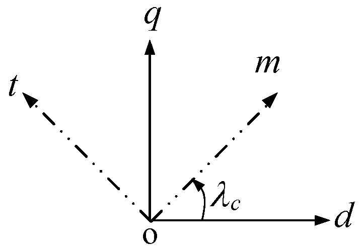
As shown in Figure 2, λ c is the angle between the mt reference frame and the rotor reference frame. Using the following transformation:
x m t = T 1 x d q ,   u m t = T 2 u d q
where T 1 = [ e j λ c 0 0 0 e j λ c 0 0 0 e j λ c ] , T 2 = [ e j λ c 0 0 e j λ c ] , the synchronous reference frame state-space model (SSSM) is obtained, that is:
x ˙ m t = A m t x m t + B m t u m t
where A m t = [ r p s ( l c s l r l c m 2 ) K j ( p p ω r + λ ˙ c ) r p s l p m l c m K r p s l c s l p m K r c s l p m l c m K r c s ( l p s l r l p m 2 ) K + j ( p c ω r λ ˙ c ) r c s l p s l c m K r r l c s l p m K r r l p s l c m K r r l p s l c s K j λ ˙ c ] , B m t = [ 1 0 0 1 0 0 ] , x m t = [ ψ p s m t ψ c s m t ψ r m t ] T , u m t = [ u p s m t u c s m t ] T , A m t = T 1 A d q T 1 1 T 1 T ˙ 1 1 , B m t = T 1 B d q T 2 1 .
The electromagnetic torque can be re-expressed as:
T e = p p l c s l p m K Im { ψ p s m t ( ψ r m t ) * } p c l p s l c m K Im { ψ c s m t ( ψ r m t ) * } + ( p p + p c ) l p m l c m K Im { ( ψ p s m t ) * ψ c s m t }
and the motion equation is same as Equation (8). Because the rotation transformation does not affect the cross-product operation of two vectors, the torque expressions before and after rotation transformation, Equations (10) and (13), are the same form. In the mt reference frame, all variables of state equations are DC values under the static state. The static working point is easily obtained.

3. Static Load Capacity of Brushless Doubly Fed Machine

Using the SSSM of the previous section, the relationships among flux, torque and speed under the static state can be easily obtained. The load capacity of BDFM is analyzed by applying these relationships.
When the mt reference frame orients on the stator flux of the CM ψ c s mt , there is:
ψ c s m t = ψ c s m + j ψ c s t = ψ c s + j 0
where ψ c s is the stator flux amplitude of the CM. To analyze the static load capacity of BDFM, let the derivatives of the states are zero in Equation (12), and the static equations of BDFM are obtained as follows:
( r p s ( l c s l r l c m 2 ) K + j ω p ) ψ p s m t r p s l p m l c m K ψ c s + r p s l c s l p m K ψ r m t + u p s m t = 0
r c s l p m l c m K ψ p s m t ( r c s ( l p s l r l p m 2 ) K j ω c ) ψ c s + r c s l p s l c m K ψ r m t + u c s m t = 0
r r l c s l p m K ψ p s m t + r r l p s l c m K ψ c s ( r r l p s l c s K + j λ ˙ c ) ψ r m t = 0
where λ ˙ c is the slip velocity of the stator flux of the CM relative to the d axis of the rotor reference frame. In practice, the CM is supplied through a converter (the stator flux amplitude of the CM will be a constant by a stator flux of the CM feedback control), and the stator of the PM is connected directly to the power grid. Therefore, the voltage amplitude and frequency of the PM are constant, and there are the following constraint conditions:
u p s 2 = u p s m 2 + u p s t 2 , ω p = p p ω r + λ ˙ c = 2 π f p
where f p and ω p are the frequency and electrical angular velocity of the PM power supply, respectively. The BDFM has the operation characteristics of the synchronous motor, when the frequency of the PM and the motor speed are constant, the slip is constant, and from Equation (13), the torque is adjusted by the angle between the stator fluxes of the CM and the PM. Even though the flux amplitudes of PM and CM can keep constant, the output torque are limited. Otherwise, with the increase of the stator current, the voltage drop in stator resistance of the PM will lead to the reduction of the PM exciting level, and the output torque is further limited. In the following discussion, the limitation of the stator voltage of the CM will not be taken into account. That is to say, for any ψ p s m t , ψ r m t and ψ c s , there is always a supply voltage of the CM u c s m t that meets Equation (16), Equation (16) need not be considered. Nevertheless, for a certain stator flux of the CM ψ c s , speed ω r , by Equations (13), (15), (17) and (18), the solutions of ψ p s m t and ψ r m t (its components of m axis and t axis are real number) are only obtained in a certain range of torque. Then we can get the upper and lower limits of BDFM’s load capacity.
For getting the solutions of the stator flux of the PM ψ p s m t and the rotor flux ψ r m t , firstly, by multiplying the conjugate of ( r r l p s l c s K j λ ˙ c ) in both sides of Equation (17), the relationship between the rotor flux, the stator fluxes of the PM and CM, and the slip velocity is given as:
ψ r m t = r r l c s l p m λ ˙ c 2 K 2 + r r 2 l p s 2 l c s 2 ( r r l p s l c s j λ ˙ c K ) ψ p s m t + r r l p s l c m λ ˙ c 2 K 2 + r r 2 l p s 2 l c s 2 ( r r l p s l c s j λ ˙ c K ) ψ c s
Substituting Equation (19) into Equation (13), to eliminate the rotor flux ψ r m t , the electromagnetic torque can be expressed as:
T e = a 1 ψ p s 2 + Re { ( a 2 + j a 3 ) ψ p s m t ψ c s } a 4 ψ c s 2
where ψ p s 2 = ψ p s m 2 + ψ p s t 2 , a 1 = p p r r l c s 2 l p m 2 λ ˙ c ( r r 2 l p s 2 l c s 2 + λ ˙ c 2 K 2 ) , a 2 = ( p p p c ) r r l p s l c s l p m l c m λ ˙ c ( r r 2 l p s 2 l c s 2 + λ ˙ c 2 K 2 ) , a 3 = ( p p + p c ) l p m l c m λ ˙ c 2 K ( r r 2 l p s 2 l c s 2 + λ ˙ c 2 K 2 ) , a 4 = p c r r l p s 2 l c m 2 λ ˙ c ( r r 2 l p s 2 l c s 2 + λ ˙ c 2 K 2 ) , a i ( i = 1 , 2 , , 4 ) are only the functions of the motor parameters and slip velocity, and they are constant under the static state.
In the electromagnetic torque expression of Equation (20), there are four terms. The first term a 1 ψ p s 2 is the asynchronous torque of the PM, and the fourth term a 4 ψ c s 2 is the asynchronous torque of the CM. The second and third terms Re { ( a 2 + j a 3 ) ψ p s m t ψ c s } are the synchronous torque. It can be seen that, for a certain slip velocity and stator flux amplitude, the two asynchronous torques are constant, and always have opposite directions. When the slip velocity λ ˙ c is relatively large (this is the majority working condition of BDFM), and the rotor impedance relatively small ( r r is relatively small), a 1 , a 2 , and a 4 will be small, and the asynchronous torque of BDFM can be neglected. Therefore, the electromagnetic torque of the BDFM is controlled by the synchronous torque, and it is only determined by the angle between the two stator fluxes.
Secondly, substituting Equation (19) into Equation (15), to eliminate the rotor flux ψ r m t , the relationship between the stator voltage of the PM and the stator fluxes is obtained as:
u p s m t = ( b 1 + j b 2 ) ψ p s m t + ( b 3 + j b 4 ) ψ c s
where b 1 = r p s λ ˙ c 2 K ( l c s l r l c m 2 ) + r p s r r 2 l p s l c s 2 ( r r 2 l p s 2 l c s 2 + λ ˙ c 2 K 2 ) , b 2 = ω p ( r r 2 l p s 2 l c s 2 + λ ˙ c 2 K 2 ) + r p s r r l c s 2 l p m 2 λ ˙ c ( r r 2 l p s 2 l c s 2 + λ ˙ c 2 K 2 ) , b 3 = r p s l p m l c m λ ˙ c 2 K ( r r 2 l p s 2 l c s 2 + λ ˙ c 2 K 2 ) , b 4 = r p s r r l p s l c s l p m l c m λ ˙ c ( r r 2 l p s 2 l c s 2 + λ ˙ c 2 K 2 ) , b i ( i = 1 , 2 , , 4 ) are only the functions of motor parameters and slip velocity.
Furthermore, substituting Equation (21) into the constraint condition Equation (18), the relationship between the stator voltage amplitude of the PM and the stator fluxes is obtained as:
u p s 2 = ( b 1 2 + b 2 2 ) ψ p s 2 + 2 Re { [ ( b 1 b 3 + b 2 b 4 ) j ( b 1 b 4 b 2 b 3 ) ] ψ p s m t } ψ c s + ( b 3 2 + b 4 2 ) ψ c s 2
Combining Equations (20) and (22) and letting T e = T l (under the static state, the electromagnetic torque T e equals the load torque T l ), the following equation is obtained:
a 1 ( k 1 2 + k 2 2 ) k 2 2 ψ p s m 2 + ( a 2 k 2 2 ψ c s 2 a 1 k 1 k 3 a 3 k 1 k 2 ψ c s ) k 2 2 ψ p s m + a 1 k 3 2 k 2 2 + a 3 k 3 ψ c s k 2 a 4 ψ c s 2 T l = 0
where k 1 = a 2 ( b 1 2 + b 2 2 ) 2 a 1 ( b 1 b 3 + b 2 b 4 ) ψ c s , k 2 = a 3 ( b 1 2 + b 2 2 ) 2 a 1 ( b 2 b 3 b 1 b 4 ) ψ c s , k 3 = ( b 1 2 + b 2 2 ) T l a 1 u p s 2 + a 4 ( b 1 2 + b 2 2 ) + a 1 ( b 3 2 + b 4 2 ) ψ c s 2 , k i ( i = 1 , 2 , 3 ) are not only the functions of the motor parameters and slip velocity, but also related to the stator flux amplitude of the CM, among them, the k 3 is also related to the voltage amplitude of the PM and load torque.
Equation (23) is complicated and difficult to obtain the analytical solutions. However, for a given u p s 2 , stator flux of the CM ψ c s , speed ω r (so the slip velocity λ ˙ c is also given) and torque T l , the numerical solution of ψ p s m can be solved. Then, substituting the solved ψ p s m into Equation (22), the ψ p s t is obtained, and substituting the solved ψ p s m and ψ p s t into Equation (19), the ψ r m t is obtained. These solutions meet the conditions of Equations (15), (17) and (18). All real number solutions constitute the possible static operation range of the BDFM (Stability is temporarily not considered). When the torque arrives at a certain value, the solved ψ p s m is not a real number, that is, the torque reaches the upper limit or lower limit of the static solution range, corresponding to the maximum or minimum torque of the BDFM. In this way, looking for the static working range of the BDFM is transformed to find the real solutions of Equation (23).

4. Losing Control Problems of Conventional Direct Torque Control (DTC) for BDFM and Its Improved Strategy

As mentioned above, the model of the BDFM is complex, and in practice its parameters are difficult to measure. DTC has less dependence on motor parameters, and specifically, it is not dependent on the rotor parameters. This is especially important for the BDFM control system design. However, compared to the induction motor, the flux and torque losing control problems of the BDFM’s conventional DTC are more evident (There may exist some time intervals, where the flux and the torque cannot be controlled simultaneously, the flux and torque ripples exceed the hysteresis ring). In Reference [26], the losing control problems of the BDFM are investigated, and flux priority and torque priority strategies are proposed. However, these strategies cannot eliminate the flux and torque ripples. In this paper, the causes of losing control problems are analyzed deeply, and an improved control strategy of DTC is proposed to solve these problems.
In the mt reference frame, the CM stator flux amplitude and the torque derivative equations about time are as follows:
d ψ c s d t = ψ c s ψ c s m t d ψ c s m t d t = 1 ψ c s Re { ( ψ c s m t ) * ψ ˙ c s m t }
d T e d t = T e ψ p s m t d ψ p s m t d t + T e ψ c s m t d ψ c s m t d t + T e ψ r m t d ψ r m t d t = p p l p m l c s K Im { ( ψ r m t ) * ψ ˙ p s m t ( ψ p s m t ) * ψ ˙ r m t } p c l p s l c m K Im { ( ψ r m t ) * ψ ˙ c s m t ( ψ c s m t ) * ψ ˙ r m t } + ( p p + p c ) l p m l c m K Im { ( ψ p s m t ) * ψ ˙ c s m t ( ψ c s m t ) * ψ ˙ p s m t }
Substituting Equation (12) into Equations (24) and (25), we have that:
d ψ c s d t = 1 ψ c s [ α 1 Re { ψ c s m t ( ψ r m t ) * } α 2 Re { ψ p s m t ( ψ c s m t ) * } + α 3 ψ c s 2 + Re { u c s m t ( ψ c s m t ) * } ]
d T e d t = α 4 T e + α 5 [ Im { u c s m t ( ψ r m t ) * } p c ω r Re { ψ c s m t ( ψ r m t ) * } ] + α 6 Im { ψ c s m t ( ψ r m t ) * } α 7 Im { ψ p s m t ( ψ r m t ) * } α 8 [ Im { u p s m t ( ψ r m t ) * } + p p ω r Re { ψ p s m t ( ψ r m t ) * } ] + α 9 [ Im { ψ p s m t ( u c s m t ) * } Im { ψ c s m t ( u p s m t ) * } + ( p p + p c ) ω r Re { ψ p s m t ( ψ c s m t ) * } ]
where α 1 = r c s l p s l c m K , α 2 = r c s l p m l c m K , α 3 = r c s ( l p m 2 l p s l r ) K , α 4 = r p s ( l c s l r l c m 2 ) + r c s ( l p s l r l p m 2 ) + r r l p s l c s K , α 5 = p c l p s l c m K , α 6 = p c r p s l c m K , α 7 = p p r c s l p m K , α 8 = p p l c s l p m K , α 9 = ( p p + p c ) l p m l c m K , α i ( i = 1 , 2 , , 9 ) are only the functions of motor parameters, and independent of motor working points. Obviously, the CM stator flux amplitude and the torque derivatives have no relationship with the selection of coordinate, thus, the derivatives of Equations (26) and (27) can be transformed into the two-phase static reference system (αβ reference frame), so we have:
d ψ c s d t = 1 ψ c s [ α 1 Re { ψ c s α β ( ψ r α β ) * } α 2 Re { ψ p s α β ( ψ c s α β ) * } + α 3 ψ c s 2 + Re { u c s α β ( ψ c s α β ) * } ]
d T e d t = α 4 T e + α 5 [ Im { u c s α β ( ψ r α β ) * } p c ω r Re { ψ c s α β ( ψ r α β ) * } ] + α 6 Im { ψ c s α β ( ψ r α β ) * } α 7 Im { ψ p s α β ( ψ r α β ) * } α 8 [ Im { u p s α β ( ψ r α β ) * } + p p ω r Re { ψ p s α β ( ψ r α β ) * } ] + α 9 [ Im { ψ p s α β ( u c s α β ) * } Im { ψ c s α β ( u p s α β ) * } + ( p p + p c ) ω r Re { ψ p s α β ( ψ c s α β ) * } ]
For the static working points (discussed in the previous section), the output torque and the motor speed are constant. Using the stator flux of the CM as the reference (the initial phase angle of the stator flux of the CM is zero), the amplitudes of all vectors, the angles among these vectors are const, and they can be expressed as:
ψ p s α β = ψ p s e j ( ω c t + δ ) ,   ψ c s α β = ψ c s e j ω c t ,   ψ r α β = ψ r e j ( ω c t + θ ) ,   u p s α β = u p s e j ( ω c t + δ + γ )
where ω c is the synchronous angular speed of the stator voltage of the CM, δ is the angle between the stator flux of the PM and stator flux of the CM, θ is the angle between the stator flux of the CM and rotor flux, and γ is the angle between the stator voltage and stator flux of the PM. The stator of the CM is supplied through a converter, and the converter output voltage vectors are as follows:
u c s α β = 2 3 V b u s e j ( π / 3 ( n 1 ) )
where V b u s is the DC bus voltage, and n = 1 , 2 , , 6 correspond to the six fundamental nonzero voltage vectors (three-phase two level converter, six fundamental voltage vectors and two zero voltage vectors). Substituting Equations (30) and (31) into Equations (28) and (29), we obtain the stator flux amplitude of the CM and torque derivative equations around the static working points are as follows:
d ψ c s d t = 2 3 V b u s cos ( ω c t π / 3 ( n 1 ) ) + A
d T e d t = 2 3 α 5 V b u s ψ r sin ( π / 3 ( n 1 ) ω c t θ ) + 2 3 α 9 V b u s ψ p s sin ( ω c t + δ π / 3 ( n 1 ) ) + B
where:
A = α 1 ψ r cos θ α 2 ψ p s cos δ + α 3 ψ c s
B = α 4 T e + α 9 ψ p s ψ c s [ ( p p ω r + p c ω r ) cos δ + ω p sin ( δ + γ ) ] α 5 p c ω r ψ c s ψ r cos θ α 6 ψ c s ψ r sin θ + α 8 ψ p s ψ r [ ω p sin ( θ δ γ ) p p ω r cos ( θ δ ) ] + α 7 ψ p s ψ r sin ( θ δ )
are constant (but change with working points), and they are the derivative values of the stator flux amplitude of the CM and torque when the converter output voltage is the two zero voltage vectors, respectively.
As mentioned above, if the asynchronous torque is neglected, we have:
d ψ c s d t = 2 3 V b u s cos ( ω c t π / 3 ( n 1 ) ) + A
d T e d t = 2 3 α 9 V b u s ψ p s sin ( ω c t + δ π / 3 ( n 1 ) ) + B
where:
A = α 2 ψ p s cos δ + α 3 ψ c s
B = α 4 T e + α 9 ψ p s ψ c s [ ( p p ω r + p c ω r ) cos δ + ω p sin ( δ + γ ) ]
For a large power motor, the stator resistance of the CM is small. Because α 1 , α 2 and α 3 are proportional to the stator resistance of the CM and the stator flux amplitude will decrease when the converter output voltage is zero, A is always small and negative. The stator flux amplitude of the CM and the torque derivatives are sinusoidal with the synchronous angle ω c t , and when the converter output voltage u c s α β is different fundamental voltage vectors ( n = 1 , 2 , , 6 ), the electric angles of these derivative curves are 60 ° apart in turn. For a given voltage vector u c s α β , the angle between the stator flux amplitude of the CM derivative curves and the torque derivative curves changes with the variation of the working points.
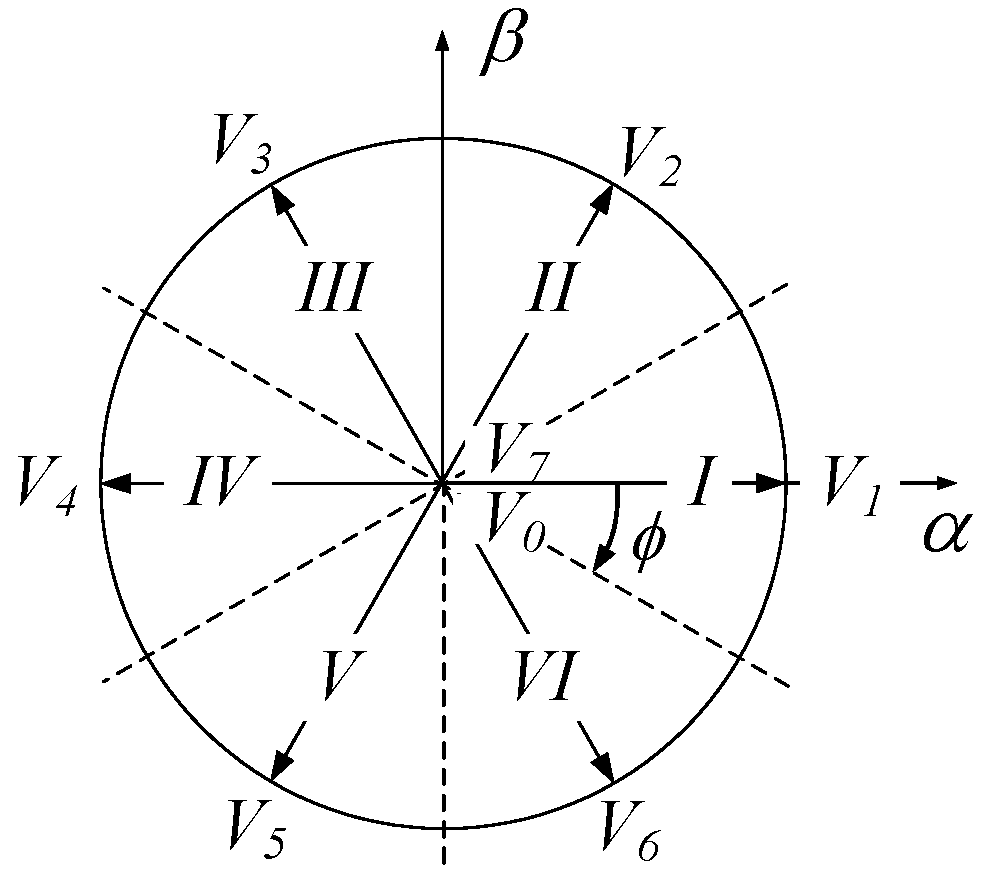
For conventional DTC, there are the six nonzero voltage vectors, V1V6. As shown in Figure 3, the two-phase static reference frame is divided into six sectors (sector IVI), each sector occupies 60 ° , and the angle ϕ between the boundary of sector I and the α axis is 30 ° .
In the follow discussion, a rated power 3.7 kW BDFM is used as an example, the parameters of which are shown in the Appendix A, and the supply voltage and frequency of the PM are 220 V/50 Hz. Using the Equations (32) and (33), the stator flux amplitude of the CM and the torque derivative curves are shown in Figure 4a,b.Where the stator flux of the CM is 1.2 Wb, the motor speed is 62.8 rad/s (subsynchronous), and the output torques are 30 Nm (motoring mode) and –30 Nm (generating mode). It is clear that the flux derivative curves of the two nonzero voltage vectors with 180 ° phase difference are symmetrical about the line of d ψ c s / d t = A . In each sector, there must be two flux derivative curves, their signs will be changed, and the two corresponding voltage vectors cannot be selected, because they cannot provide a fixed response direction of flux. Similarly, the torque derivative curves of the two fundamental nonzero voltage vectors with 180 ° phase difference are symmetrical about the line of d T e / d t = B , there must be two torque derivative curves in each sector, their signs will be changed, and the two corresponding voltage vectors cannot be selected. In each sector, if the above four voltage vectors are not the same, as shown in Figure 4a,b, there will be four voltage vectors, they cannot be selected. Obviously, the rest of two voltage vectors cannot satisfy the four kinds of control requirements: decreasing in flux and torque, decreasing in flux and increasing in torque, increasing in flux and decreasing in torque, and increasing in flux and torque. The selection of the voltage vector can only make the losing control time as short as possible. In Figure 4c,d, the flux derivative curves of sector I are enlarged to show the regions of the flux losing control more clearly.
Thus, the voltage vector switch tables can be obtained under the motoring mode and generating mode, as shown in Table 1 and Table 2, called the conventional DTC. From the sector I to the sector VI, the electric angles of voltage vectors selected for the same control requirements are 60 ° apart in turn. The control system is shown in Figure 5. Under the motoring mode, the flux will lose control when an increase in flux and a decrease in torque, or an increase in flux and an increase in torque are desired, corresponding to the third and fourth rows in Table 1 (that is the circular region in Figure 4c). Under the generating mode, the flux will lose control when an increase in flux and a decrease in torque, or an increase in flux and an increase in torque are desired, corresponding to the third and fourth rows in Table 2 (that is the circular region in Figure 4d).
From Figure 4a,b, it can be also seen that if the angle φ is increased, the flux losing control can be eliminated under the action of the voltage vector V6, but the flux losing control will be serious under the action of the voltage vector V2. On the contrary, if the angle φ is decreased, the flux losing control can be eliminated under the action of the voltage vector V2, but the flux losing control will be serious under the action of the voltage vector V6. Therefore, it is useless to solve the flux losing control by changing the angle φ. Because the DC component A of the flux amplitude derivative is relatively small in general situations, the time interval of the flux losing control is short, and the range of the flux fluctuation is small. When the load is light, the torque will not lose control.
With the increase in torque, the DC components A and B are increase, the phase angles of the flux derivative curves remain unchanged, and the torque derivative curves move right or left (motoring or generating modes) relative to the flux derivative curves. In Figure 6a,b,the stator flux of the CM and the torque derivative curves are shown, where the stator flux of the CM is 1.2 Wb, the motor speed is 62.8 rad/s (subsynchronous), and the output torques are 55 Nm (motoring mode) and −99 Nm (generating mode). The voltage vector switch tables can be obtained, which are same as the Table 1 and Table 2. When the load is heavy, the flux and the torque will all lose control. Under the motoring mode, the torque will lose control when a decrease in flux and an increase in torque, or an increase in flux and a decrease in torque are desired, corresponding to the second and third rows in Table 1 (that is the losing control regions I and II in Figure 6a). Under the generating mode, the torque will lose control when a decrease in flux and a decrease in torque, or an increase in flux and an increase in torque are desired, corresponding to the first and fourth rows in Table 2 (that is the losing control regions II and I in Figure 6b).
Similarly, from Figure 6a,b, it can be also seen that if the angle φ is increased, the flux losing control can be eliminated under the action of the voltage vector V6, but the flux losing control will be serious under the action of the voltage vector V2, and the torque losing control will also be serious under the action of the voltage vectors V3 and V6. On the contrary, if the angle φ is decreased, the flux losing control can be eliminated under the action of the voltage vector V2, and the torque losing control also can be eliminated under the action of the voltage vector V3 and V6, but the flux losing control will be more serious under the action of the voltage vector V6. Therefore, the losing control problems of the conventional DTC cannot be solved by changing the angle φ.
From the analysis above, it can be seen that the BDFM’s conventional DTC easily loses control, because the selected voltage vector are fewer and the sector is relatively wide. The losing control problems cannot be improved by increasing the switch sectors, or by changing the angle φ between the boundary of sector I and the α axis. And increasing the DC bus voltage, the time of losing control will decrease, but the losing control phenomena would not disappear. Therefore, for the BDFM’s DTC control system, the flux and torque losing control phenomenon always exist and are inevitable.
Without changing the converter topology, the new voltage vectors are synthesized by the six fundamental voltage vectors. As shown in Figure 7, the V12 is synthesized by the V1 and V2, the V23 is synthesized by the V2 and V3, the V34 is synthesized by the V3 and V4, the V45 is synthesized by the V4 and V5, the V56 is synthesized by the V5 and V6, and the V61 is synthesized by the V6 and V1. The duty ratio of two fundamental voltage vectors related to every synthesized voltage vector are 50 % . The six fundamental voltage vectors and the six synthesized voltage vectors, there are twelve voltage vectors. At the same time, the switch sectors also increase to twelve, each sector occupies 30 ° , and the angle φ is 15 ° . The following will point out that the losing control problems can be solved by increasing the number of voltage vectors and the switch sectors simultaneously, and combined with the appropriate choice of angle φ.
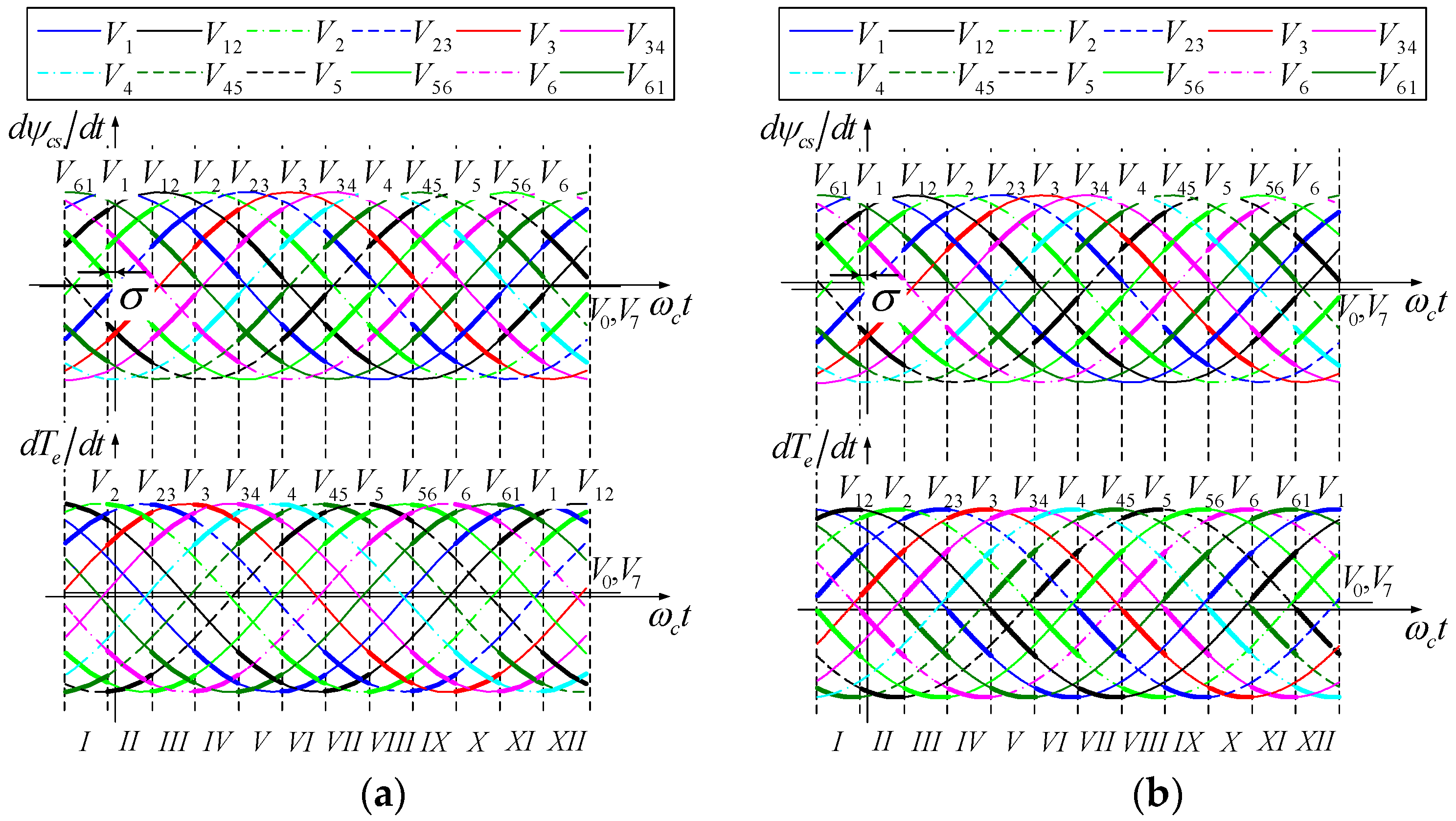
After adding synthesized voltage vectors, the stator flux amplitude of the CM and the torque derivative curves are shown in Figure 8a,b, where the stator flux of the CM is 1.2 Wb, the motor speed is 62.8 rad/s (subsynchronous), the output torques are 30 Nm and 59 Nm (light load and heavy load under the motoring mode), and the angle φ = −15°–σ = −21 has been chosen properly.
Similarly, in each sector, there are also two flux amplitude and two toque derivative curves, their signs change inevitably, the corresponding four voltage vectors cannot be selected. Among the rest of eight voltage vectors, the vectors, they can satisfy the control requirements of flux and torque and their derivative curves are farther from the horizontal axis, will be selected. In this way, the selection of voltage vector makes that the control effect is more obvious (good effectiveness and quick adjustment), and the effectiveness can be maintained (strong robustness) when the operating conditions (load torque, speed, etc.) change. Then twelve sectors voltage vector switch tables can be obtained, as shown in Table 3 and Table 4, and called SVDTC control strategy. From the sector I to the sector XII, the electric angles of selected voltage vectors for the same control requirements are 30 ° apart in turn. If the angle φ is still 15 ° , the sector I as an example, the selected voltage vectors can satisfy the control requirements of torque, but the flux will lose control under the action of the voltage vector V56. Because the DC component A of the flux derivative is relatively small in general situations, only a small adjustment of φ is needed in the basis of 15 ° . The analysis of the generating mode is similar to the motoring mode, the figures of its derivative curves are omitted here. The control system of SVDTC is shown in Figure 9.
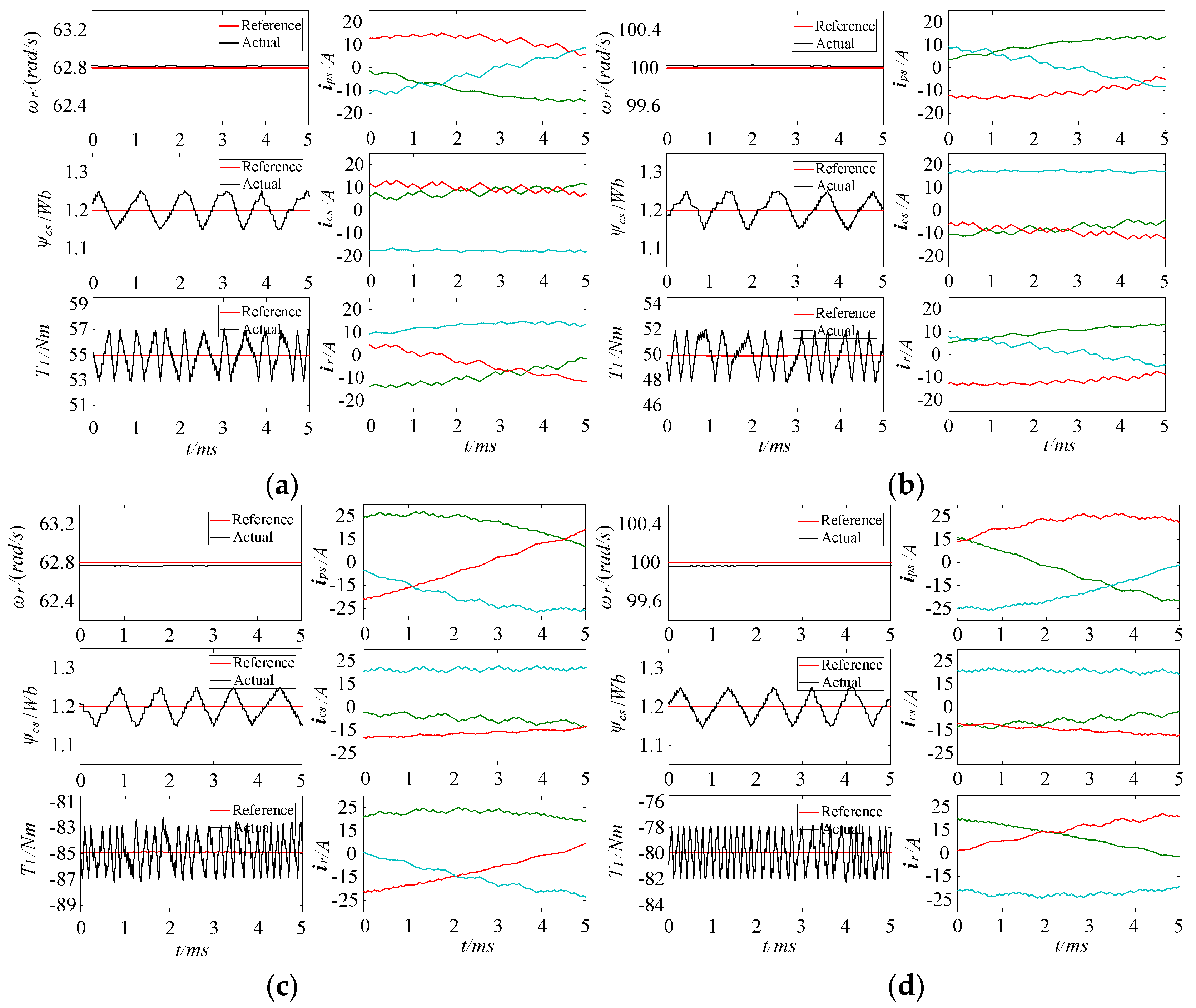
The following simulation will illustrate that the SVDTC not only can solve the flux and torque losing control problems of the conventional DTC, but also can make the BDFM output torque reach the theoretical output capacity limits.

5. Simulation Experiments

5.1. Numerical Calculation of Static Operation Ranges

The BDFM of the Appendix A is still used as an example, the supply voltage and frequency of the PM are 220 V/50 Hz, a specific calculation result is shown in Figure 10. It can be seen that the range of possible maximum output torque decreases gradually with the increase in motor speed when the stator flux amplitude of the CM is constant. The range of possible maximum output torque first increases and then decreases gradually with the increase in the stator flux amplitude of the CM when the motor speed is constant. When the stator flux amplitude of the CM increases to 1.8 Wb, the maximum output torque of the BDFM reaches the peak value of 72 Nm. Compared with the maximum torque, the range of possible minimum output torque increases gradually with the increase in the stator flux amplitude of the CM, and decreases gradually with the increase in speed.
For large power motor, the situation of above is somewhat different. In this case, the stator and rotor resistances are very small, the ranges of possible maximum and minimum output torque will tend to be equal, independent of the motor speed, and increase with the increase in the stator flux amplitude of the CM.
Obviously, the stable working points of BDFM must locate in the interior of the maximum and minimum torque curves, and the percentage of the stable operation range is related to the control method. When the stator flux amplitude of the CM is 1.2 Wb, the maximum and minimum torque curves, the stability operation ranges of the BDFM under constant V/f open loop control and under conventional DTC are shown in Figure 11. As we seen that, using the constant V/f open loop control, the stability operation rangeis near the synchronous speed, and occupies a small part of the entire static solution range, using conventional DTC, the torque will lose control before it reaches the limits of the static solution region.

5.2. Simulation Test of Synthetic Vector Direct Torque Control (SVDTC)

To display the performance of the proposed new control strategy SVDTC, simulation tests have been carried out. The control performances of the conventional DTC and SVDTC are compared under various kinds of operating conditions. The power motor is connected to a 220 V/50 Hz power supply, and the control motor is supplied through a bridge converter, and the DC voltage of the converter is 500 V. The stator flux observers of the PM and CM use voltage current models, ψ p s α β = ( u p s α β r p s i p s α β ) d t and ψ c s α β = ( u c s α β r c s i c s α β ) d t . In order to overcome the problem of dc drifts of a pure integral, the stator fluxes are estimated by a adaptive compensation integrator, where the cutoff angular velocity of low-pass filter ω C F is 1 rad/s, and the PI parameters of regulator are k p = 0.01 , k I = 1 [29]. The torque is calculated by the cross product of fluxes and currents, T e = p p Im { ( ψ p s α β ) * i p s α β } + p c Im { ( ψ c s α β ) * i c s α β } . The speed outer loop is adopted, the PI parameters of speed loop are k p = 2 , k I = 20 . The upper and lower limits of flux and torque hysteresis comparators are 0.05 and −0.05, 2 and −2. The parameters of BDFM are shown in the Appendix A.

5.2.1. Simulation Waveforms of DTC and SVDTC

Figure 12 and Figure 13 display the simulation results of conventional DTC and SVDTC, respectively. In this simulation, the reference value of ψ c s is 1.2 Wb, the reference value of ω r is 62.8 rad/s or 100 rad/s (subsynchronous or supersynchronous) under different load torque.
Under the four conditions of different torques and different speeds, the partial enlarged simulation waveforms of the conventional DTC are illustrated in Figure 12a–d. It can be seen that, the deviations of torque will exceed the upper and lower limits of hysteresis comparator, the speed fluctuation appears when the torque loses control. And the torque losing control has two forms, from little to big, and from big to little, which is associated with the different change trends of torque derivative curves in the losing control region, as shown in Figure 12a,b. Figure 12e–h show the torque waveforms in a 360 ° of electric angles under the four work conditions, there are six torque ripples in each of them. With the increase in the torque, the torque losing control becomes serious and continues for a longer time, the maximum torque ripple reaches 9 Nm, and the maximum proportion of losing control time is over 70%.
The partial enlarged simulation waveforms of the SVDTC are illustrated in Figure 13a–d. It can be seen that the SVDTC can effectively solve the losing control problems, whether the motor operates in motoring or generating modes, and it makes the deviations of the stator flux of the CM and torque are restricted in the hysteresis ring width simultaneously. The motor speed and stator flux amplitude of the CM properly follow the reference value. When a fundamental voltage vector is selected, until the deviations of the flux or torque reach the limits of hysteresis comparators, the voltage vector will switch once. In this case, the switching frequency is related to the hysteresis ring width. When a synthesized voltage vector is selected, two related fundamental voltage vectors are modulated, the duty ratio of the two fundamental voltage vectors are 50 % , and the modulation frequency is 20 KHz. In this case, the switching frequency is fixed, until the hysteresis comparator state changes and other voltage vector is selected. Figure 13e–h also show the torque waveforms of several periods under the four conditions. This demonstrates that the effectiveness can be maintained in a wide range by the SVDTC control strategy when the operating conditions (load torque, speed) change. The proposed SVDTC is effective in coping with losing control problems. The stability and robustness of the control system are improved.

5.2.2. Speed Command and Load Torque Disturbance Responses of SVDTC

Figure 14 shows the dynamic response of the BDFM to a step speed command. In this simulation, the reference value of ψ c s is 1.2 Wb, the reference value of ω r changes from 62.8 rad/s to 100 rad/s at 0.21 s, and the load torque is 5 Nm, the PI regulator output limiting values are ±53 (the maximum torque is 54 Nm at 100 rad/s when the flux is 1.2 Wb). It can be seen that, when the speed command changes from subsynchronous to supersynchronous, the actual speed rapidly follows the reference value without overshoots, and the current phase sequence of the CM changes. The motor accelerates at 53 Nm, and then the torque returns back 5 Nm after approximately 0.06 s.
Figure 15 shows the regulating performance of the BDFM to a step change in load torque. In this simulation, the reference value of ψ c s is 1.2 Wb, the reference value of ω r is 62.8 rad/s, and the load torque changes from 5 Nm to 30 Nm at 0.1 s. The system stability is validated under a step load torque disturbance. The speed returns to the reference speed after several dynamic fluctuations, and the speed regulator is able to compensate for the load torque disturbance in a time period of approximately 0.3 s.
Figure 14 and Figure 15 also show the stator currents of the PM and CM, and the rotor current. Figure 14 and Figure 15 demonstrate that the system of SVDTC has a good response characteristics for step speed command, and a good regulating performance under step load torque disturbance. The stator flux amplitude of the CM follows the reference value well, and it is almost unaffected by the variations of speed and torque.

5.2.3. Output Capacity of the SVDTC of BDFM System

In addition to the losing control problem, the systems of conventional DTC and CM constant V/f open loop control will lose stability when the load torque increases to a certain value. For example, under the conventional DTC, when the flux ψ c s is 1.2 Wb, the speed ω r is 62.8 rad/s, if the load torque exceeds 55 Nm, the torque will diverge.
The SVDTC not only can solve the flux and torque losing control problems of the conventional DTC, but also can make the output torque of the BDFM reach the theoretical output capacity limits. In order to validate this conclusion, simulation tests have been carried out.
In this simulation, the reference value of ψ c s is 1.2 Wb, the reference value of ω r is 62.8 rad/s, and the load torque is changed gradually. According to Figure 11, the maximum output torque of BDFM is 59 Nm under the above working conditions. Figure 16 shows that the actual output torque is always able to follow reference torque when the load torque changes from 30 Nm to 50 Nm at 0.2 s, and then changes from 50 Nm to 58 Nm at 1 s. In the interior of the maximum and minimum output torque curves of Figure 11, setting some test points on the boundaries, we find that the results are same, and the waveforms are omitted here. The SVDTC can make the output torque of the BDFM reach the theoretical output capacity limits, but conventional DTC cannot.

6. Conclusions

For different rotor structures BDFM, the method of taking conjugation transformation of the complex variables of CM or PM has universality. Using this method, the synchronous reference frame state-space model, called SSSM, is obtained in this paper. By the description of the SSSM, the analysis method of the output capacity limits of BDFM is given and used to test the performance of the control strategy. The improved DTC strategy, called SVDTC, can solve the losing problems of the flux and torque, and keep the advantage of conventional DTC, such as simple structure, less dependence on motor parameters, and strong robustness. The dynamic performance of SVDTC is tested over a wide range of speeds from subsynchronous to supersynchronous, and also under conditions of sudden load change. The theoretical output capacity limits can be reached by the SVDTC control strategy. These results have significant meaning for the BDFM’s design and development and also for the control strategy study.

Author Contributions

The conjugation transformation and the synchronous reference frame state-space model, the analysis method of output capacity limits and the SVDTC of BDFM belong to Chaoying Xia. The derivation of output capacity related results of BDFM and all the simulations are completed by Xiaoxin Hou. Both of the authors wrote and revised the manuscript.

Conflicts of Interest

The authors declare no conflict of interest.

Appendix A

BDFM parameters:
pp = 1, pc = 3, rps = 1.77 Ω, rcs = 1.64 Ω, lps = 0.461 H, lcs = 0.136 H, lpm = 0.4575 H, lcm = 0.115 H, rr = 6.0028 Ω, ll = 0.597 H, J = 0.05 kg·m2.

References

  1. Zhang, A.L.; Wang, X.; Jia, W.X.; Ma, Y. Indirect stator-quantities control for the brushless doubly fed induction machine. IEEE Trans. Power Electron. 2014, 3, 1392–1401. [Google Scholar] [CrossRef]
  2. Abdi, S.; Abdi, E.; Oraee, A.; McMahon, R. Equivalent circuit parameters for large brushless doubly fed machines (bdfms). IEEE Trans. Energy Convers. 2014, 3, 706–715. [Google Scholar] [CrossRef]
  3. Hashemnia, M.N.; Tahami, F.; Oyarbide, E. Investigation of core loss effect on steady-state characteristics of inverter fed brushless doubly fed machines. IEEE Trans. Energy Convers. 2014, 1, 57–64. [Google Scholar] [CrossRef]
  4. Zhao, R.L.; Zhang, A.L.; Ma, Y.; Wang, X.; Yan, J.; Ma, Z.Z. The dynamic control of reactive power for the brushless doubly fed induction machine with indirect stator-quantities control scheme. IEEE Trans. Power Electron. 2015, 9, 5046–5057. [Google Scholar] [CrossRef]
  5. Xiong, F.; Wang, X.F. Design of a low-harmonic-content wound rotor for the brushless doubly fed generator. IEEE Trans. Energy Convers. 2014, 1, 158–168. [Google Scholar] [CrossRef]
  6. McMahon, R.; Tavner, P.; Abdi, E.; Malliband, P.; Barker, D. Characterising brushless doubly fed machine rotors. IET Electr. Power Appl. 2013, 7, 535–543. [Google Scholar] [CrossRef]
  7. Shao, S.Y.; Abdi, E.; Barati, F.; McMahon, R. Stator-flux-oriented vector control for brushless doubly fed induction generator. IEEE Trans. Ind. Electron. 2009, 10, 4220–4228. [Google Scholar] [CrossRef]
  8. Shao, S.Y.; Abdi, E.; McMahon, R. Operation of brushless doubly-fed machine for drive applications. In Proceedings of the Fourth IET Conference on Power Electronics, Machines and Drives, York, UK, 2–4 April 2008; pp. 340–344.
  9. Jallali, F.; Bouchhima, A.; Masmoudi, A. Steady-state operation of the brushless cascaded doubly fed machine: A survey. COMPEL Int. J. Comput. Math. Electr. Electron. Eng. 2011, 1, 222–245. [Google Scholar] [CrossRef]
  10. Roberts, P.C.; McMahon, R.A.; Tavner, P.J.; Maciejowski, J.M.; Flack, T.J. Equivalent circuit for the brushless doubly fed machine (BDFM) including parameter estimation and experimental verification. IEE Proc. Electr. Power Appl. 2005, 4, 933–942. [Google Scholar] [CrossRef]
  11. Li, R.; Wallace, A.; Spee, R.; Wang, Y. Two-axis model development of cage-rotor brushless doubly-fed machines. IEEE Trans. Energy Convers. 1991, 3, 453–460. [Google Scholar] [CrossRef]
  12. Zhou, D.S.; Spee, R. Synchronous frame model and decoupled control development for doubly-fed machines. In Proceedings of the 25th Annual IEEE Power Electronics Specialists Conference, Taipei, China, 20–25 June 1994.
  13. Zhou, D.; Spee, R.; Alexander, G.C.; Wallace, A.K. A simplified method for dynamic control of brushless double-fed machines. In Proceedings of the 1996 IEEE IECON 22nd International Conference on Industrial Electronics, Control, and Instrumentation, Taipei, China, 5–10 August 1996; pp. 946–951.
  14. Poza, J.; Oyarbide, E.; Roye, D. New vector control algorithm for brushless doubly-fed machines. In Proceedings of the 2002 28th Annual Conference of the IEEE Industrial Electronics Society, Seville, Spain, 5–8 November 2002; pp. 1138–1143.
  15. Poza, J.; Oyarbide, E.; Roye, D.; Rodriguez, M. Unified reference frame dq model of the brushless doubly fed machine. IEE Proc. Electr. Power Appl. 2006, 153, 726–734. [Google Scholar] [CrossRef]
  16. Li, R.; Wallace, A.; Spee, R. Determination of converter control algorithms for brushless doubly-fed induction motor drives using Floquet and Lyapunov techniques. IEEE Trans. Power Electron. 1995, 1, 78–85. [Google Scholar]
  17. Sarasola, I.; Poza, J.; Oyarbide, E.; Rodriguez, M.A. Stability analysis of a brushless doubly-fed machine under closed loop scalar current control. In Proceedings of the 32nd Annual Conference on IEEE Industrial Electronics, Paris, France, 6–10 October 2006.
  18. Poza, J.; Oarbide, E.; Roye, D.; Sarasola, I. Stability analysis of a BDFM under open-loop voltage control. In Proceedings of the 2005 European Conference on Power Electronics and Applications, Dresden, Germany, 11–14 September 2005.
  19. Williamson, S.; Ferreira, A. Generalised theory of the brushless doubly-fed machine. Part 2: Model verification and performance. IEE Proc. Electr. Power Appl. 1997, 2, 123–129. [Google Scholar] [CrossRef]
  20. McMahon, R.A.; Roberts, P.C.; Wang, X.; Tavner, P.J. Performance of BDFM as generator and motor. IEE Proc. Electr. Power Appl. 2006, 2, 289–299. [Google Scholar] [CrossRef]
  21. Roberts, P.C.; Flack, T.J.; Maciejowski, J.M.; McMahon, R.A. Two stabilising control strategies for the brushless doubly-fed machine (BDFM). In Proceedings of the 2002 International Conference on Power Electronics, Machines and Drives, Bath, Britain, 16–18 April 2006; pp. 341–346.
  22. Xia, C.Y.; Guo, H.Y. Feedback linearization control approach for brushless double-fed machine. Int. J. Precis. Eng. Manuf. 2015, 8, 1699–1709. [Google Scholar] [CrossRef]
  23. Takahashi, I.; Noguchi, T. A new quick-response and high-efficiency control strategy of an induction motor. IEEE Trans. Ind. Appl. 1986, 5, 820–827. [Google Scholar] [CrossRef]
  24. Brassfield, W.R.; Spee, R.; Habetler, T.G. Direct torque control for brushless doubly-fed machines. IEEE Trans. Ind. Appl. 1996, 5, 1098–1104. [Google Scholar] [CrossRef]
  25. Abad, G.; Rodríguez, M.Á.; Poza, J. Two-level VSC based predictive direct torque control of the doubly fed induction machine with reduced torque and flux ripples at low constant switching frequency. IEEE Trans. Power Electron. 2008, 3, 1050–1061. [Google Scholar] [CrossRef]
  26. Sarasola, I.; Poza, J.; Rodríguez, M.Á.; Abad, G. Direct torque control design and experimental evaluation for the brushless doubly fed machine. Energy Convers. Manag. 2011, 2, 1226–1234. [Google Scholar] [CrossRef]
  27. Fattahi, S.J.; Khayyat, A.A. Direct torque control of brushless doubly-fed induction machines using fuzzy logic. In Proceedings of the 2011 IEEE Ninth International Conference on Power Electronics and Drive Systems (PEDS), Singapore, 5–8 December 2011.
  28. Sarasola, I.; Poza, J.; Rodríguez, M.Á. Predictive direct torque control for brushless doubly fed machine with reduced torque ripple at constant switching frequency. In Proceedings of the 2007 IEEE International Symposium on Industrial Electronics, Vigo, Spain, 4–7 June 2007.
  29. Hu, J.; Wu, B. New integration algorithms for estimating motor flux over a wide speed range. IEEE Trans. Power Electron. 1998, 5, 969–977. [Google Scholar]
Figure 1. Variables of stator and rotor windings, stator ABC reference frame, static αβ reference frame, rotor abc reference frame and rotor dq reference frame.
Energies 09 00966 g001
Figure 2. Relationships between the CM synchronous reference frame and the rotor reference frame.
Energies 09 00966 g002
Figure 3. Six sectors in the two-phase static reference frame.
Energies 09 00966 g003
Figure 4. Stator flux of the CM and torque derivative curves (light load). (a) Motoring mode (Te = 30 Nm); (b) Generating mode (Te = −30 Nm); (c) Partial enlarged (Te = 30 Nm); (d) Partial enlarged (Te = −30 Nm).
Energies 09 00966 g004
Figure 5. Control system of conventional DTC.
Energies 09 00966 g005
Figure 6. Stator flux of the CM and torque derivative curves (heavy load). (a) Motoring mode (Te = 59 Nm); (b) Generating mode (Te = −99 Nm).
Energies 09 00966 g006
Figure 7. Twelve sectors in the two-phase static reference frame.
Energies 09 00966 g007
Figure 8. Stator flux of the CM and torque derivative curves. (a) Motoring mode (Te = 30 Nm); (b) Motoring mode (Te = 59 Nm).
Energies 09 00966 g008
Figure 9. Control system of SVDTC.
Energies 09 00966 g009
Figure 10. Maximum and minimum torque curve surfaces of a BDFM.
Energies 09 00966 g010
Figure 11. Stability operation ranges under constant V/f control and under conventional DTC.
Energies 09 00966 g011
Figure 12. Simulation waveforms of conventional DTC. (a) 55 Nm, 62.8 rad/s (motoring mode); (b) 50 Nm, 100 rad/s (motoring mode); (c) −85 Nm, 62.8 rad/s (generating mode); (d) −80 Nm, 100 rad/s (generating mode); (e) 55 Nm, 62.8 rad/s; (f) 50 Nm, 100 rad/s; (g) −85 Nm, 62.8 rad/s; (h) −80 Nm, 100 rad/s.
Energies 09 00966 g012aEnergies 09 00966 g012b
Figure 13. Simulation waveforms of SVDTC. (a) 55 Nm, 62.8 rad/s (motoring mode); (b) 50 Nm, 100 rad/s (motoring mode); (c) −85 Nm, 62.8 rad/s (generating mode); (d) −80 Nm, 100 rad/s (generating mode); (e) 55 Nm, 62.8 rad/s; (f) 50 Nm, 100 rad/s; (g) −85 Nm, 62.8 rad/s; (h) −80 Nm, 100 rad/s.
Energies 09 00966 g013aEnergies 09 00966 g013b
Figure 14. Speed changes from 62.8 rad/s to 100 rad/s at 5 Nm load.
Energies 09 00966 g014
Figure 15. Load torque changes from 5 Nm to 30 Nm at 62.8 rad/s.
Energies 09 00966 g015
Figure 16. Simulation waveforms of SVDTC at limit torque.
Energies 09 00966 g016
Table 1. Voltage vector switch table (motoring mode).
Output of Hysteresis ComparatorSix Sectors
FluxTorqueIIIIIIIVVVI
–1−1V5V6V1V2V3V4
1V3V4V5V6V1V2
1−1V6V1V2V3V4V5
1V2V3V4V5V6V1
Note: “1” and “−1” indicate the increased and decreased flux or torque, respectively.
Table 2. Voltage vector switch table (generating mode).
Output of Hysteresis ComparatorSix Sectors
FluxTorqueIIIIIIIVVVI
–1–1V3V4V5V6V1V2
1V5V6V1V2V3V4
1–1V2V3V4V5V6V1
1V6V1V2V3V4V5
Note: “1” and “−1” indicate the increased and decreased flux or torque, respectively.
Table 3. Twelve sectors voltage vector switch table (motoring mode).
Output of Hysteresis ComparatorTwelve Sectors
FluxTorqueIIIIIIIVVVIVIIVIIIIXXXIXII
−1–1V45V5V56V6V61V1V12V2V23V3V34V4
1V23V3V34V4V45V5V56V6V61V1V12V2
1–1V56V6V61V1V12V2V23V3V34V4V45V5
1V12V2V23V3V34V4V45V5V56V6V61V1
Table 4. Twelve sectors voltage vector switch table (generating mode).
Output of Hysteresis ComparatorTwelve Sectors
FluxTorqueIIIIIIIVVVIVIIVIIIIXXXIXII
–1–1V23V3V34V4V45V5V56V6V61V1V12V2
1V45V5V56V6V61V1V12V2V23V3V34V4
1–1V12V2V23V3V34V4V45V5V56V6V61V1
1V56V6V61V1V12V2V23V3V34V4V45V5

