
Implementing a Novel Hybrid Maximum Power Point Tracking Technique in DSP via Simulink/MATLAB under Partially Shaded Conditions

 , ,
, ,
Abstract
:
1. Introduction
2. PV System


| Parameters | Values |
|---|---|
| Power at maximum point, MPP | 43 W |
| Voltage at maximum point, VMPP | 17.4 V |
| Current at maximum point, IMPP | 2.48 A |
| Open circuit voltage, VOC | 21.7 V |
| Short circuit current, ISC | 2.65 A |
| Temperature coefficient of VOC | −0.0821 V/°C |
| Temperature coefficient of ISC | 0.00106 A/°C |
| Number of cells per module | 36 |
3. System Configuration
3.1. DC-DC Boost Converter
3.2. Load Value in a Standalone System


4. Proposed Hybrid MPPT Method


5. Implementing DSP via Simulink/MATLAB

5.1. Analog-to-Digital Converter (ADC)
5.2. ePWM Block
5.2.1. Module
5.2.2. Timer Period
5.2.3. Counting Mode


6. Simulation Results


7. Experimental Results


| Items | Scenario (Figure) | SOP | TGMPP (s) | Pave_PSC (W) | Pripp_PSC (W) | Irradiation (W/m2) | |
|---|---|---|---|---|---|---|---|
| System | |||||||
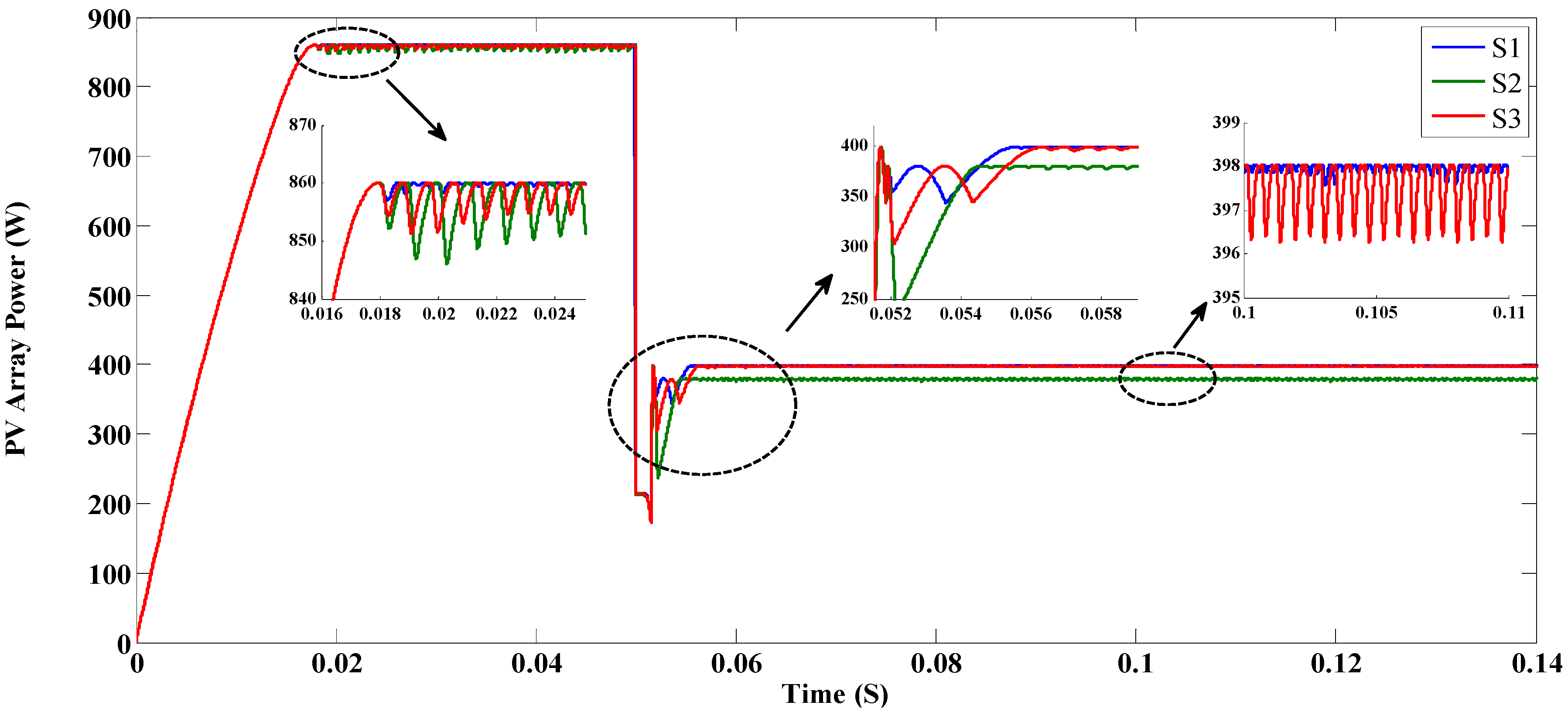
| S1 | 18 | Successful | 8.18 | 554.2 | 4.6 | 1000 | |
| S2 | 18 | Successful | 11.56 | 554.2 | 10.4 | 1000 | |
| S3 | 18 | Successful | 17.62 | 554.2 | 8.6 | 1000 | |
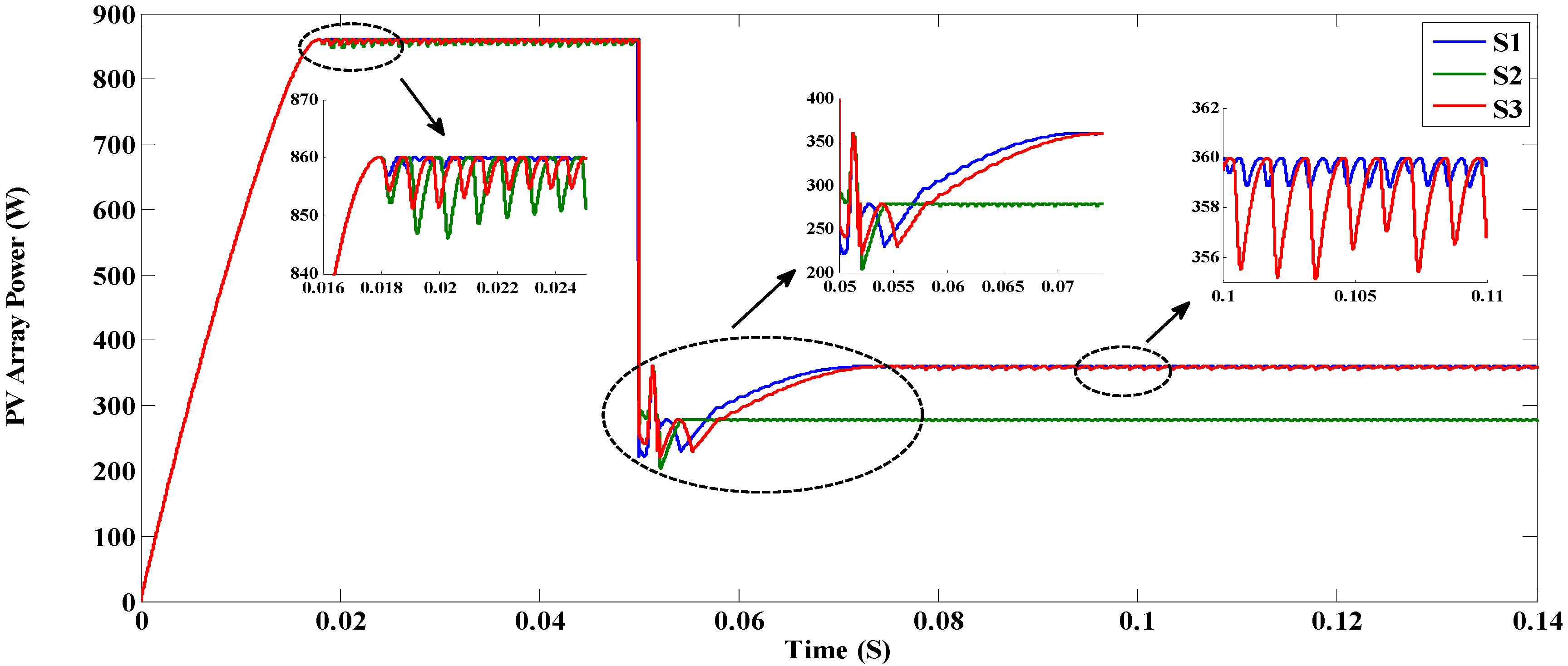
| S1 | 20 | Successful | 22.64 | 360 | 4.5 | 1000 | |
| S2 | 20 | Failed | - | 278.8 | - | 1000 | |
| S3 | 20 | Successful | 24.68 | 360 | 11.6 | 1000 | |
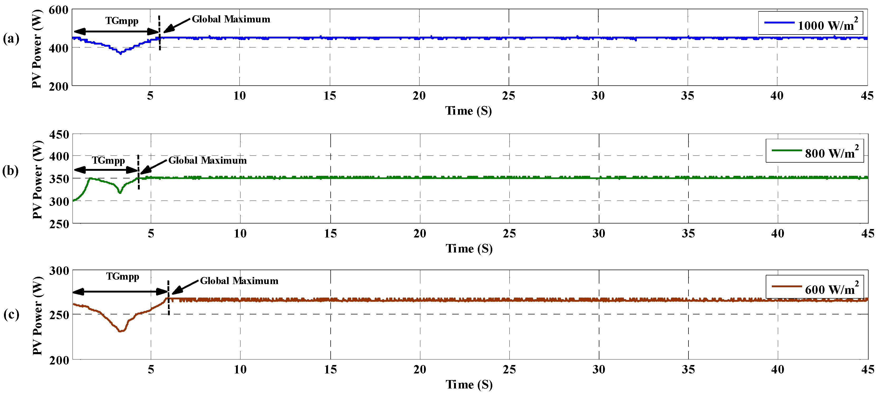
| S1 | 22.a | Successful | 5.46 | 429.96 | 2.8 | 1000 | |
| S1 | 22.b | Successful | 4.34 | 349.16 | 3.2 | 800 | |
| S1 | 22.c | Successful | 6 | 265.82 | 4.2 | 600 | |
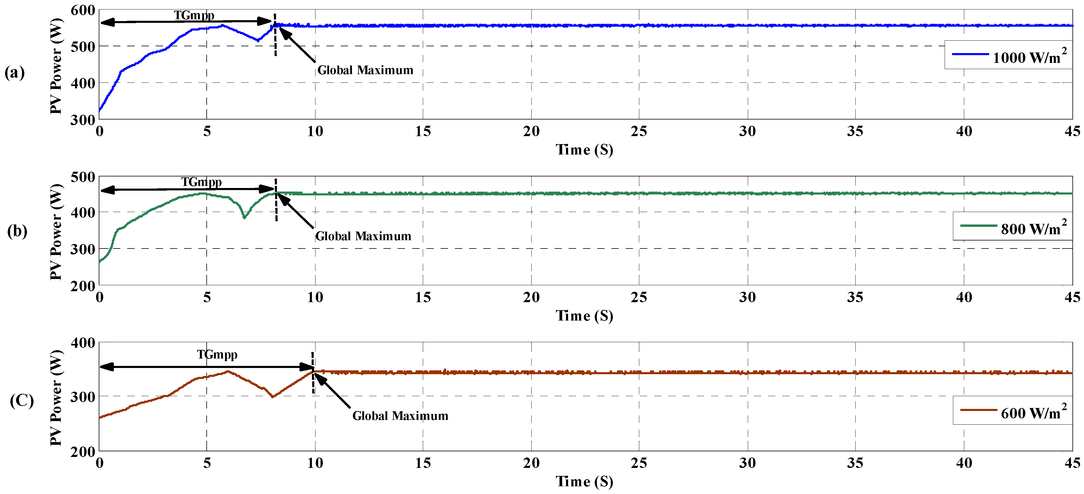
| S1 | 24.a | Successful | 8.14 | 554.2 | 2.6 | 1000 | |
| S1 | 24.b | Successful | 8.18 | 449.7 | 2.8 | 800 | |
| S1 | 24.c | Successful | 9.88 | 340.9 | 3.2 | 600 | |
| S1 | 26.a | Successful | 15.68 | 417.2 | 2.8 | 1000 | |
| S1 | 26.b | Successful | 16.68 | 338 | 3.6 | 800 | |
8. Conclusions
Acknowledgments
Author Contributions
Conflicts of Interest
References
- Banos, R.; Manzano-Agugliaro, F.; Montoya, F.; Gil, C.; Alcayde, A.; Gómez, J. Optimization methods applied to renewable and sustainable energy: A review. Renew. Sustain. Energy Rev. 2011, 15, 1753–1766. [Google Scholar] [CrossRef]
- Tomabechi, K. Energy resources in the future. Energies 2010, 3, 686–695. [Google Scholar] [CrossRef]
- Liu, G.; Nguang, S.K.; Partridge, A. A general modeling method for I–V characteristics of geometrically and electrically configured photovoltaic arrays. Energy Convers. Manag. 2011, 52, 3439–3445. [Google Scholar] [CrossRef]
- Sullivan, C.R.; Awerbuch, J.J.; Latham, A.M. Decrease in photovoltaic power output from ripple: Simple general calculation and the effect of partial shading. IEEE Transactions on Power Electronics 2013, 28, 740–747. [Google Scholar] [CrossRef]
- Karatepe, E.; Hiyama, T.; Boztepe, M.; Çolak, M. Voltage based power compensation system for photovoltaic generation system under partially shaded insolation conditions. Energy Convers. Manag. 2008, 49, 2307–2316. [Google Scholar] [CrossRef]
- Martínez-Moreno, F.; Muñoz, J.; Lorenzo, E. Experimental model to estimate shading losses on PV arrays. Sol. Energy Mater. Sol. Cells 2010, 94, 2298–2303. [Google Scholar] [CrossRef] [Green Version]
- Piegari, L.; Rizzo, R.; Spina, I.; Tricoli, P. Optimized adaptive perturb and observe maximum power point tracking control for photovoltaic generation. Energies 2015, 8, 3418–3436. [Google Scholar] [CrossRef]
- Lee, J.-S.; Lee, K.B. Variable DC-link voltage algorithm with a wide range of maximum power point tracking for a two-string pv system. Energies 2013, 6, 58–78. [Google Scholar] [CrossRef]
- Yau, H.-T.; Wu, C.-H. Comparison of extremum-seeking control techniques for maximum power point tracking in photovoltaic systems. Energies 2011, 4, 2180–2195. [Google Scholar] [CrossRef]
- Esram, T.; Chapman, P.L. Comparison of photovoltaic array maximum power point tracking techniques. IEEE Trans. Energy Convers. 2007, 22, 439–449. [Google Scholar] [CrossRef]
- Rezk, H.; Eltamaly, A.M. A comprehensive comparison of different MPPT techniques for photovoltaic systems. Solar Energy 2015, 112, 1–11. [Google Scholar] [CrossRef]
- Ahmed, J.; Salam, Z. A critical evaluation on maximum power point tracking methods for partial shading in PV systems. Renew. Sustain. Energy Rev. 2015, 47, 933–953. [Google Scholar] [CrossRef]
- Ishaque, K.; Salam, Z. A review of maximum power point tracking techniques of PV system for uniform insolation and partial shading condition. Renew. Sustain. Energy Rev. 2013, 19, 475–488. [Google Scholar] [CrossRef]
- Liu, Y.-H.; Chen, J.-H.; Huang, J.-W. A review of maximum power point tracking techniques for use in partially shaded conditions. Renew. Sustain. Energy Rev. 2015, 41, 436–453. [Google Scholar] [CrossRef]
- Hohm, D.; Ropp, M. Comparative study of maximum power point tracking algorithms using an experimental, programmable, maximum power point tracking test bed. In Proceedings of the 2000 IEEE Twenty-Eighth Photovoltaic Specialists Conference, Anchorage, AK, USA, 15–22 September 2000; pp. 1699–1702.
- Houssamo, I.; Locment, F.; Sechilariu, M. Maximum power tracking for photovoltaic power system: Development and experimental comparison of two algorithms. Renew. Energy 2010, 35, 2381–2387. [Google Scholar] [CrossRef]
- Jiang, J.; Huang, T.; Hsiao, Y.; Chen, C. Maximum power tracking for photovoltaic power systems. Tamkang J. Sci. Eng. 2005, 8, 147–153. [Google Scholar]
- Aganah, K.; Leedy, A.W. A constant voltage maximum power point tracking method for solar powered systems. In Proceedings of the 2011 IEEE 43rd Southeastern Symposium on System Theory (SSST 2011), Auburn, AL, USA, 14–16 March 2011; pp. 125–130.
- Masoum, M.A.; Dehbonei, H.; Fuchs, E.F. Theoretical and experimental analyses of photovoltaic systems with voltageand current-based maximum power-point tracking. IEEE Trans. Energy Convers. 2002, 17, 514–522. [Google Scholar] [CrossRef]
- Orozco, M.A.; Vázquez, J.; Salmerón, P. MPP tracker of a PV system using sliding mode control with minimum transient response. Int. Rev. Model. Simul. 2010, 3, 1468–1475. [Google Scholar]
- Bianconi, E.; Calvente, J.; Giral, R.; Mamarelis, E.; Petrone, G.; Ramos-Paja, C.A.; Spagnuolo, G.; Vitelli, M. Perturb and observe MPPT algorithm with a current controller based on the sliding mode. Int. J. Electr. Power Energy Syst. 2013, 44, 346–356. [Google Scholar] [CrossRef]
- Bose, B.K.; Szczesny, P.M.; Steigerwald, R.L. Microcomputer control of a residential photovoltaic power conditioning system. IEEE Trans. Ind. Appl. 1985, IA-21, 1182–1191. [Google Scholar] [CrossRef]
- Guenounou, O.; Dahhou, B.; Chabour, F. Adaptive fuzzy controller based MPPT for photovoltaic systems. Energy Convers. Manag. 2014, 78, 843–850. [Google Scholar] [CrossRef]
- Liu, C.-L.; Chen, J.-H.; Liu, Y.-H.; Yang, Z.-Z. An asymmetrical fuzzy-logic-control-based mppt algorithm for photovoltaic systems. Energies 2014, 7, 2177–2193. [Google Scholar] [CrossRef]
- Hiyama, T.; Kitabayashi, K. Neural network based estimation of maximum power generation from PV module using environmental information. IEEE Trans. Energy Convers. 1997, 12, 241–247. [Google Scholar] [CrossRef]
- Jiang, L.L.; Maskell, D.L.; Patra, J.C. A novel ant colony optimization-based maximum power point tracking for photovoltaic systems under partially shaded conditions. Energy and Buildings 2013, 58, 227–236. [Google Scholar] [CrossRef]
- Miyatake, M.; Veerachary, M.; Toriumi, F.; Fujii, N.; Ko, H. Maximum power point tracking of multiple photovoltaic arrays: A PSO approach. IEEE Trans. Aerosp. Electron. Syst. 2011, 47, 367–380. [Google Scholar] [CrossRef]
- Muthuramalingam, M.; Manoharan, P. Comparative analysis of distributed MPPT controllers for partially shaded stand alone photovoltaic systems. Energy Convers. Manag. 2014, 86, 286–299. [Google Scholar] [CrossRef]
- Tsang, K.; Chan, W. Model based rapid maximum power point tracking for photovoltaic systems. Energy Convers. Manag. 2013, 70, 83–89. [Google Scholar] [CrossRef]
- Kobayashi, K.; Takano, I.; Sawada, Y. A study of a two stage maximum power point tracking control of a photovoltaic system under partially shaded insolation conditions. Sol. Energy Mater. Sol. Cells 2006, 90, 2975–2988. [Google Scholar] [CrossRef]
- Miyatake, M.; Inada, T.; Hiratsuka, I.; Zhao, H.; Otsuka, H.; Nakano, M. Control characteristics of a fibonacci-search-based maximum power point tracker when a photovoltaic array is partially shaded. In Proceedings of the 2004 IEEE 4th International Power Electronics and Motion Control Conference (IPEMC 2004), Xi’an, China, 14–16 August 2004; pp. 816–821.
- Nguyen, T.L.; Low, K.-S. A global maximum power point tracking scheme employing direct search algorithm for photovoltaic systems. IEEE Trans. Ind. Electron. 2010, 57, 3456–3467. [Google Scholar] [CrossRef]
- Lin, C.-H.; Huang, C.-H.; Du, Y.-C.; Chen, J.-L. Maximum photovoltaic power tracking for the PV array using the fractional-order incremental conductance method. Appl. Energy 2011, 88, 4840–4847. [Google Scholar] [CrossRef]
- Ji, Y.-H.; Jung, D.-Y.; Kim, J.-G.; Kim, J.-H.; Lee, T.-W.; Won, C.-Y. A real maximum power point tracking method for mismatching compensation in PV array under partially shaded conditions. IEEE Trans. Power Electron. 2011, 26, 1001–1009. [Google Scholar] [CrossRef]
- Patel, H.; Agarwal, V. Maximum power point tracking scheme for PV systems operating under partially shaded conditions. IEEE Trans. Ind. Electron. 2008, 55, 1689–1698. [Google Scholar] [CrossRef]
- Sarvi, M.; Ahmadi, S.; Abdi, S. A PSO-based maximum power point tracking for photovoltaic systems under environmental and partially shaded conditions. Prog. Photovoltaics 2015, 23, 201–214. [Google Scholar] [CrossRef]
- Hajighorbani, S.; Radzi, M.A.M.; Kadir, M.Z.A.A.; Shafie, S. Dual search maximum power point (dsmpp) algorithm based on mathematical analysis under shaded conditions. Energies 2015, 8, 12116–12146. [Google Scholar] [CrossRef]
- Castaner, L.; Silvestre, S. Front Matter; Wiley Online Library: Hoboken, NJ, USA, 2002. [Google Scholar]
- Chowdhury, S.; Chowdhury, S.; Taylor, G.; Song, Y. Mathematical modelling and performance evaluation of a stand-alone polycrystalline PV plant with MPPT facility. In Proceedings of the 2008 IEEE Power and Energy Society General Meeting-Conversion and Delivery of Electrical Energy in the 21st Century, Pittsburgh, PA, USA, 20–24 July 2008; pp. 1–7.
- Jung, J.-H.; Ahmed, S. Model construction of single crystalline photovoltaic panels for real-time simulation. In Proceedings of the 2010 IEEE Energy Conversion Congress and Exposition (ECCE 2010), Delft, The Netherlands, 25–27 August 2010; pp. 342–349.
- González-Longatt, F.M. Model of photovoltaic module in matlab. II CIBELEC 2005, 2005, 1–5. [Google Scholar]
- Skoplaki, E.; Palyvos, J. On the temperature dependence of photovoltaic module electrical performance: A review of efficiency/power correlations. Solar Energy 2009, 83, 614–624. [Google Scholar] [CrossRef]
- Kroposki, B.; Myers, D.; Emery, K.; Mrig, L.; Whitaker, C.; Newmiller, J. Photovoltaic module energy rating methodology development. In Proceedings of the 1996 IEEE Twenty Fifth Photovoltaic Specialists Conference, Washington, DC, USA, 13–17 May 1996; pp. 1311–1314.
- Barbieri, F.; Chandrasena, R.P.; Shahnia, F.; Rajakaruna, S.; Ghosh, A. Application notes and recommendations on using TMS320f28335 digital signal processor to control voltage source converters. In Proceedings of the 2014 Australasian Universities Power Engineering Conference (AUPEC 2014), Perth, Australia, 28 September–1 October 2014; pp. 1–7.
- Instruments, T. Ti-TMS320f28335 Data Sheet; Texas Instruments, Inc.: Dallas, TX, USA, 2007. [Google Scholar]
© 2016 by the authors; licensee MDPI, Basel, Switzerland. This article is an open access article distributed under the terms and conditions of the Creative Commons by Attribution (CC-BY) license (http://creativecommons.org/licenses/by/4.0/).
Share and Cite
Hajighorbani, S.; Mohd Radzi, M.A.; Ab Kadir, M.Z.A.; Shafie, S.; Mohd Zainuri, M.A.A. Implementing a Novel Hybrid Maximum Power Point Tracking Technique in DSP via Simulink/MATLAB under Partially Shaded Conditions. Energies 2016, 9, 85. https://doi.org/10.3390/en9020085
Hajighorbani S, Mohd Radzi MA, Ab Kadir MZA, Shafie S, Mohd Zainuri MAA. Implementing a Novel Hybrid Maximum Power Point Tracking Technique in DSP via Simulink/MATLAB under Partially Shaded Conditions. Energies. 2016; 9(2):85. https://doi.org/10.3390/en9020085
Chicago/Turabian StyleHajighorbani, Shahrooz, Mohd Amran Mohd Radzi, Mohd Zainal Abidin Ab Kadir, Suhaidi Shafie, and Muhammad Ammirrul Atiqi Mohd Zainuri. 2016. "Implementing a Novel Hybrid Maximum Power Point Tracking Technique in DSP via Simulink/MATLAB under Partially Shaded Conditions" Energies 9, no. 2: 85. https://doi.org/10.3390/en9020085