The Driving Forces of Changes in CO₂ Emissions in China: A Structural Decomposition Analysis

Abstract

Understanding the drivers of changes in CO₂ emissions is vital for a range of stakeholders. Hence, this paper explores the main drivers of CO₂ emissions in China using structural decomposition analysis based on constant price and non-comparative input-output tables. The driving forces at both nationwide and industrial levels are divided into nine effects. To investigate the effects from an energy perspective, all nine effects are further decomposed into three kinds of fossil fuels. Our empirical results show that the energy intensity effect can significantly stimulate emission reduction. Though the energy structure effect is weak, the trend of which over time shows that the energy structure is shifting to low carbon. Additionally, among final demand effect, the urban consumption, investment, and export expansion effects predominantly overwhelm other effects and contribute significantly to CO₂ emissions. Although the short term Leontief effects fluctuate greatly, the total Leontief effect in 1997–2010 reveals that it can significantly contribute to CO₂ emissions. Finally, detailed and concrete policy implications for CO₂ emission reduction are provided.

1. Introduction

Anthropogenic climate change, including global warming, acid deposition and ozone depletion is one of the major challenges the planet faces [1,2]. Essentially speaking, global warming, as the most urgent problem for human beings, is because of a large amount of Greenhouse Gases (GHGs) caused by burning fossil fuels and human activities [3]. International Energy Agency (IEA) estimates that China’s CO₂ emissions will reach 11.4 billion tons in 2030 without any emission reduction constraints [4]. Against this backdrop, it seems more critical to analyze influencing factors of CO₂ emission changes from multiple points of view and different level.

With the introduction of an extended input–output framework, research on energy consumption and CO₂ emissions using input–output method is feasible [5,6]. A first group of studies, called static input–output analysis, which, based on the hypothesis of structural stability, analyzed the impact of changes in the flow variables on the final demand [7,8]. Moreover, the second method mainly analyzed the variation of energy consumption and CO₂ emissions from a perspective of production structural change [9]. Structural decomposition analysis, which contains index decomposition analysis (IDA) and structural decomposition analysis (SDA), is the main method in the second category [10,11,12].

The earliest index decomposition analysis can be traced back to the weight index proposed by Laspeyres in 1871 [13]. The main methods of index decomposition analysis can be divided into Laspeyres, Divisia, Paasche, Fisher, and Marshall–Edgeworth [14]. Of these approaches, Logarithmic Mean Divisia Index (LMDI) has increasingly become the preferred approach due to the perfect decomposition, consistency in aggregation, path independency and ability to handle the “0” values problem [15,16]. Ang [17] summarized and compared eight LMDI decomposition models. According to [18], the SDA methods are summarized as Ad hoc, D&L, LMDI, MRCI and others. Although the Ad hoc methods are standard methods in the early stage, the residual term embedded in these methods resulted in an imperfect decomposition [19]. Dietzenbacher and Los in [20] solved the problem of residual term in SDA. They proposed using all n! equivalent exact decomposition forms to achieve ideal decomposition. However, it is unwieldy when the number of influencing factors is large [21]. To solve this problem, polar decomposition and “mirror image” decomposition methods were proposed. Moreover, Su and Ang [18] provided the guidance for selecting SDA methods, and they believed that D&L model is applicable when there are more than five factors.

Structural decomposition approach can study the technical effect and the end demand effect. In particular, it also can measure the influence of indirect resource requirements caused by the end demand spillover between industries [22]. Hence, it has been widely used in the problem of energy consumption and CO₂ emissions. For instance, the related foreign studies on carbon emissions include that Cellura et al. [23] investigated air emission changes related to Italian households consumption; Cansino et al. [24] analyzed CO₂ emission in Spain; and Kopidou et al. [25] applied a decomposition analysis in the industrial sector of selected European Union countries. Moreover, related foreign studies on energy consumption mainly include Ref. [26] and Ref. [27]. Although decomposition analysis started fairly late in China, there are also many studies related to CO₂ emissions and energy consumption. Lin and Xie [28] analyzed CO₂ emissions of China’s food industry; Yuan and Zhao [29] investigated CO₂ emissions from China’s energy-intensive industries; Zhang [30] examined China’s energy consumption change from 1987 to 2007; Li et al. [31] measured China’s energy consumption under the global economic crisis; and Xie [32] detailed the driving forces of China’s energy use from 1992 to 2010. Essentially speaking, the changes experienced by the emissions and energy consumption between two periods are explained by the changes in final demand and structural coefficients [33]. In addition, SDA can also be applied to structural change [34], productivity growth [35], consumption of other sources [36], energy intensity [37,38], etc.

In view of the growing requirements of energy and environment protection in China, this paper hereby employs structural decomposition analysis to comprehensively explore CO₂ emissions growth based on constant price and non-comparative input-output tables, and investigates the intrinsic reasons for the findings from nine aspects. Meanwhile, to dig out underlying causes, the decomposition effects are further subdivided into sectors and different energy sources. In brief, all the results and analyses in this paper have reference meaning for the Chinese government depicting a blueprint for cutting the CO₂ emissions. The rest of this paper is arranged as follows: Section 2 introduces the data processing and SDA approach. Section 3 is the results. In Section 4, we provide the discussion of each effect, while in Section 5 we present conclusions and policy implications.

2. Methodology and Data

2.1. Data Processing

(1)

Step 1: Establishment of comparable price input–output table

This paper mainly used two kinds of raw data: the input–output table and energy consumption data. China’s National Bureau of Statistics has issued 1997 (17, 40, and 142 sectors), 2002 (42 and 122 sectors), and 2007 (42 sectors) input–output tables as well as 2000 (17 and 40 sectors), 2005 (42 sectors), and 2010 (42 and 65 sectors) input–output extended tables. Obviously, due to the different statistical caliber, the sector classifications in different input–output tables are different. After obtaining the necessary input–output tables, unifying the sector classifications is another important step. Considering the “Classification and Code Standard of National Economy Industry” (GB/T4754-2011) and the current sector classifications in 6 input–output tables, we disaggregate and combine the whole economy into 24 sectors. The classifications of sectors and their corresponding codes are demonstrated in

Table 1. The classifications of sectors and codes.

Classification			Sectors	Code
Primary			Agriculture, Forestry, Animal Husbandry, Fishery and Water	SEC 01
Secondary	Heavy Industry	Extractive Industry	Mining and Washing of Coal	SEC 02
			Extraction of Petroleum and Natural Gas	SEC 03
			Mining and Processing of Metal Ores	SEC 04
			Mining and Processing of Nonmetal and Other Ores	SEC 05
		Manufacturing Industry (Heavy)	Processing of Petroleum, Coking, Processing of Nuclear Fuel	SEC 06
			Manufacture of Non-metallic Mineral Products	SEC 07
			Smelting and Pressing of Metals	SEC 08
			Manufacture of Metal Products	SEC 09
			Manufacture of Special and General Purpose Machinery	SEC 10
			Manufacture of Transport Equipment	SEC 11
			Manufacture of Electrical Machinery and Equipment	SEC 12
			Chemical Industry	SEC 13
		Electricity, Heat, Water	Production and Distribution of Electric Power and Heat Power	SEC 14
	Light Industry	Manufacturing Industry (Light)	Manufacture of Foods and Tobacco	SEC 15
			Manufacture of Textile	SEC 16
			Manufacture of Leather, Fur, Feather and Related Products	SEC 17
			Manufacture of Timber and Furniture	SEC 18
			Manufacture of Paper and Educational and Sports Goods	SEC 19
			Manufacture of Communication Equipment, Computers and Other Electronic Equipment	SEC 20
			Manufacture of Measuring Instruments and Machinery for Cultural Activity and Office Work	SEC 21
			Manufacture of Artwork and Other Manufacturing	SEC 22
	Construction		Construction	SEC 23
Tertiary			Service	SEC 24

. For convenience and to conform to the expressive habits of most readers, we provide a brief classification of 24 sectors. What is noteworthy is that the final decomposition at sectoral level focuses on all the 24 sectors rather than these 7 categories.

Furthermore, the input–output table of value-type is calculated at current prices, to discount price factors and measure the change of input and output, the input–output table must be converted to comparable price input–output table. The price index for each unit is impossible when establishing the comparable price input–output table. Hence, referring to the method in Ref. [39], we presumed that the output value in a certain sector has same price index, and adjusted the sector value by rows using the same price index. By single deflation method, all 6 input–output tables have been deflated to constant 1997 prices. All price indexes are calculated by the authors according to data in “China Statistical Yearbook” [40]. The results of price indexes are shown in Appendix A.

(2)

Step 2: Collection of primary energy and carbon emission data

The energy data mainly come from “China Energy Statistical Yearbook” [41]. In order to unify the quantity of the different energy consumption, we convert all type of primary energy (coal, gasoline, kerosene, diesel, fuel oil and natural gas) into standard coal equivalent. It should be noted that only the primary energy is taken into consideration and special handling is provided for electricity data. In other words, energy usage does not include the electricity use. This was done to avoid double-counting towards the CO₂ emissions. As the most widely used secondary energy sources, over 75% of electricity in China comes from burning coal. The CO₂ embodied in electricity has been contained in coal consumption. Undoubtedly, there will be double-counting if we calculate the emission of electricity. When treating the energy intensity, we also exclude the electricity consumption and only calculate the primary energy consumption. In brief, the energy consumption in this paper only considers the primary energy that directly causes carbon emissions. The conversion factors are shown in

Table 2. The conversion factors and emission coefficients of fossil fuels.

Primary Energy Resource	Loss Coefficient	Conversion Factor	Emissions Coefficient
Coal	3.2%	0.7143 tce/t	2.7716 tCO2/tce
Gasoline	3.1%	1.4714 tce/t	2.0306 tCO2/tce
Kerosene	3.7%	1.4714 tce/t	2.1058 tCO2/tce
Diesel	3.6%	1.4571 tce/t	2.1699 tCO2/tce
Fuel Oil	3.6%	1.4286 tce/t	2.2667 tCO2/tce
Natural gas	2.0%	1.33 kgce/m3	1.6438 tCO2/tce

. According to the default value of the carbon content in “2006 IPCC Guidelines for National Greenhouse Gas Inventories”, the CO₂ emission coefficients of fossil fuels are supposed to be constant and calculated, respectively. The emissions coefficients are shown in Table 2. Furthermore, to get more precise calculation results, we introduce loss coefficients of burning fossil fuels, which are collected from State Environmental Protection Administration and National Information Center [42].

(3)

Step 3: Establishment of non-competitive Input–output Table

Input–output analysis, based on the input–output table, was put forward by Leontief in the 1930s. It set up linear relationship between all parts of the economic system and provides an effective method for analyzing the interdependent input output relationships with various branches in economic system. A simplified competitive I-O table is shown in

Table 3. A simplified competitive Input–Output Table.

I-O Table	Intermediate Use	End Use (Y)					Import	Total Output
		Consumption			Capital Formation	Export
		Rural	Urban	Government
Intermediate input	AX	RC	UC	GC	INV	EX	IM	X
Value added	V	–	–	–	–	–	–	–
Total input	XT	–	–	–	–	–	–	–

.

The product of A and X is intermediate use and inputs. V is value added vector, X is column vector of total output, and the vector of end use Y can be separated into consumption, capital formation and export. Furthermore, consumption can be divided into rural, urban and government consumption. The IM refers to the import. What is noteworthy is that the balance error in input–output table is neglected. However, according to Su and Ang [43], the implications of the competitive and non-competitive tables are not the same, and the competitive table can overestimate the carbon emission. Hence, we considered replacing competitive I-O table for non-competitive I-O table. The non-competitive I-O table is shown in

Table 4. A simplified non-competitive Input–output Table.

I-O Table	Intermediate USE	End use (Y)					Import	Total Output
		Consumption			Capital Formation	Export
		Rural	Urban	Government
Domestic Intermediate input	AdX	RCd	UCd	GCd	INVd	EX	–	X
Import Intermediate input	AmX	RCm	UCm	GCm	INVm	–	IM	–
Value added	V	–	–	–	–	–	–	–
Total input	XT	–	–	–	–	–	–	–
Energy consumption	ET	–	–	–	–	–	–	–
Energy structure	P	–	–	–	–	–	–	–
Carbon emission	CT	–	–	–	–	–	–	–

.

Different from competitive I-O table, the domestic intermediate input and import intermediate input are separated. Where, the superscript d denotes the domestic products, such as A^dX, RC^d, UC^d, GC^d, and INV^d, and the superscript m denotes the import products, such as A^mX, RC^m, UC^m, GC^m, and INV^m. Additionally, P is energy structure, which represents the proportion of fossil fuels. E is vector of primary energy consumption in all sectors and C is vector of carbon emissions in all sectors.

According to Weber et al. [44] and Lin and Sun [45], the method to separate the domestic and import intermediate is as follows:

$$M_{ij}=\{\begin{array}{c}=\frac{X_i-E{X}_i}{X_i-E{X}_i+I{M}_i}i=j\hfill \\ =0i\ne j\hfill \end{array}(i,j=1,2,\mathrm{3...},n)$$

(1)

$$A^{d}X=M\cdot AX$$

(2)

$$A^{m}X=AX-A^{d}X$$

(3)

where i represents the sectors in I-O table, A^mX denotes imports for intermediate input, and A^dX denotes domestic products for intermediate input. The derivation of end use is similar. Therefore, the product balance equation can be written as:

$$X=A^{d}X+R{C}^d+U{C}^d+G{C}^d+IN{V}^d+EX=M\cdot (AX+RC+UC+GC+INV)+EX$$

(4)

The carbon dioxide emissions are written as C, which can be formulated as:

$$C=e{m}^T{(1-A)}^{-1}Y=\mathsf{\alpha }P{e}^{T}LY=\mathsf{\alpha }P{e}^{T}X$$

(5)

where $e{m}^T$ represents the emission intensities of economic sectors. $\mathsf{\alpha }$ denotes emission coefficient of different kinds of energies. $e^T$ is energy intensity vector.

2.2. Structural Decomposition Analysis

Based on input–output theory, a static analysis method SDA was gradually developed. The SDA model, which can decompose the change of a dependent variable into the sum of various independent variables, is often used in the study of structural change. Besides, SDA approach is also used for the decomposition of employment, value-added, energy consumption, CO₂ emission, etc. Generally, the form of structural decomposition was not unique, including polar decomposition method, weighted average method, and midpoint weighting method. The polar decomposition method, put forward by Dietzenbacher and Los [20], could be used to replace the complex decomposition method. The specification of D & L method is shown in Equations (6)–(9), the derivation of SDA in this paper is shown in Appendix B.

$$y={\displaystyle \prod _{i=1}^n{x}_i}$$

(6)

$$\Delta y=y^t-y^0={\displaystyle \prod _{i=1}^n{x}_i^t-}{\displaystyle \prod _{j=1}^n{x}_j^0}$$

(7)

$$E_i=\frac{1}{2}{\displaystyle \prod _{j=1}^{i-1}{x}_j^0\cdot \Delta x_i\cdot {\displaystyle \prod _{k=i+1}^n{x}_k^t}+}\frac{1}{2}{\displaystyle \prod _{l=1}^{i-1}{x}_l^t\cdot \Delta x_i\cdot {\displaystyle \prod _{m=i+1}^n{x}_m^0}}$$

(8)

$$\Delta y={\displaystyle \sum _{i=1}^n{E}_i={\displaystyle \sum _{i=1}^n(\frac{1}{2}{\displaystyle \prod _{j=1}^{i-1}{x}_j^0\cdot \Delta x_i\cdot {\displaystyle \prod _{k=i+1}^n{x}_k^t}+}\frac{1}{2}{\displaystyle \prod _{l=1}^{i-1}{x}_l^t\cdot \Delta x_i\cdot {\displaystyle \prod _{m=i+1}^n{x}_m^0}})}}$$

(9)

where, $x_i(i=1,2\cdots n)$ are independent variables. $\Delta y$ is variation on the dependent variable, superscript 0 and t indicate the base period and calculated period. $E_i$ denotes the impact of the fluctuation of $x_i$ on $\Delta y$. Finally, the total effect $\Delta y$ can be represented as the sum of $E_i$.

3. Decomposition Results

This part shows the calculation results of the driving forces of carbon emission, including the overall decomposition results and decomposition factors in all sub-industries.

Table 5. Decomposition factors of changes in CO₂ emissions in China (10⁹ ton CO₂).

Period	EI	ES	RC	UC	GC	INV	EX	IM	Leo	TE
1997–2000	−9.629	1.521	0.673	2.126	0.77	1.754	2.448	−0.54	2.542	1.665
2000–2002	−1.857	0.839	−0.813	2.405	1.428	3.545	1.829	−0.991	−3.396	2.989
2002–2005	−8.794	0.638	0.54	2.799	1.168	7.368	9.731	−1.672	7.758	19.537
2005–2007	−16.66	−0.32	0.76	3.183	1.196	8.781	7.548	4.293	1.633	10.414
2007–2010	−17.52	−0.323	1.047	5.406	1.849	15.408	2.799	1.825	−0.757	9.734
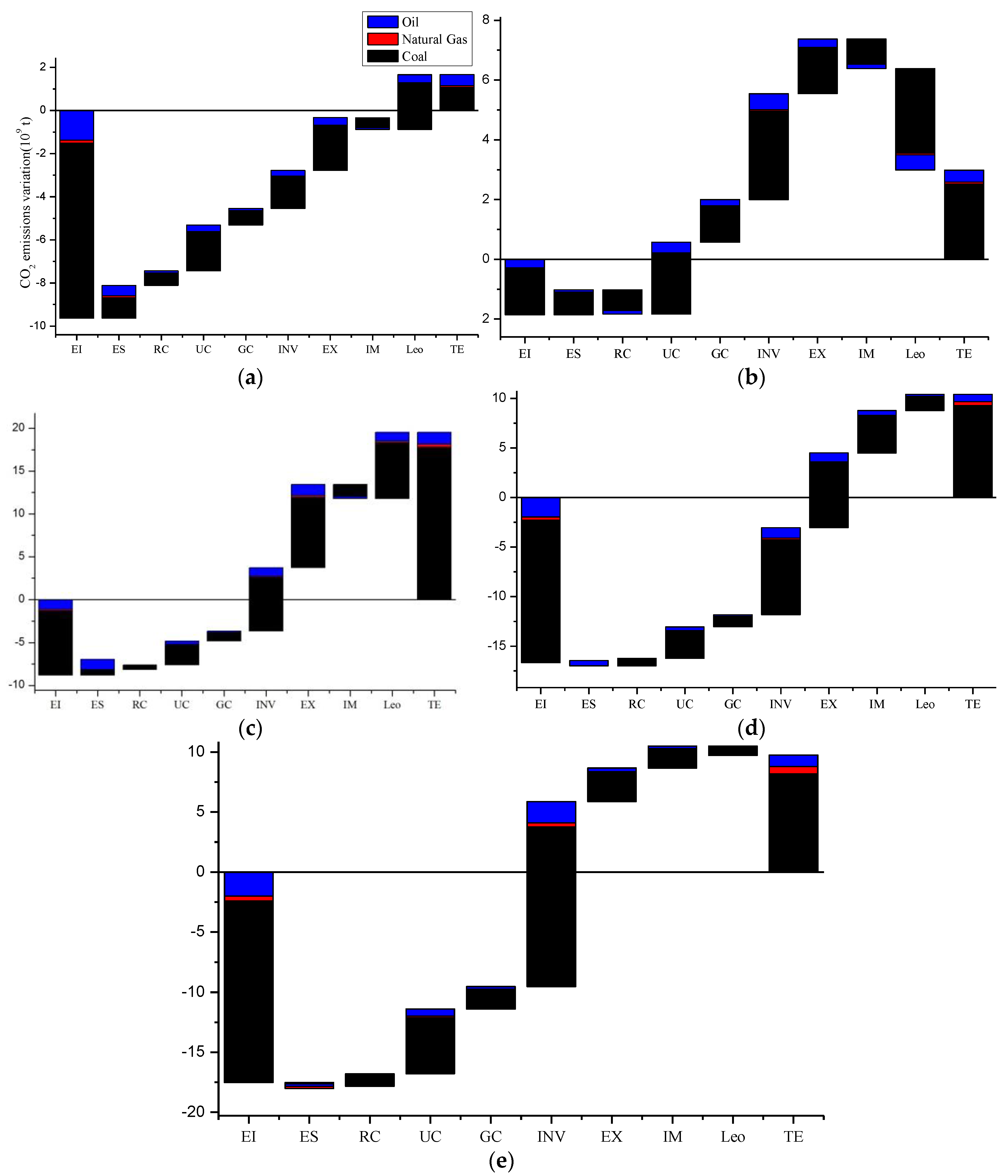
1997–2010	−76.718	2.472	3.208	21.083	8.035	46.263	25.372	0.298	14.326	44.339

shows values for changes in each decomposition factor and the total changes in CO₂ emissions. The energy intensity, energy structure, rural, urban, government consumption, capital formation, export, import and Leontief effects are denoted as EI, ES, RC, UC, GC, INV, EX, IM and Leo, respectively, and the TE represents the total effect of CO₂ emissions.

In all the five calculation periods, the energy intensity effect contributed significantly to carbon emission reduction, except 2000–2002. In the first three periods, the increment of CO₂ emission caused by change of energy structure decreased step by step and energy structure effect gradually changed into negative. In the last two periods, the negative energy structure effect means that the change on energy structure can contribute to carbon emission reduction. Consumption expansion effects are basically all positive. Furthermore, the urban consumption effects considerably outweigh rural and government consumption effects. Investment expansion effect, which denotes capital formation, has a remarkable impact on carbon emission and its influence on carbon emissions is increasingly significant. Compared with energy intensity and final demand effects (RC, UC, GC, and INV), other decomposition factors whose direction of the influence changed over time have less impact on the changes in CO₂ emissions. Eventually, although energy intensity has a great contribution to emission reduction, due to the summation of consumption expansion, capital formation, economic expansion and other factors, the total effects of the five intervals are all positive.

Note that, before the deeper analysis, the validity and rationality of the results in our paper need to be tested. Previous relevant studies are selected to test the rationality of the results. A typical relative research is issued by Su and Ang [46]. They applied LDMI-I method to calculate Non-chaining results (long time slice: 1997–2007) and chaining results (shorter time slice: 1997–2002 and 2002–2007; and 1997–2000, 2000–2002, 2002–2005 and 2005–2007). The overall changes of CO₂ are decomposed into emission intensity effect, Leontief effect and final demand effect. The results in [46] revealed that and the final demand effect is the most important driver to stimulate CO₂ emissions, and change in emission intensity significantly cut emissions. Compared to these two effects, the structure change effect is not significant enough. Take the period 2005–2007 as an example, in Ref. [46], the total CO₂ change, emission intensity, final demand effects are 959.8, −1684.2, and 762.8 million ton of CO₂, and 1041.4, −1666, and 1392 ton of CO₂, respectively, in our research. Obviously, the results in our paper are in line with the results in [46]. Moreover, our research further splits the emission intensity effect into energy intensity and structure effects, and final demand effect into consumption, investment, export and import expansion effects.

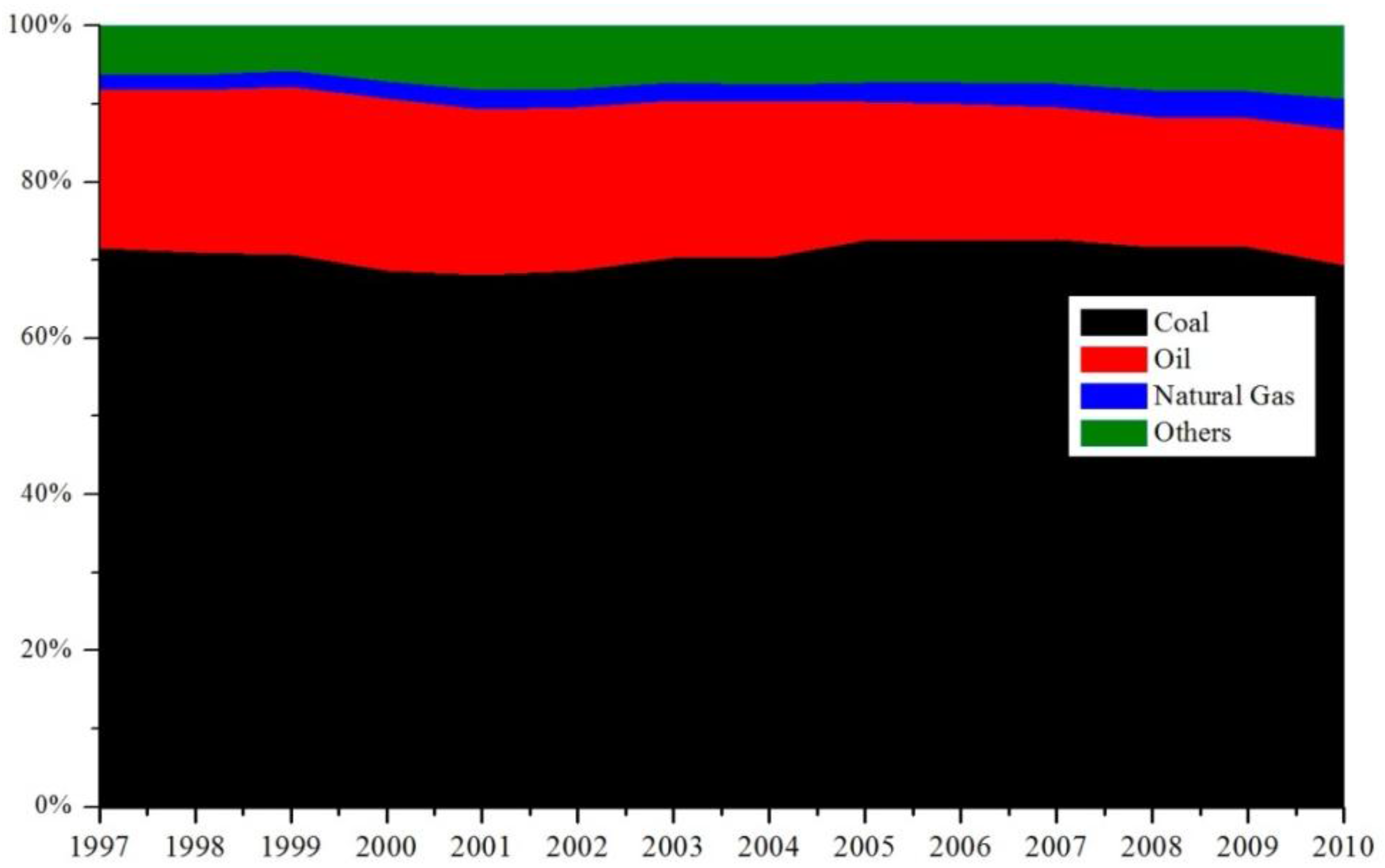
On the basis of Table 5, Figure 1 further demonstrates the influence of these nine decomposition factors on CO₂ emissions changes in the different time intervals more visually. The column length which is composed of three kinds of effects caused by different fossil fuels (coal, oil, and natural gas) refers to the strength of the effect. From an energy perspective, the coal has the most significant contribution in all effects, whether the effects are positive or negative. Secondly, petroleum takes the second part of importance, the effects caused by petroleum can explain about 20% of the total effect. Natural gas, due to the late start of its development and short supply, its effect is very weak compared to the other two, but over time, the effect of natural gas is gradually rising.

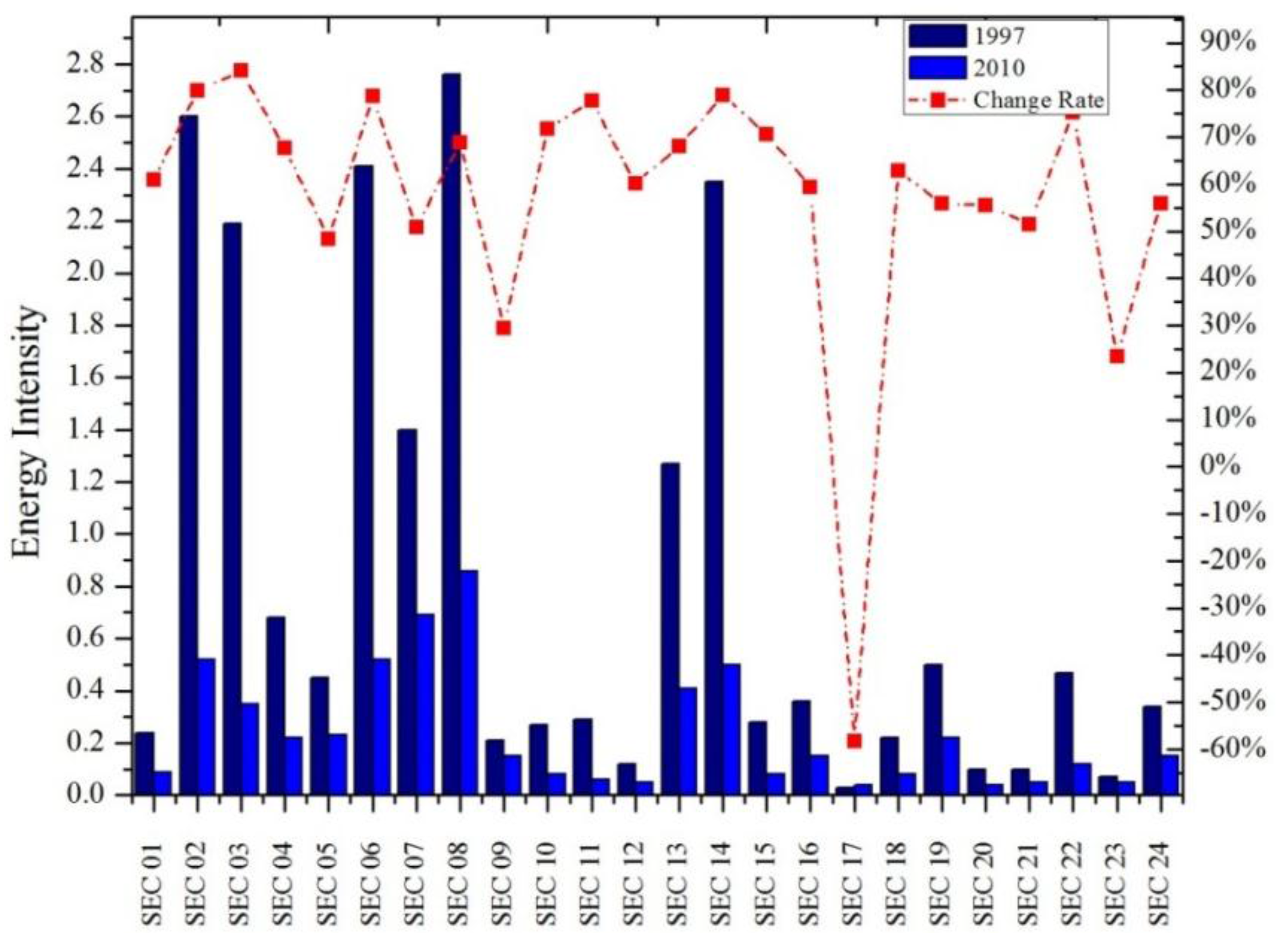
After obtaining the decomposition results in five periods, to analyze driving factors of CO₂ emissions more clearly, we further decompose all the factors into every sector. When considering a particular disaggregation issue, a high level of disaggregation is generally preferred due to the results, which are more refined and representative of what are to be estimated [47]. From a theoretical perspective, the higher disaggregation level can provide more detailed analysis; however, in practice, data availability and the effort required to make further improvement are important in decision-making. There are 24 sectors in

Table 6. Decomposition factors in sub-industries 1997–2010 (Million ton CO₂).

Classification	Sectors	EI	ES	Con	INV	EX	IM	Leo	TE
Agriculture	SEC 01	−165.6	−2.0	30.7	35.5	6.0	−25.5	−44.5	−165.4
Extractive Industry	SEC 02	−560.1	−2.7	4.1	10.3	4.3	−39.6	143.7	−440.0
	SEC 03	−294.7	−1.2	−0.3	5.3	−3.4	−82.8	33.2	−344.0
	SEC 04	−70.3	−0.5	0.0	12.1	2.4	−80.6	74.8	−62.1
	SEC 05	−18.7	−0.3	−0.5	1.1	2.5	−2.7	−57.4	−76.0
Manufacturing Industry (Heavy)	SEC 06	−715.0	−4.0	126.5	−5.4	39.6	62.2	276.9	−219.2
	SEC 07	−420.3	−6.5	−12.3	6.4	91.1	−1.5	−130.2	−473.3
	SEC 08	−1358.3	−15.0	−1.0	103.4	266.7	153.0	364.0	−487.3
	SEC 09	−21.9	−0.8	10.0	12.3	132.3	22.8	−99.7	55.0
	SEC 10	−178.0	−1.2	1.3	667.3	237.4	37.4	−73.1	691.1
	SEC 11	−171.3	−0.9	122.2	627.1	156.5	−12.3	50.7	772.1
	SEC 12	−43.5	−0.5	80.2	347.6	327.4	−3.5	−38.3	669.5
	SEC 13	−827.6	−9.3	102.0	32.7	398.4	25.8	153.8	−124.4
Electricity, Heat and Water	SEC 14	−1110.5	−5.3	212.1	0.0	2.7	−0.5	526.7	−374.9
Manufacturing Industry (Light)	SEC 15	−192.9	−1.5	357.8	12.7	27.0	−0.6	123.1	325.5
	SEC 16	−146.7	−1.7	132.8	5.5	275.4	35.5	−56.1	244.7
	SEC 17	2.9	−0.1	2.4	−5.9	0.5	0.8	−0.4	0.1
	SEC 18	−29.3	−0.3	8.2	29.6	62.3	3.6	12.0	86.2
	SEC 19	−84.6	−1.1	14.4	4.1	50.5	18.7	−50.0	−47.9
	SEC 20	−41.4	−0.5	24.8	292.1	468.0	0.1	34.5	777.6
	SEC 21	−5.0	−0.1	2.6	19.9	79.0	−14.0	8.1	90.5
	SEC 22	−69.7	−0.5	42.3	37.0	33.1	−37.2	−31.4	−26.4
Construction	SEC 23	−23.0	−1.1	42.4	1902.6	32.6	−0.9	−65.9	1886.8
Tertiary Industry	SEC 24	−811.6	−10.0	1630.1	265.2	274.5	−28.3	131.1	1450.8

, with detailed industrial sectors and highly aggregated tertiary industries. Due to the low carbon intensity, some tertiary sectors including financial industry, education and public services merely contribute to CO₂ emissions. Hence, the tertiary sectors are bundled together in this paper. The highly aggregated sectors may lead to a negligence of trade-offs between sectors especially the CO₂ increment caused by trade-offs in sector aggregation. 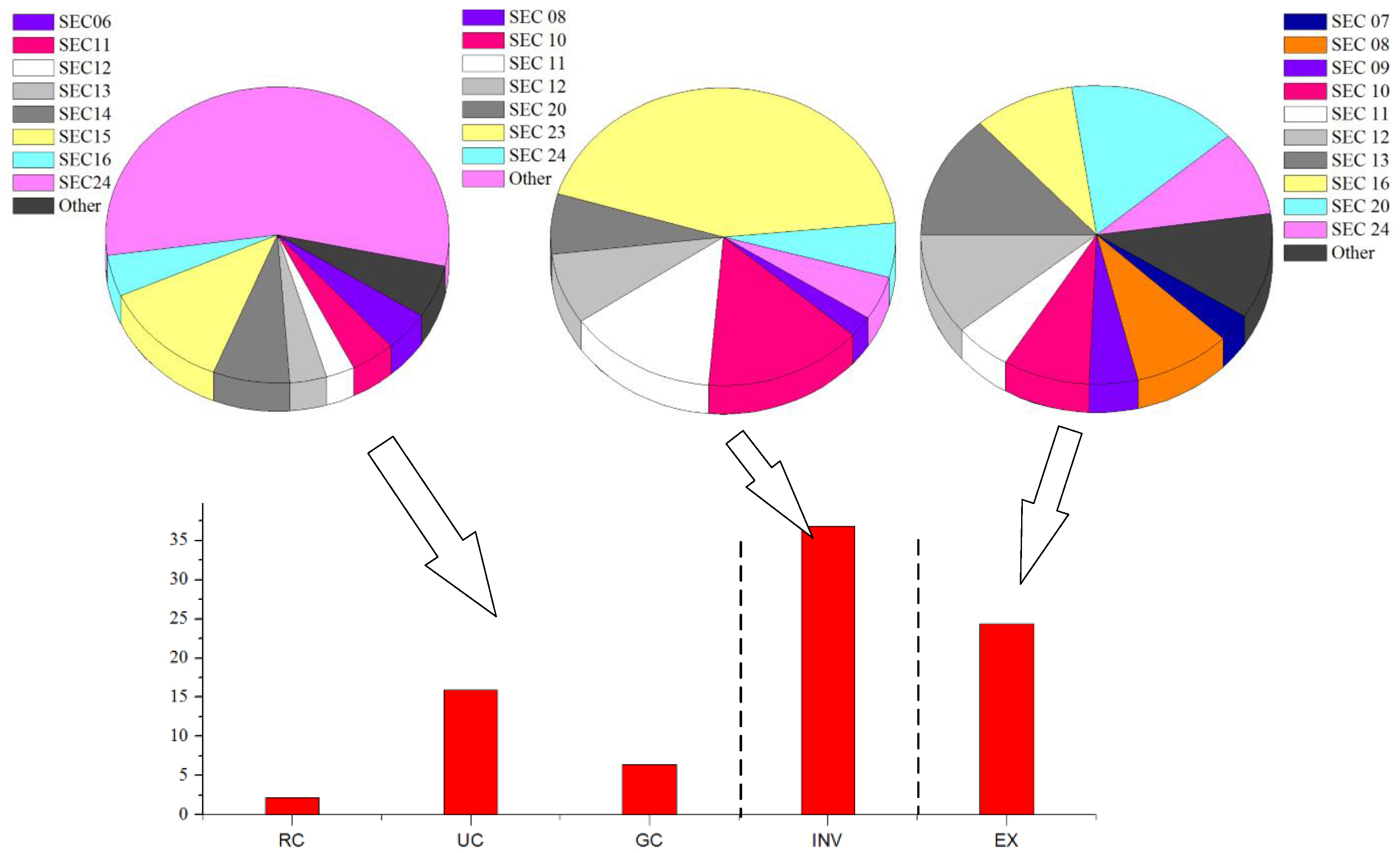Table 6 displays the results of decomposition at sectoral level. The results show that heavy industry, including extractive, manufacturing and electricity, and heat and water industries, plays a decisive role in CO₂ emissions. The energy intensity effects in heavy industry contribute to emission reduction by a large margin. As the branches of heavy industry, extractive industry and electricity and heat and water contribute to 922 and 375 million ton of CO₂ cuts, respectively, whereas the manufacturing industry induces an increase of 883.5 million ton of CO₂. Finally, the heavy industry totally contributes 413.5 million ton of CO₂ emission reductions. Inversely, light industry, construction and tertiary industry greatly promote CO₂ emissions, and they bring about 1450, 1887, and 1451 million ton of CO₂ emissions, respectively. The detailed discussions on all the effects will be stated in the following chapter.

4. Further Discussion

4.1. Energy Intensity Effect

The influence of the variation of energy intensity on change of CO₂ emissions is shown in Figure 1. From 1997 to 2010, the accumulation of CO₂ emission reduction reached 5446 million tons of CO₂. Among them, it reduced CO₂ emissions by 962, 186, 879, 1666 and 1752 million tons in the five periods, respectively.

Figure 2 displays the energy intensities of 24 sectors in 1997 and 2010 with the red line representing change rates. The average drop of energy intensity is nearly 57% in all sectors. Thus, the effect of energy intensity, especially the decline of energy intensity in energy-intensive sectors, is the only one of many utilities that can significantly constrain the CO₂ emissions. It is not peculiar to obtain this result. The emissions of CO₂ mainly derive from the use of fossil energies. In a nutshell, energy utilization is the essence of CO₂ emissions. The heavy industry denotes those industries that provide material bases for all department of national economy. The tag of “energy-intensive” is branded deeply, and sometimes this is indeed the case. In other words, heavy industries have lower energy efficiency and use a large amount of energy in early years. That is why the energy intensity effect can lead to a significant emission-reducing effect. Our results can be perfectly verified by the results of decomposition factors in sub-industries in Table 6. The energy intensity effect in heavy industry far surpassed other sectors and contributed to nearly 80% emission reduction of total energy intensity effect. Then, due to the characteristic of non-energy-intensive, the light industry, tertiary industry, agriculture and construction only contributed to 20% of emission reduction. Furthermore, the total effects of CO₂ are further decomposed into three kinds of fossil fuels. It is shown in Figure 2 that 85% emission-reducing effect in energy intensity effect can be owed to the effect of coal.

An abnormal condition appeared in 2002–2005. There is a nearly sevenfold increase in total effect from period 2000–2002. Compared with previous research that suggested the energy intensity in China experienced an “inflection point” in period 2002–2005, our research shows that China’s overall energy intensity keeps falling during the selected study period. The main reasons are not the sharp increase in energy intensity, but come from Leontief coefficients effect.

4.2. Energy Structure Effect

In the early days, the proportion of coal experienced an increase from 70.7% in 1978 to highest peak of 76.2% in 1986. Soon afterwards, with the eased domestic energy market of supply and demand situation of tension, the share of the coal in primary energy consumption has dropped continually. The lowest proportion 68.5% occurred in 2002. Recent years, the booming energy consumption caused by the rapid economic development resulted in the rise of the coal proportion again. Meanwhile, oil, serving as the second-largest fossil fuel, also plays a pivotal role. From the late 1990s to the beginning of the 21st century, the expansion of China’s foreign trade in oil has caused an increase from 16.6% in 1990 to highest peak of 24% in 2002. Along with the great upheavals of the international situation from 21st century, the oil supply fell short of demand dramatically. In this period, the proportion of domestic oil consumption has declined from 24% to 19% in 2010. Of the various fossil energy sources, natural gas is the only clean energy in fossil fuels. The consumption of natural gas has showed an appreciable increase in recent years. According to “National Plan on Climate Change (2014–2020)”, China’s natural gas consumption in the proportion of primary energy consumption will account for more than 10%. Other energy such as nuclear, hydraulic, wind, and solar power, has been a center of focus. It experienced vigorous growth and doubled over 1990–2010. The rapid development of clean energy has contributed substantially to CO₂ reductions. Figure 3 depicts the variation of China’s energy consumption structure in 1997–2010.

The energy structure effects are shown in Table 5. It is shown that the energy structure effects in the five time periods are 152, 84, 64, −32, and −67 million tons, respectively. The heavy industry, especially manufacturing industry, is mostly low-use, high pollution and high consumption of the extensive economic growth mode, and this situation is particularly serious in China and especially in early years. China’s energy consumption has more than doubled in period 1997–2010. In early stage, the Chinese government has been pursuing the rapid economic development, ignoring the environmental problems. The unreasonable energy structure and energy waste contributed to the increase of the CO₂ emissions in 1997–2000, 2000–2002 and 2002–2005. However, the blind pursuit of economic growth, the narrow concept of development has begun to expose its inherent defects that the ecological environment of human life cannot bear sustained and rapid growth. The Chinese government gradually put emphasis on the energy structure adjustment. With speed up of China’s energy structure adjustment, the proportion of clean energy in terminal energy continued to increase. Eventually, the energy structure effects turn to negative step by step, which means that the energy structure is shifting to low carbon, and tends to be more reasonable.

4.3. Final Demand Effect

The final demand structure contains consumption (rural, urban and government), capital formation and net export. It is well known that Chinese economic development heavily relies on investment, consumption and export, which are called “troika”. Table 5 and Table 6 reveal that the final demand structure is the most important driving factor for the growth of China’s CO₂ emissions from 1997 to 2010. Moreover, to obtain a more in-depth analysis, we further decompose the final demand effect to every sector. The results are shown in Figure 4.

4.3.1. Consumption Expansion Effect

Consumption, especially urban consumption, greatly boosted the CO₂ emissions. The results in Table 5 show a significant trend for an increase in urban consumption expansion effects. With the acceleration of urbanization, urban consumption, from 1.8 trillion in 1997 to 11.2 trillion in 2010, increased by more than six times in 13 years. Compared to the urban residents, the income level of rural residents in China remained relatively low level. The government consumption also increased by six times, but merely concentrated in the third industry. Hence, both rural and government consumption effects on boosting carbon emissions are weaker. Meanwhile, the great increases in consumption result in the sharp increase of CO₂ in most sectors. Figure 4 demonstrates that the contribution degree of service, foods and textile reached 55.6%, 12.2% and 4.6%, respectively. Moreover, the electricity and heat power, petroleum and transport equipment also contributed 7.3%, 4.3%, and 4.2%, respectively. Take the service industry as an example. Although most of tertiary industries are low and even zero emission such as finance, education, etc., the consumption expansion effect can also lead to a sharp rise in CO₂ emissions, which is mainly due to the sub-sectors such as transportation, warehousing and postal service are closely related to carbon emissions. Moreover, the linkage effect between industries can also contribute significantly to CO₂ emissions. For instance, the demands of private transportation can drive the transport equipment industry and complementary goods such as petroleum. Undoubtedly, the surge in consumption in these typical sectors has sent CO₂ emissions skyrocketing.

4.3.2. Investment Expansion Effect

Investment serves as the “troika” of the economic growth, has always made a significant contribution on CO₂ growth. The pie chart in the middle in Figure 4 shows that seven sectors contribute significantly to CO₂ emissions growth in the process of capital formation. Among them, 43.8% of increment causes by capital formation of construction. Historically, the added value of construction reached 1898 billion Yuan in 2010, more than septupled since 1997. Along with urbanized and modernized advancement quickening, more and more municipal construction and other facilities have been launched by the government. In recent years, the growth of FAI (total fixed asset investment) maintained a high level. Following the construction, the manufacturing industry, including manufacture of special and general purpose machinery, transport equipment, electrical equipment, and electronic equipment, occupied second place. Although manufacturing is developing rapidly with significant investment needs, it is nowhere near the construction industry. Three heavy industries, SEC 10, SEC 11, and SEC 12, and one light industry, SEC 20, contributed 15%, 14%, 7.8% and 6.5% increment of CO₂ emissions, respectively. In recent years, the manufacturing growth is significantly faster than the overall growth of the national economy, which largely promoted the CO₂ emissions. Furthermore, the results in Table 6 perfectly demonstrated that the investment expansion effects are mainly concentrated in heavy industry and construction. Other sectors, containing the agriculture, most of light industries and extractive industry, metal and nonmetal ores and so on, merely contributed 4.76% increment of CO₂ emissions in the process of capital formation.

4.3.3. Export Expansion and Import Substitution Effect

In this part, export expansion and import substitution effects or (net export effect) are specified. The analysis of carbon emissions from China’s import and export trade shows that China is a country with net exporter of embodied carbon emissions in whole calculation period 1997–2010. Due to the foreign trade, China saved 2144 million ton of CO₂ for foreign countries, which accounted for about 48% of total CO₂ increment. The right pie chart in Figure 4 demonstrates that nearly 90% of carbon emission increments caused by export expansion effect come from industrial sectors, among which there is an equal split of heavy industry and light industry. Determined by China’s national conditions, Chinese enterprises are located in the bottom of the global value chain, and undertake the process of manufacturing with large energy consuming and high carbon emission. Most of manufacturing industries, particularly electronics, transportation and other equipment manufacturing industries which have comparatively big exporting amount undertaking large amount environmental costs for foreign countries. In addition, the tertiary industry led to a 9.3% increase in carbon emission. China’s trade in services is supported by traditional tourism and transportation industries, which belong to resource and labor intensive industry, whereas capital intensive services such as aviation, communications and architecture as well as knowledge intensive services, such as financial, computer and information services, contribute to trade in service weakly.

4.4. Leontief Effect

In the whole economy, labor and capital are not merely consumed in final demand and consumption but also in the intermediate outputs. Leontief effects (also called intermediate demand effect) contribute to 254, −340, 776, 163 and −76 million tons of CO₂, respectively, as seen in Table 5. It seems that the effect is not stable enough and not in conformity with the trend of economic fluctuations. Previous research revealed that the main reason for the total output growth is the rise in final demand, while the effect of Leontief inverse matrix is not stable [28,48,49]. The abnormal condition appeared in 2002–2005 as we mentioned above. The Leontief effect leaped from −340 to 776 million ton of CO₂. In 2002, although the government vigorously promoted energy conservation and emission reduction policies, a new round of economic growth dominated by heavy chemical industry resulted in the upsurge of CO₂ emissions. During this period, the unreasonable changes on industrial structure accompanied with the stagnation of technological progress become the main causes of carbon increment. Although the short term Leontief effects fluctuate greatly, the total Leontief effect in 1997–2010 reveals that it can significantly contribute to CO₂ emissions. To dig deeply into the inherent reasons, we commence from the angle of the industry. The average influence coefficients are shown in

Table 7. The average influence coefficients in all sectors from 1997 to 2010.

Sectors	Coefficient	Sectors	Coefficient	Sectors	Coefficient	Sectors	Coefficient
SEC 01	0.69	SEC 07	0.92	SEC 13	1.09	SEC 19	1.05
SEC 02	1.02	SEC 08	1.13	SEC 14	1.06	SEC 20	1.07
SEC 03	0.66	SEC 09	1.16	SEC 15	1.08	SEC 21	1.17
SEC 04	0.95	SEC 10	1.11	SEC 16	0.91	SEC 22	0.83
SEC 05	0.90	SEC 11	1.18	SEC 17	1.04	SEC 23	0.92
SEC 06	1.02	SEC 12	1.19	SEC 18	1.07	SEC 24	0.78

.

The significant positive Leontief effects mainly appear in SEC 02, SEC 06, SEC 08, SEC 13, SEC 14, SEC 15, and SEC 24, most of whose influence coefficient is greater than 1. When the influence coefficient is greater than 1, it indicates that this sector has a bigger pulling effect of domestic demand. In other word, an “Amplification Effect” will appear in these sectors. As long as there is a demand, whether it is investment, consumption or others, the effect will be magnified. The amplified effect will further promote the demands of various sectors of the national economy and conversely foster greater intermediate inputs. Eventually, this series of chain reactions will collaboratively decide a positive effect on CO₂ emissions due to demand expansion.

5. Conclusions and Policy Implications

This paper tries to investigate driving forces of changes in CO₂ emissions in China. The drivers of carbon emissions growth are further decomposed into nine sub-effects. The results of this paper indicate that the energy intensity effect is the most predominant driving force to stimulate emission mitigation. Compared to energy intensity effect, the energy structure effects turn to negative step by step, which means that the energy structure is shifting to low carbon, and tends to be more reasonable. To simplify the expression, rural, urban and government consumption are bundled up. The urban consumption predominantly overwhelmed the other two and greatly boosts the CO₂ emissions. Among the final demand effect, the investment and export expansion are the two biggest contributors to increment of CO₂ emissions. The investment expansion effect has always made a significant contribution on CO₂ growth, among which 43.8% of increment effect of CO₂ caused by capital formation of construction. In addition, the analysis of carbon emissions from China’s import and export trade shows that China is a country with net exporter of embodied carbon emissions in 1997–2010 and nearly 90% of CO₂ emission increments come from industrial sectors. Although the short term Leontief effect is not in conformity with the trend of economic fluctuations, the total Leontief effect in 1997–2010 reveals that it can significantly contribute to CO₂ emissions. The deeper analyses show that those industries whose influence coefficients are greater than 1 have “Amplification Effect” and result in a positive Leontief effect in general.

The above conclusions theoretically provide vital information to shape policy schemes for reducing CO₂ emissions. However, the deep analysis of policy implications for Chinese government is necessary. Hence, some policy implications for cutting the consumption of high-carbon energy and embodied carton emissions in export are as follows.

“Green policy” is an effective approach to cut CO₂ emissions and consumption of high-carbon energy. There are two main types of emission reduction policies prevailed abroad: carbon tax policy and Emission Trading Scheme (ETS). The former one is a mandatory policy that is characterized by price control, and the latter one is a market-based policy that is characterized by the total amount control. Despite the different mechanism of these two kinds of policies, both of them influence the market elements by price leverage. In a nutshell, both of them can lower market competitiveness of fossil fuels by raising their cost of use. Additionally, accelerating the upgrade of the structure of export commodities and optimizing the trade mix can reduce embodied carbon emissions in export effectively. From the perspective of China’s export structure, CO₂ intensive products constitute a large proportion. The current international trade in China still stagnates in a net exporter of embodied carbon emissions. To prevent China from becoming “Pollution haven”, the cut of export rebate rate and the change for the policy of export rebate seems to be an effective way. In the meantime, strengthening the international competitiveness of non-energy intensive sectors, such as the service sectors, the wholesale and retail sectors, is another effective method to optimize export structure and reduce embodied carbon emissions in export.

References

1. Lovett, J.C.; Hofman, P.S.; Morsink, K.; Torres, A.B.; Clancy, J.S.; Krabbendam, K. Review of the 2008 UNFCCC meeting in Poznań. Energy Policy 2009, 37, 3701–3705. [Google Scholar] [CrossRef]
2. Francesch-Huidobro, M. Climate change and energy policies in Shanghai: A multilevel governance perspective. Appl. Energy 2016, 164, 45–56. [Google Scholar] [CrossRef]
3. Specht, E.; Redemann, T.; Lorenz, N. Simplified mathematical model for calculating global warming through anthropogenic CO2. Int. J. Therm. Sci. 2016, 102, 1–8. [Google Scholar] [CrossRef]
4. Xiao, H.; Wei, Q.; Wang, H. Marginal abatement cost and carbon reduction potential outlook of key energy efficiency technologies in China’s building sector to 2030. Energy Policy 2014, 69, 92–105. [Google Scholar] [CrossRef]
5. Isard, W.; Bassett, K.; Choguill, C.; Furtado, J.; Izumita, R.; Kissin, J.; Romanoff, E.; Seyfarth, R.; Seyfarth, R.; Tatlock, R. On the Linkage of Socio-Economic and Ecologic Systems. Pap. Reg. Sci. Assoc. 1968, 21, 79–99. [Google Scholar] [CrossRef]
6. Leontief, W. Environmental repercussions and the economic structure: An input–output approach. Rev. Econom. Stat. 1970, 52, 262–271. [Google Scholar] [CrossRef]
7. Zou, Q.; Liu, X. Economic effects analysis of seawater desalination in China with input–output technology. Desalination 2016, 380, 18–28. [Google Scholar] [CrossRef]
8. Song, J.; Yang, W.; Zhao, L.; Higano, Y.; Wang, X. Discovering the energy, economic and environmental potentials of urban wastes: An input–output model for a metropolis case. Energy Convers. Manag. 2016, 114, 168–179. [Google Scholar] [CrossRef]
9. Cortés-Borda, D.; Guillén-Gosálbez, G.; Jiménez, L. Assessment of nuclear energy embodied in international trade following a world multi-regional input–output approach. Energy 2015, 91, 91–101. [Google Scholar] [CrossRef]
10. Marcucci, A.; Fragkos, P. Drivers of regional decarbonization through 2100: A multi-model decomposition analysis. Energy Econ. 2015, 51, 111–124. [Google Scholar] [CrossRef]
11. Shahiduzzaman, M.; Layton, A. Decomposition analysis to examine Australia’s 2030 GHGs emissions target: How hard will it be to achieve? Econ. Anal. Policy 2015, 48, 25–34. [Google Scholar] [CrossRef]
12. Moutinho, V.; Moreira, A.C.; Silva, P.M. The driving forces of change in energy-related CO2 emissions in Eastern, Western, Northern and Southern Europe: The LMDI approach to decomposition analysis. Renew. Sustain. Energy Rev. 2015, 50, 1485–1499. [Google Scholar] [CrossRef]
13. Lu, Z.; Yang, Y.; Wang, J. Factor Decomposition of Carbon Productivity Chang in China’s Main Industries: Based on the Laspeyres Decomposition Method. Energy Procedia 2014, 61, 1893–1896. [Google Scholar]
14. Liu, F.L.; Ang, B.W. Eight methods for decomposing the aggregate energy-intensity of industry. Appl. Energy 2003, 76, 15–23. [Google Scholar] [CrossRef]
15. Ang, B.W. The LMDI approach to decomposition analysis: A practical guide. Energy Policy 2005, 33, 867–871. [Google Scholar] [CrossRef]
16. Ang, B.W. Decomposition analysis for policymaking in energy: Which is the preferred method? Energy Policy 2004, 32, 1131–1139. [Google Scholar] [CrossRef]
17. Ang, B.W. LMDI decomposition approach: A guide for implementation. Energy Policy 2015, 86, 233–238. [Google Scholar] [CrossRef]
18. Su, B.; Ang, B.W. Structural decomposition analysis applied to energy and emissions: Some methodological developments. Energy Econ. 2012, 34, 177–188. [Google Scholar] [CrossRef]
19. Betts, J.R. Two exact, non-arbitrary and general methods of decomposition temporal change. Econ. Lett. 1989, 30, 151–156. [Google Scholar] [CrossRef]
20. Dietzenbacher, E.; Los, B. Structural decomposition techniques: Sense and sensitivity. Econ. Syst. Res. 1998, 10, 307–323. [Google Scholar] [CrossRef]
21. Hoekstra, R.; van der Bergh, J.C.J.M. Comparing structural and index decomposition analysis. Energy Econ. 2003, 25, 39–64. [Google Scholar] [CrossRef]
22. Xu, Y.; Dietzenbacher, E. A structural decomposition analysis of the emissions embodied in trade. Ecol. Econ. 2014, 101, 10–20. [Google Scholar] [CrossRef]
23. Cellura, M.; Longo, S.; Mistretta, M. Application of the Structural Decomposition Analysis to assess the indirect energy consumption and air emission changes related to Italian households consumption. Renew. Sustain. Energy Rev. 2012, 16, 1135–1145. [Google Scholar] [CrossRef]
24. Cansino, J.M.; Román, R.; Ordóñez, M. Main drivers of changes in CO2 emissions in the Spanish economy: A structural decomposition analysis. Energy Policy 2016, 89, 150–159. [Google Scholar] [CrossRef]
25. Kopidou, D.; Tsakanikas, A.; Diakoulaki, D. Common trends and drivers of CO2 emissions and employment: A decomposition analysis in the industrial sector of selected European Union countries. J. Clean. Prod. 2016, 112, 4159–4172. [Google Scholar] [CrossRef]
26. Wachsmann, U.; Wood, R.; Lenzen, M.; Schaeffer, R. Structural decomposition of energy use in Brazil from 1970 to 1996. Appl. Energy 2009, 86, 578–587. [Google Scholar] [CrossRef]
27. Lan, J.; Malik, A.; Lenzen, M.; McBain, D.; Kanemoto, K. A structural decomposition analysis of global energy footprints. Appl. Energy 2016, 163, 436–451. [Google Scholar] [CrossRef]
28. Lin, B.; Xie, X. CO2 emissions of China’s food industry: An input–output approach. J. Clean. Prod. 2016, 112, 1410–1421. [Google Scholar] [CrossRef]
29. Yuan, R.; Zhao, T. Changes in CO2 emissions from China’s energy-intensive industries: A subsystem input-output decomposition analysis. J. Clean. Prod. 2016, 117, 98–109. [Google Scholar] [CrossRef]
30. Zhang, H.; Lahr, M.L. China’s energy consumption change from 1987 to 2007: A multi-regional structural decomposition analysis. Energy Policy 2014, 67, 682–693. [Google Scholar] [CrossRef]
31. Li, F.; Song, Z.; Liu, W. China’s energy consumption under the global economic crisis: Decomposition and sectoral analysis. Energy Policy 2014, 64, 193–202. [Google Scholar] [CrossRef]
32. Xie, S.C. The driving forces of China’s energy use from 1992 to 2010: An empirical study of input–output and structural decomposition analysis. Energy Policy 2014, 73, 401–415. [Google Scholar] [CrossRef]
33. Tarancon, M.A.; Río, P.D. Assessing energy-related CO2 emissions with sensitivity analysis and input–output techniques. Energy 2012, 37, 161–170. [Google Scholar] [CrossRef]
34. Wang, F.; Dong, B.; Yin, X.; An, C. China’s structural change: A new SDA model. Econ. Model. 2014, 43, 256–266. [Google Scholar] [CrossRef]
35. Yang, L.; Lahr, M.L. Sources of Chinese labor productivity growth: A structural decomposition analysis, 1987–2005. China Econ. Rev. 2010, 21, 557–570. [Google Scholar] [CrossRef]
36. Yang, Z.; Liu, H.; Xu, X.; Yang, T. Applying the Water Footprint and dynamic Structural Decomposition Analysis on the growing water use in China during 1997–2007. Ecol. Indic. 2016, 60, 634–643. [Google Scholar] [CrossRef]
37. Xia, Y.; Yang, C.H.; Chen, X.K. Structural decomposition analysis on China’s energy intensity Change for 1987–2005. J. Syst. Sci. Complex. 2012, 15, 156–166. [Google Scholar] [CrossRef]
38. Zeng, L.; Xu, M.; Liang, S.; Zeng, S.; Zhang, T. Revisiting drivers of energy intensity in China during 1997–2007: A structural decomposition analysis. Energy Policy 2014, 67, 640–647. [Google Scholar] [CrossRef]
39. Liu, X. Some theoretical problems in the application of constant price input-output table. J. Stat. Decis. Mak. 2011, 18, 12–16. (In Chinese) [Google Scholar]
40. National Bureau of Statistics of China. China Statistical Yearbook 2015; China Statistics Press: Beijing, China, 2015.
41. National Bureau of Statistics of China. China Energy Statistical Yearbook 2014; China Statistics Press: Beijing, China, 2014.
42. State Environmental Protection Administration, State Information Center. Analysis and Forecast of China's Environmental Economic Situation; China Environmental Science Press: Beijing, China, 2008. [Google Scholar]
43. Su, B.; Ang, B.W. Input–output analysis of CO2 emissions embodied in trade: Competitive versus non-competitive imports. Energy Policy 2013, 56, 83–87. [Google Scholar] [CrossRef]
44. Weber, C.L.; Peters, G.P.; Guan, D.; Hubacek, K. The contribution of Chinese exports to climate change. Energy Policy 2008, 36, 3572–3577. [Google Scholar] [CrossRef]
45. Lin, B.; Sun, C. Evaluating carbon dioxide emissions in international trade of China. Energy Policy 2010, 38, 613–621. [Google Scholar] [CrossRef]
46. Su, B.; Ang, B.W. Structural decomposition analysis applied to energy and emissions: Aggregation issues. Econ. Syst. Res. 2012, 24, 299–317. [Google Scholar] [CrossRef]
47. Su, B.; Huang, H.C.; Ang, B.W.; Zhou, P. Input–output analysis of CO2 emissions embodied in trade: The effects of sector aggregation. Energy Econ. 2010, 32, 166–175. [Google Scholar] [CrossRef]
48. Afrasiabi, A.; Casler, S. Product mix and technological change within the Leontief inverse. J. Reg. Sci. 1991, 31, 147–160. [Google Scholar] [CrossRef]
49. Nie, H. Research on the Problems and Solutions for the Increase of Energy Consumption in China. Ph.D. Thesis, Jilin University, Changchun, China, December 2013. [Google Scholar]
Figure 1. Contribution of different effects on CO2 emissions changes in China. (a) changes in CO2 emissions in 1997–2000; (b) changes in CO2 emissions in 2000–2002; (c) changes in CO2 emissions in 2002–2005; (d) changes in CO2 emissions in 2005–2007; (e) changes in CO2 emissions in 2007–2010.
Energies 09 00259 g001
Figure 2. The energy intensities of 24 sectors.
Energies 09 00259 g002
Figure 3. The energy structure in 1997–2010.
Energies 09 00259 g003
Figure 4. The contribution of different end uses on CO2 emissions growth.
Energies 09 00259 g004