Market Suitability and Performance Tradeoffs Offered by Commercial Wind Turbines across Differing Wind Regimes ^†

Abstract

The suitability of turbine configurations to different wind resources has been traditionally restricted to considering turbines operating as standalone entities. In this paper, a framework is thus developed to investigate turbine suitability in terms of the minimum cost of energy offered when operating as a group of optimally-micro-sited turbines. The four major steps include: (i) characterizing the geographical variation of wind regimes in the onshore U.S. market; (ii) determining the best performing turbines for different wind regimes through wind farm layout optimization; (iii) developing a metric to quantify the expected market suitability of available turbine configurations; and (iv) exploring the best tradeoffs between the cost and capacity factor yielded by these turbines. One hundred thirty one types of commercial turbines offered by major global manufacturers in 2012 are considered for selection. It is found that, in general, higher rated power turbines with medium tower heights are the most favored. Interestingly, further analysis showed that “rotor diameter/hub height” ratios greater than 1.1 are the least attractive for any of the wind classes. It is also observed that although the “cost-capacity factor” tradeoff curve expectedly shifted towards higher capacity factors with increasing wind class, the trend of the tradeoff curve remained practically similar.

1. Introduction

1.1. A Temporally- and Spatially-Varying Energy Resource

The intermittency of a wind resource at a location and the variation of the wind pattern from one location to another present significant challenges to advancing the penetration of wind energy. Appreciable work has been done (and is ongoing) (i) to account for the variation of wind conditions at a particular site (e.g., wind distribution modeling [1,2]) and (ii) to address the intermittency of wind resources in the context of grid integration (e.g., energy storage technologies [3,4]). In contrast, there has been a limited amount of work that investigates the complex demands on wind turbine performance (when considered as a group) presented by the variety of wind patterns (e.g., different wind classes) existing in the entire market.

The major turbine manufacturers offer a family/series of wind turbines to suit the market needs of different wind regimes. In this context, to promote better decision making both at the level of the turbine manufacturers and the farm developers in different geographical regions, the following explorations are needed: (i) explorative studies that provide a global understanding of the suitability of different turbine feature combinations (e.g., dimensions and power characteristics) for different wind regimes; and (ii) an analysis of the economic and production potential offered by the most suitable turbine configurations (among those commercially available). In this context, it is also important to realize that such explorations need to consider wind turbine performance and the associated cost of energy in the context of their operation as a group of optimally-micro-sited turbines. Under a group operation, as is the case with utility-scale wind farms, individual wind turbines may be subject to a wind class (or wind regime) that is different from the (free flow) wind class of that site owing to wake effects; additionally, true performance and economic potential are only reflected by the operation of a system under an optimized scenario. Stand-alone turbine suitability ratings, such as the IEC rating [5], elude all of the above insights and, thus, provide limited fundamental understanding of turbine suitability under utility-scale deployment.

Therefore, this paper aims: (1) to develop a framework to determine the most suitable turbine configurations for different wind regimes (derived from a wind map), under optimized group operation; (ii) to analyze the cost of energy (COE) offered by the best performing turbines and the market suitability of different turbine feature combinations for the onshore U.S. market; and (iii) to explore the best cost/capacity factor tradeoffs offered by the most suitable turbine feature combinations for different wind classes. In accomplishing these objectives, this paper presents a synergy and extension of the research presented earlier by Chowdhury et al. [6,7]. In this paper, the suitability of turbine-features is studied by considering 131 different configurations available commercially in 2012 from the major global manufacturers. Thus, the explorations of turbine potentials (across various wind regimes) presented in this paper are performed based on existing turbine technologies available in or before 2012. The analysis of emerging turbine technology or turbine design is however not within the scope of this paper. The following three Subsections, Section 1.2, Section 1.3 and Section 1.4, respectively discuss the role of turbine selection in wind farm planning, the observed variation of wind patterns in a national market, and the major components of the exploration framework developed in this paper.

1.2. Role of Turbine Selection in Wind Farm Design

Post wind resource assessment of a site, two of the primary objectives of optimal wind farm planning are to (i) minimize the cost of energy (COE), expressed in $/kWh, and/or (ii) maximize the capacity factor (CF). Successful accomplishment of these objectives demands a robust and flexible wind farm optimization platform that allows appropriate consideration of the following critical factors:

• The installed capacity of the wind farm,
• The land configuration and the placement of turbines in the wind farm (i.e., macro- and micro-siting), and
• The types of wind turbines to be installed.

In this paper, we are particularly concerned with the role of the third factor in wind farm performance. A turbine (or a set of turbines) that offers the most attractive tradeoff between (i) the life cycle costs and (ii) the predicted long-term energy production capacity at a given site can be considered suitable for developing a wind farm at that site.

The long-term energy production capacity of a wind turbine at a particular site depends on the expected distribution of wind conditions (mainly wind speed) at that site. Taking a more gross wind strength perspective of a given site, this allows classifying turbines based on their suitability to sites in terms of an annual (long-term) average wind speed rating. The average wind speed rating for a turbine is generally provided by the manufacturer as a component of the specified IEC Wind Turbine Class rating [5]. However, considering that each turbine operates as a part of an entire array in a commercial wind farm, the relation of its power generation performance to its average wind speed rating is seldom straightforward. In quantifying the energy production capacity of a farm, it is important to recognize and account for the wake-induced interactions among the turbines in the farm. To this end, an optimal wind farm design process should simultaneously consider the farm layout and the turbine type selection [8]. Another important criterion for turbine selection is its load-bearing capacity. In this context, the IEC wind turbine rating provides the compatibility of the turbine with respect to standard turbulence intensity measures. The determination of the local average wind gusts at a site and the subsequent turbulence intensity measures is a crucial part of wind resource assessment. However, such information is site specific, and long-term turbulence intensity maps for an entire region are generally not available. Hence, the load-bearing capacity of turbines is not considered as a compatibility criterion in this paper.

In this paper, we focus on the following two important aspects of a turbine to determine its geographical compatibility.

• Actual energy production capacity of a turbine (when operating as a group) based on the local wind resource, and
• Leveled cost of the wind farm attributable to the turbines.

In this context, commercially-available wind turbines are defined in terms of five major features: (i) rated power, (ii) power characteristics, (iii) rotor-diameter, (iv) hub-height and (v) drive-train type.

The decision making regarding the placement of turbines and the type(s) of turbines to be installed are interdependent, and should ideally be performed simultaneously when designing optimal wind farm configurations. To this end, the unrestricted wind farm layout optimization (UWFLO), an advanced wind farm design method developed in [8,9], is adopted in this paper, particularly due to its capability to simultaneously optimize the selection and siting of turbines. There are very few other methods that also account for aspects of turbine selection in tandem with turbine placement; one other example includes the method presented by Chen et al. [10], which considers differing hub-heights as an optimization parameter in maximizing wind farm power output. Other powerful wind farm layout optimization methods include those developed in [11,12,13,14,15,16,17,18,19]. The majority of these methods, while providing important and diverse capabilities in the context of turbine micro-siting for a single wind farm, do not simultaneously focus turbine type selection during the layout optimization process, as is required in the explorations presented in this paper.

1.3. Geographical Variation of Wind Patterns

The performance of a wind farm is regulated by the nature of the resource at the site. Turbines of varying types are suitable for different wind patterns, and this necessitates the appropriate classification and representation of wind patterns. The National Renewable Energy Laboratory (NREL) distinguishes seven classes of wind patterns, based on their estimated average wind speed (AWS) and wind power density (WPD) [20]. Each wind class in the NREL seven-class system spans two values of mean wind speed and two associated values of wind power density. The mean wind speed, derived from the Rayleigh distribution, corresponds to an equivalent mean wind power density [20]. These two metrics, the mean wind speed and the WPD values, can be regarded as measures of the resource strength of a wind site. The values of the different mean/average wind speeds that are experienced across a region are often available in the form of wind maps (e.g., the U.S. wind map [21]). However, the ranges of AWS need not be restricted to just seven wind classes; in fact, a finer variation of wind patterns/regimes is desirable when exploring turbines suitable for different wind patterns.

Appropriate representation of the wind pattern variations over an entire wind energy market area is therefore the first step toward understanding “turbine to operating-conditions” compatibility. In this paper, the compatibility of a turbine is defined by its likelihood to be selected during wind farm layout optimization, where the objective is to minimize the wind farm’s energy costs. In order to quantify the annual energy production (AEP) for a candidate wind farm design, information regarding the local long-term variation of wind conditions is required. In this paper, the long-term AWS is used to represent a wind resource, which has the following two advantages: (i) a one-parameter distribution of wind speed can be readily derived from the AWS to represent the approximate variation of wind conditions at the concerned site; and (ii) the resource strength of the site can be readily related to a wind map that represents the wind resources over a region in terms of their estimated AWS. In the context of the first advantage (stated above), it is important to note that both the Weibull and Rayleigh distribution are known to provide an acceptable description of wind speed probability [22,23,24,25] (although the former is more popular and, in general, more accurate). The Rayleigh distribution is a one-parameter model, and we exploit this characteristic to derive an approximate wind speed distribution from the “average wind speed” information; where a unique value of the distribution parameter can be determined from a given value of the mean of the distribution.

1.4. Exploring “Turbine-Wind Regime” Compatibilities

The determination of suitable commercial-scale turbines and their optimal placement for a given resource is itself a complex process. The determination of suitable commercial turbine types and their likely demand in an entire target market with different wind regimes is therefore a challenging task; to the best of the authors’ knowledge, such an exploration is rare in the literature. To accomplish this challenging task, this paper develops a comprehensive framework that comprises the following four steps:

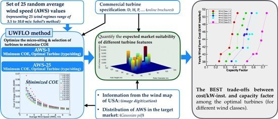
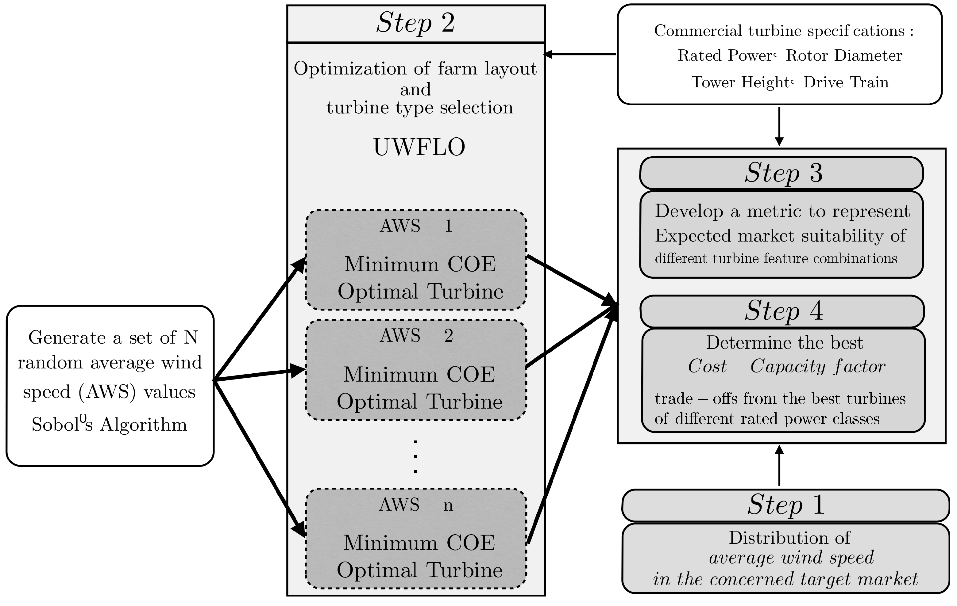
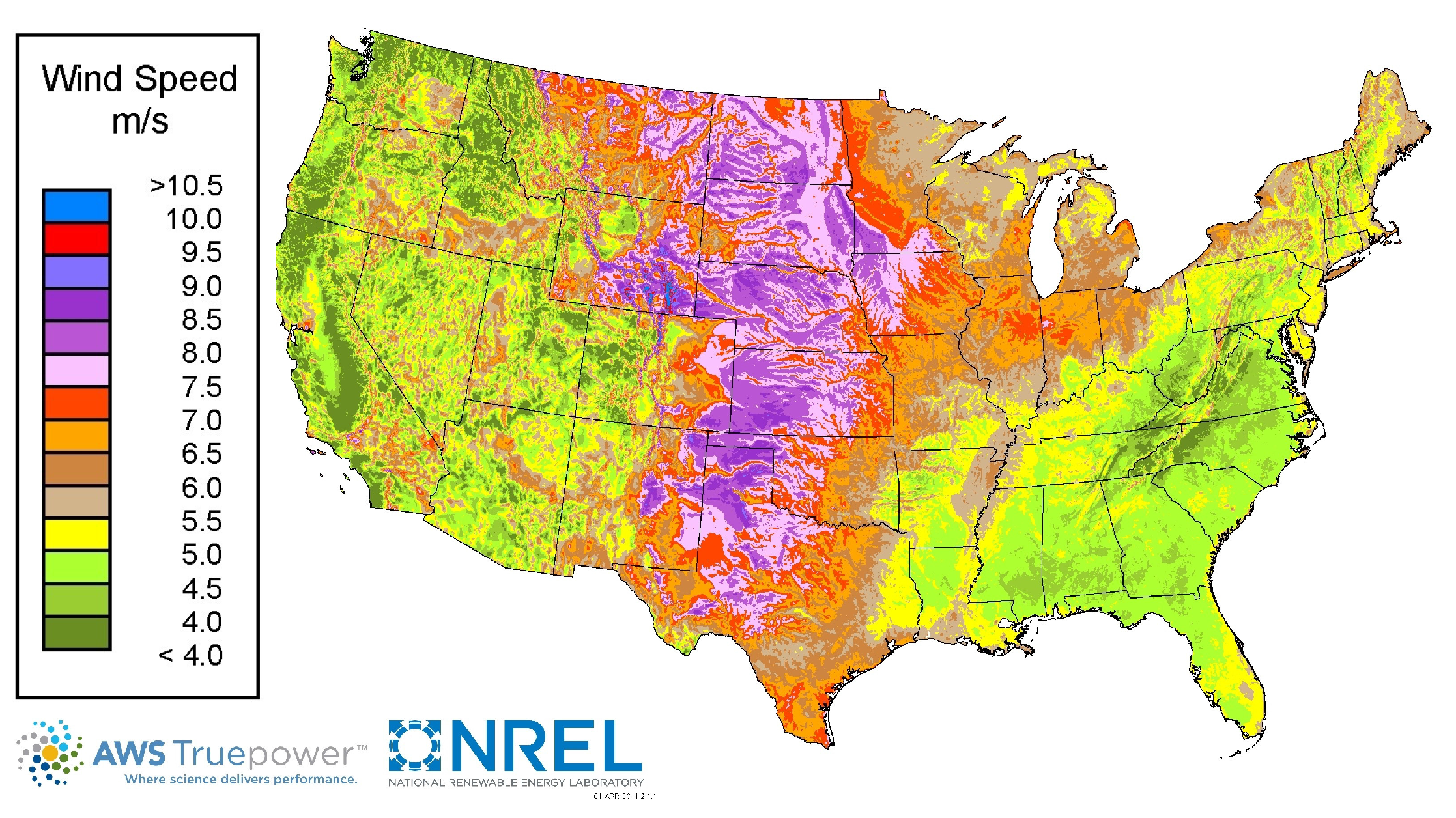
• Step 1 The geographical variation/distribution of wind regimes (in terms of AWS) in the target market is characterized; the U.S. onshore market is used as the case study.
• Step 2 The types of commercial turbines that provide the minimum COE values are determined for different wind regimes, where the minimum COE value is given by optimized arrangement of a group of such turbines.
• Step 3 The likely demand/market-suitability of the currently available (commercial) turbine feature combinations (namely, rated power, rotor diameter and hub height) is determined for the entire target market, based on the expected installation rate, geographical distribution of wind regimes (Step 1) and estimated economic potential of the best-suited turbines for different wind regimes (Step 2).
• Step 4 The tradeoffs between the cost and capacity factor offered by the best performing turbines (for different wind regimes) are also determined to explore how these tradeoffs are related to the turbine-feature combinations.

The framework developed in this paper is illustrated in Figure 1. We also develop regression models to quantify the variation of minimized COE with AWS for turbines in different rated power classes, which provides unique comparative insights into the capabilities of the commercial wind turbine systems (available in/before 2012).

The following section describes the characterization of the geographical distribution of wind regimes and the development of the comprehensive framework to determine suitable commercial turbines for different wind regimes. The optimal set of wind turbines (for different wind regimes) determined by this framework and the investigation of their economic potential with respect to AWS are presented in Section 3. Section 4 provides an exploration of the expected market suitability of commercially available turbine feature combinations to the U.S. onshore wind energy market, based on the optimization results obtained in Section 3. Section 5 explores the cost/production capacity tradeoffs offered by current commercial turbines (for different wind regimes), and also investigates the sensitivity of these tradeoffs to the features of the turbines. Section 6 presents the concluding remarks.

2. Determining Optimal Wind Turbines (under Group Operation) for Different Wind Regimes

2.1. Characterizing Wind Regimes

2.1.1. Extracting Wind Map Information

An extensive wind map for the U.S. is provided by the National Renewable Energy Laboratory’s (NREL) Geographic Information System (GIS) [21], as shown in Figure 2. This wind map shows the annual average wind speed at $80\mathrm{m}$ above ground level. The annual average wind speed (at $80\mathrm{m}$) at any location is abbreviated as AWS in the remainder of this paper. Image processing and data extraction techniques are applied to the U.S. wind map to estimate the net areas under different wind speeds in the range 3–10 m/s, corresponding to a height of 80 m above ground level. The wind map data used in this research do not include the states of Alaska and Hawaii. The annual AWS data corresponds to a resolution of 1/3 degrees of latitude by 1/4 degrees of longitude. It can be seen from Figure 2 that the onshore wind resource in the U.S. varies approximately between average wind speeds of 4.0 m/s and 9.0 m/s at a height of 80 m above ground level. This variation spans a range of wind resource strengths from Class 1–Class 5 [20].

MATLAB image processing tools (The MathWorks Inc.: Natick, MA, United States) are used to extract average wind speed (AWS) information from the wind map (Figure 2) at a resolution of $1700\times 2200$ pixels (noise attributed to text labels in the map are filtered out). Each AWS regime thus spans over 0.5 m/s, where the range under consideration goes from 3.5 m/s–10.0 m/s; thus, the area under different AWS values is assigned to $13\times 0.5\mathrm{m}/\mathrm{s}$ bins. Wind speeds below 3.5 m/s represent marginal wind resources and are not feasible for wind energy development. Hence, locations with AWS below 3.5 m/s are excluded from the target market for wind turbine installation. All onshore land area that experiences AWS above 3.5 m/s is treated as prospective wind farm sites and is therefore a part of the turbine market. In reality, a substantial portion of this land area is neither suitable nor available for wind farm development, owing to factors, such as: (i) forests/protected vegetation; (ii) human establishments; (iii) industry; (iv) environmental restrictions; (v) complex topography; (vi) agricultural land; and (vii) distance from major gridlines. The consideration of these factors is not within the scope of this paper. It is thus important to note that the explorations performed in this paper are subject to the approximations and assumptions generally made in the creation of wind maps; and when dedicated wind data become available at the region-wide scale, they should serve as the preferred source of wind resource information in such explorations (instead of wind maps).

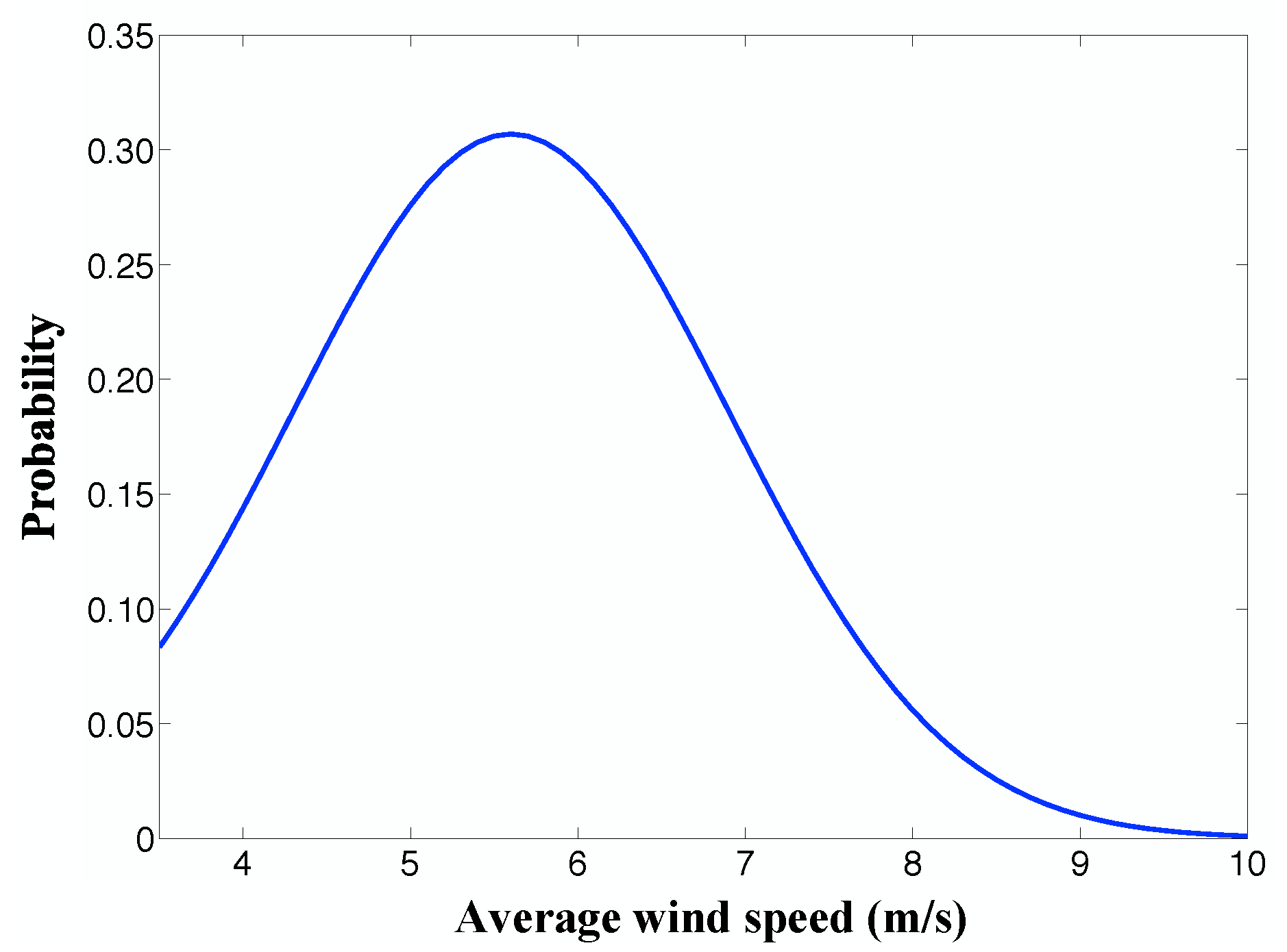
2.1.2. Distribution of Wind Regimes in the Target Market

A normal distribution is used to represent the occurrence frequency of AWS over the contiguous mainland U.S. (as illustrated in Figure 3). Wind farm optimization is performed for different AWS values to identify the best performing turbines for those wind regimes. The probability of the AWS value in the concerned target market in this case provides a measure of the likely market demand of the corresponding optimally-selected turbine. It is observed that the distribution of the average onshore wind speed (in the U.S.) has a mean of 5.6 m/s and a standard deviation of 1.3 m/s.

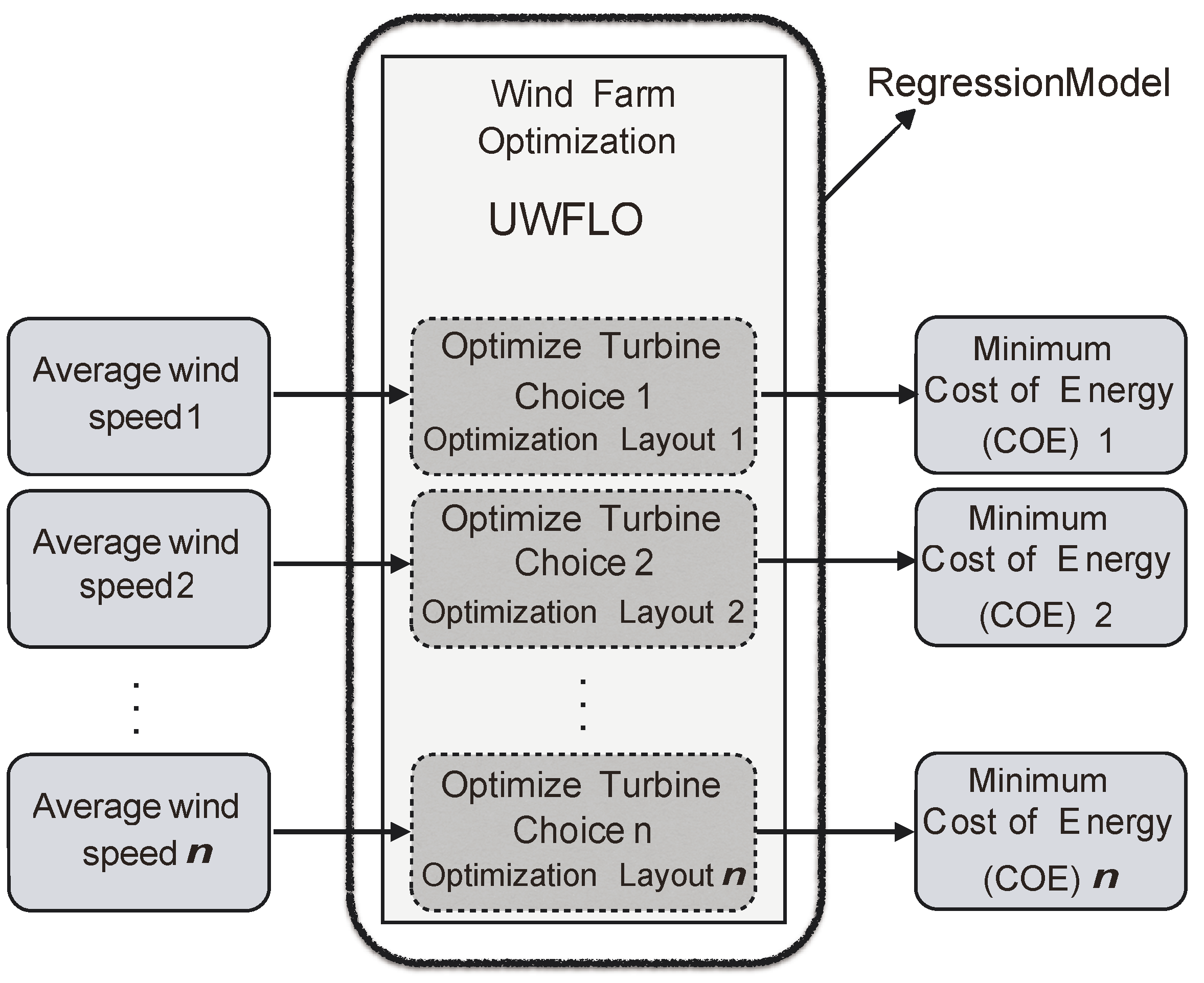
2.2. Approach to Determine Optimal Turbine Choices

The choice of operating conditions-compatible turbines (in this paper) is based on which turbine type(s) leads to the lowest cost of energy (COE) for the wind farm. It is important to note that, in this paper, we focus on the suitability of turbines across various wind regimes primarily in terms of their ”energy production capacity (when operating in a group)” and cost. The former factor is unique to exploring different wind regimes with a varying footprint in a region. Other criteria, such as structural compatibility (which would require atmospheric boundary layer turbulence code), noise impact and local/regional market share of different manufactures, are not taken into consideration in this paper. The COE of a farm depends both on the cost of the turbines (installed) and on the performance of the turbines as members of a group of optimal micro-sited turbines. The COE is minimized for a given nameplate capacity by simultaneously optimizing the selection and the placement of the turbines in the farm. To this end, we use the unrestricted wind farm layout optimization (UWFLO) framework developed by Chowdhury et al. [8,9].

In the UWFLO power generation model [8], the incoming wind is assumed to follow a log profile [26]. The growth of the wake downwind of a turbine, also accounting for wake merging scenarios, is determined using the wake growth model proposed by [27]. The corresponding energy deficit downwind of a turbine is determined using the velocity deficit model developed by [28], which is widely used in wind farm power generation estimation [14,15,29,30,31]. The UWFLO power generation model also accounts for the possibility of a turbine being ‘partially’ in the wake of another turbine located upwind. The net power generated by the wind farm, for a given incoming wind condition, is evaluated by the sum of the powers generated by the individual turbines. The wind farm power generation model developed in UWFLO has been successfully validated by [9] against published experimental data [32].

The energy production over a defined time period is determined by integrating (numerically) the power generation function over the distribution of wind speed and direction (estimated for that time period). The wind turbine design cost and scaling (WTDCS) model, reported by [33], is adopted to estimate the cost of the farm attributable to the turbines installed. The farm dimensions and the allowed minimum distance between any two turbines are treated as constraints during optimization. An advanced mixed-discrete particle swarm optimization algorithm [34] is applied to perform the optimization.

In order to determine optimal turbine choices for different wind regimes, a set of 25 sample AWS values is generated using Sobol’s quasirandom sequence generator [35] in the range of interest determined in the previous Section (i.e., $3.5–10\mathrm{m}/\mathrm{s}$). Sobol sequences are often exploited as a sampling strategy due to their reasonably beneficial space-filling (or uniform experimental design) properties [36]. Sobol sequences use a base of two to form successively finer uniform partitions of the unit interval and then reorder the coordinates in each dimension. Here, each sample AWS value represents a wind regime, for which we intend to determine the best performing turbines (in terms of COE) through wind farm layout optimization. However, an important factor to consider in this context is: The power generated by a turbine is proportional to the third degree of the approaching wind speed. Since wind speeds vary significantly over time, using a uniform incoming wind speed equivalent to the sample AWS can significantly bias this exploration. To mitigate such bias, we instead use the one-parameter Rayleigh distribution to account for the wind speed variations; this distribution is estimated by using the sample AWS as its mean. The Rayleigh distribution is a special case of the more descriptive Weibull distribution (with the Weibull shape parameter equal to two) and can be expressed as: $f\left(x\right)=\frac{x}{{\sigma }^2}exp\left(\frac{-x^2}{2{\sigma }^2}\right)$. The mean of the Rayleigh distribution is given by $\mu =\sigma \sqrt{\pi /2}$. Therefore, for a location with an AWS of s m/s (which can be practically assumed to be the mean of the wind distribution), the parameter σ of the Rayleigh distribution can be determined by:

$$\sigma =s\sqrt{{\displaystyle \frac{2}{\pi }}}$$

(1)

For illustration purposes, a set of 10 sample AWS are generated, which is representative of 10 different wind regimes. The Rayleigh distributions corresponding to the 10 sample AWS are shown in Figure 4. If dedicated data is available, more flexible wind uncertainty models, e.g., Weibull and kernel density estimation-based distributions, can be leveraged to model the wind speed variations and make more accurate estimates of wind energy production, with the rest of the framework (presented in this paper) remaining the same. It is important to note that for sites where the most descriptive Weibull distribution of wind speed has a shape parameter that is significantly larger than two, the use of the Rayleigh distribution could introduce noticeable inaccuracies. However, when solely depending on average wind speed values from a wind map (which is the practical scenario when considering an entire region), the Rayleigh distribution provides a unique solution towards accounting for wind uncertainties in the process of estimating the average energy production. Moreover, if dedicated wind data is available at a region-wide scale, it would also be possible to determine the coupled distribution of wind speed and direction and the turbulence intensities, which will allow more comprehensive estimation of energy production capacity and the likely consideration of structural compatibility factors. It is important to note in this context that the UWFLO method leveraged in this paper (to identify optimal turbine choices under group operation) can readily consider various aspects of wind characteristics (including turbulence intensity) through the flexibility of using different wake models [37].

The nameplate capacity and the land dimensions of the farm are fixed with a small tolerance for nameplate capacity, as multiples of all available rated power values may not exactly match the equality constraint associated with the specified nameplate capacity. A circular wind farm shape is assumed to avoid any directional bias that could be introduced if a rectangular farm shape (with fixed aspect ratio) is assumed [38]. The area of the circular farm, $A_{farm}$, is expressed as a function of the allowed land-area per MW installed, as given by:

$$A_{farm}=t\times max\left(D^2/P_r\right)\times P_{NC}$$

(2)

where $P_{NC}$ represents the specified (fixed) nameplate capacity of the farm, and t is an integer. The parameters D and $P_r$ respectively represent the generic rotor diameter and the rated power of commercial turbines. Based on land use data from 172 individual wind energy projects in the U.S., NREL reported average area usage as $34.5\pm 22.4$ hectares/MW [39]. With a specified $t=21$ in this paper, the above formula thus allows a meager 11.7 hectares/MW of land area for the wind farms to be optimized; such a stringent land footprint specification promotes turbines and layout plans that can have minimum impact on the farm surroundings (an important factor to consider in wind farm development). The following two subsections describe how we quantify the performance of each turbine and the cost attributable to each turbine.

2.3. Turbine Characterization Model

Every turbine is defined in terms of the five primary features that influence its power generation performance: (i) rated power; (ii) rated speed; (iii) rotor-diameter; (iv) hub-height; and (v) power characteristics. The rotor-diameter and the hub-height of a turbine determines which part of (and what extent of) the wind shear profile experienced by the turbine. They also regulate the characteristics of the wake produced by the turbine. Hence, for an array of turbines, the rotor-diameter and the hub-height play important roles in regulating the overall mutual shading effects and the subsequent energy availability within the farm. The specification of these two features is readily available (in online brochures) for most commercial wind turbines.

The rated power, the rated speed and the power characteristics can be used to determine the power generated by the turbine for any given incoming wind. These three properties are implicit to the power curve, if available. However, information regarding the “power vs. wind speed” variation is not readily available for many of the 131 commercial turbines allowed for selection in this study; generally, the rated power and the rated speed are specified by the manufacturer. Hence, a generalized power curve ($P_n$) is developed using the manufacturer reported data for a 1.5 MW wind turbine [40]. To this end, a fifth degree polynomial is fitted to the graph data. The power generated (P) and the incoming wind speed (U) are normalized with respect to the rated power ($P_r$) and rated speed ($U_{rated}$), respectively. Here, the incoming wind speed is given by the rotor-averaged wind speed estimated from the wind information at a given height (which is 80 m for the NREL wind map), assuming a log profile of wind shear [41].

Using this generalized power curve ($P_n$), the rated power, the cut-in, cut-out and rated speed reported by different manufactures, the power curve of other commercial turbines can be approximated as:

$${\displaystyle \frac{P}{P_r}}=\left\{\begin{array}{c}{P}_n{\displaystyle \frac{U-U_{in}}{U_r-U_{in}}},\mathrm{if}{U}_{in}\le U<U_r\hfill \\ 1,\mathrm{if}{U}_r\le U<U_{out}\hfill \\ 0,\mathrm{if}{U}_{out}\le U\mathrm{or}U<U_{in}\hfill \end{array}\right.$$

(3)

where $P_n$ represent the polynomial fit for the normalized power curve. This generalized power characteristics estimation strategy has been used for ready implementation purposes; if the power response data are available for a particular wind turbine, a unique power curve specific to that turbine should be ideally determined and used.

2.4. Wind Turbine Cost Model

Since the mid-1990s, wind turbine configurations have become more standardized. As a result, the development of a generic model to estimate the cost of wind turbine components became possible. Around this time as well, the Department of Energy (DOE) launched the Wind Partnership for Advanced Component Technology (WindPACT) projects. The aim of these projects was to investigate ways to achieve cost reductions in wind turbine production. The extension of the WindPACT projects came about when [33,42] prepared a wind turbine design cost and scaling (WTDCS) model for the then-modern wind turbine configurations, based on 2002 U.S. dollars. According to the WTDCS model, the cost of a farm attributed to one turbine, ${\mathrm{C}}_{\mathrm{FT}}$, can be expressed as:

$$C_{\mathrm{FT}}=C_{\mathrm{MF}}+C_{\mathrm{BS}}+C_{\mathrm{LR}}+C_{\mathrm{OM}}$$

(4)

where $C_{\mathrm{MF}}$, $C_{\mathrm{BS}}$, $C_{\mathrm{LR}}$ and $C_{\mathrm{OM}}$ represent the total manufacturing cost, the balance-of-station cost, the levelized replacement cost (LRC) and the operation and maintenance (O&M) cost (all costs are in U.S. Dollars), respectively.

In the WTDCS model, the annual operation and maintenance cost is represented as a linear function of the annual energy production (AEP), i.e., $C_{\mathrm{OM}}=0.007\times AEP$, which does not adequately account for the dependency of the O&M cost on the turbine features and the site location (geography and wind pattern). Instead, this function places turbines with a higher energy production capacity (for a given resource) at a disadvantage, which is not entirely realistic. At the same time, for onshore turbines, the O&M cost is a small fraction of the total cost of the farm. Therefore, we do not include the O&M cost in the wind farm cost model used in this paper.

The manufacturing cost, $C_{\mathrm{MF}}$, is an aggregate of the turbine component costs. The component costs are represented in the WTDCS model as functions of the following important features of the turbine: rotor diameter, hub height and machine rating (rated power). In this paper, we provide the mathematical expressions for the cost of the major components of a turbine, which include the blades, gearbox, generator, variable-speed electronics and tower. Detailed formulations of the component costs can be found in [33]. The blade cost is given by the sum of the blade material cost and the labor cost, both of which are defined in terms of the rotor diameter. The blade cost, $C_{\mathrm{BL}}$, is expressed as:

$$C_{\mathrm{BL}}=\left((0.05\times D^3-21,051.00)+(0.4843\times D^{2.5025})\right)/(1-0.28)$$

(5)

where D denotes the rotor diameter of the turbine (in meters).

The estimation of the costs of gearboxes and generators is generally challenging owing to the various configurations available. The WTDCS model considered four different configurations that include (i) the three-stage planetary/helical gearbox with high-speed generator; (ii) the single-stage drive with medium-speed generator; (iii) the multi-path drive with multiple generators; and (iv) the direct drive with no gearbox. Till recently, a majority of the available wind turbines were equipped with the three-stage gearbox-based drive-train with the high-speed generator. However, in the past decade, direct-drive turbines have started to become popular as well. The gearbox cost and the generator cost ($C_{\mathrm{GB}}$ and $C_{\mathrm{GN}}$) for the three-stage drive and the generator cost of the direct-drive ($C_{DGN}$) are given below:

$$\begin{array}{c}\mathrm{Three}-\mathrm{stage}\mathrm{gear}:C_{\mathrm{GB}}=16.45\times P_r^{1.249};C_{\mathrm{GN}}=65.00\times P_r\hfill \\ \mathrm{Direct}-\mathrm{drive}:C_{DGN}=219.33\times P_r\hfill \end{array}$$

(6)

where $P_r$ denotes the rated power (in kilowatts). Assuming that the turbine has a power convertor, the total cost of the variable-speed electronics ($C_{\mathrm{VE}}$) is expressed as:

$$C_{\mathrm{VE}}=79.00\times P_r$$

(7)

The cost of the tower can be represented as a function of its weight (in kilograms), which in turn is expressed as a function of the hub height and the swept area. The weight ($M_{\mathrm{TW}}$) and the cost ($C_{\mathrm{TW}}$) of a tower made of advanced materials are given by:

$$\begin{array}{c}{M}_{\mathrm{TW}}=0.2694\times A_S\times H+1779.00\hfill \\ C_{\mathrm{TW}}=1.50\times M_{\mathrm{TW}}\hfill \end{array}$$

(8)

In Equation (8), H is the hub height of the turbine (in meters), and $A_S$ is swept area (in square meters) given by $A_S=\pi D^2/4$.

The balance-of-station cost ($C_{\mathrm{BS}}$) primarily includes the costs of roads and civil work ($C_{\mathrm{RC}}$) and that of electrical connections ($C_{\mathrm{EC}}$); these costs [42,43] are given by:

$$\begin{array}{c}{C}_{\mathrm{RC}}=P_r\times (0.00000217\times P_r^2-0.0145\times P_r+69.54)\hfill \\ C_{\mathrm{EC}}=P_r\times \left(0.00000349\times P_r^2-0.0221\times P_r+109.70\right)\hfill \end{array}$$

(9)

The levelized replacement cost in terms of U.S. dollars ($C_{\mathrm{LR}}$), which includes the costs of long-term replacements and the overhaul of the major turbine components, is given by:

$$C_{\mathrm{LR}}=10.70\times P_r$$

(10)

Further details of the assumptions and the cost formulation of other wind turbine components can be found in [33]. The WTDCS cost model used in this study particularly considers and is applicable for those turbine configurations that have been (over the years) popular in the commercial industry, which includes the three-bladed, upwind, pitch-controlled, variable-speed wind turbine and its variants. The general configuration of three-bladed wind turbines has changed marginally since 2006. Hence, the cost model developed by Fingersh et al. [33] is practically applicable to compare costs of commercial turbines available in 2012 in the market.

2.5. Optimization of Farm Layout and Turbine Type Selection

For each sample average wind speed (AWS) value in the range 3.5–10.0 m/s, wind farm optimization is performed to minimize the cost of energy (COE). The COE in terms of U.S. dollars for a candidate farm is given by:

$$COE={\displaystyle \frac{N\times C_{\mathrm{FT}}}{E_{farm}}}$$

(11)

where N is the number of turbines in the farm, $C_{FT}$ is the cost of the farm attributed to one turbine and $E_{farm}$ is the annual energy production of the wind farm. The annual energy production (AEP), $E_{farm}$, is estimated by numerically integrating the UWFLO power generation model over the Rayleigh distribution of wind speed associated with the concerned AWS value. The Monte Carlo integration technique is employed [8] using a set of 20 random wind speed values in the range 3.0–25.0 m/s. Other assumptions for the generic wind farm are summarized in

Table 1. Specified properties of the generic wind farm site.

Property	Value
Nameplate capacity	25.0 MW
Radius of the circular farm	964.0 m
Average terrain roughness	0.1 m (grassland)
Density of air	1.2 kg/m${}^3$

.

The objective function in the minimization problem is the COE of the wind farm, and the design variables are the locations of each turbine ($X_j$,$Y_j$) and the type of turbine (T) to be used, i.e., a total of $2N+1$ design variables for an N-turbine wind farm. The optimization problem is therefore defined as:

$$\begin{array}{c}\mathrm{Min}f\left(V\right)=COE\hfill \\ \mathrm{subject}\mathrm{to}\hfill \\ g_1\left(V\right)\le 0\hfill \\ g_2\left(V\right)\le 0\hfill \\ V=\left\{X_1,X_2,......,X_N,Y_1,Y_2,......,Y_N,T\right\}\hfill \\ 0\le X_j\le R_{farm}\forall j=\left\{1,2,\dots ,N\right\}\hfill \\ 0\le Y_j\le R_{farm}\forall j=\left\{1,2,\dots ,N\right\}\hfill \\ T\in \left\{1,2,\dots ,T^{max}\right\}\hfill \end{array}$$

(12)

where the parameter $T^{max}$ represents the number of turbine-types allowed for selection. The parameter $R_{farm}$ represents the radius of the farm, given by $R_{farm}=\sqrt{A_{farm}/\pi }$, where $A_{farm}$ is given by Equation (2). The constraint $g_1$ ensures a minimum required clearance between adjacent turbines, and the constraint $g_2$ ensures that the turbines are located within the fixed circular farm boundaries [44].

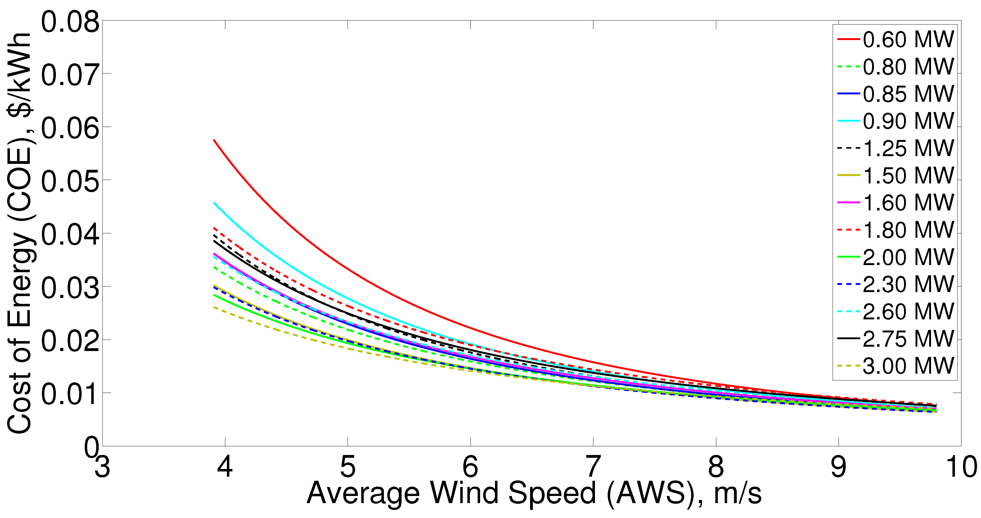
3. Pool of Optimal Turbine Choices for Differing Wind Regimes

For a given installed capacity of the wind farm, the number of turbines in the farm is automatically determined by the choice of the turbine rated power. In the UWFLO method, simultaneous optimization of turbine selection and placement involves $2N+1$ design variables, i.e., $2N$ turbine coordinates and one turbine type indicator. Hence, differing choices of rated powers yield candidate farm designs with differing numbers of design variables. Such candidate designs with different variable space dimensions cannot be typically optimized together. Therefore, for each sample AWS, optimization is performed separately to identify the optimal turbine (for that AWS) from each rated power class. In this paper, we test 131 commercial turbines, belonging to 13 different rated power classes available from seven major global turbine manufacturers (in 2012).

Table 2. Major commercial turbine choices in the U.S. onshore market.

Rated-Power Class (MW)	Number of Available Choices	Number Installed in the Farm
0.60	3	42
0.80	7	31
0.85	13	29
0.90	3	28
1.25	6	20
1.50	16	17
1.60	5	16
1.80	10	14
2.00	36	13
2.30	14	11
2.60	3	10
2.75	4	9
3.00	11	8

lists the rated power classes and the numbers of turbine variants in each class. It is important to note that the effective installed capacity of the farm is fixed at $25\pm 1$ MW, to allow a realistic number of turbines (to be installed) for each rated-power class.

For a set of n random AWS values and the allowed 13 different turbine rated power classes (Table 2), wind farm optimization is required to be performed $13n$ times, which can become computationally expensive. Through numerical experiments, we found that a sample size of $n=25$ provides an acceptable representation of the geographical distribution of AWS at a reasonable computational expense for the $13n$ optimization runs. For each sample AWS, the results of the 13 optimizations corresponding to the 13 different turbine rated-power classes are compared to determine the best turbine choice across all classes. Figure 5 shows what rated-power turbines perform the best (under an optimized layout operation), i.e., provide the lowest COE, for different AWS values.

It can be observed from Figure 5 that the 3 MW turbines performed the best for lower values of AWS (<6.5 m/s), while the 2.3 MW turbines performed the best for higher wind speeds (>6.5 m/s). Only for the AWS value of 7.15 m/s, a 1.5 MW turbine performed the best. Higher rated-power turbines (generally with larger swept areas) can extract more energy from the wind, thereby delivering higher capacity factors; hence, they are suitable for sites with low average wind speeds. For higher average wind speeds, the likely greater cost of these higher rated-power turbines (compared to low rated-power turbines) generally offsets the benefits of their greater energy extraction capability. In that case, lower rated-power turbines, which are generally less expensive and provide reasonable capacity factors, become more suitable for sites with higher average wind speeds. Interestingly, it is also found that all of the 25 best performing turbines are of the direct-drive type. This observation shows that direct-drive turbines are capable of delivering competitive COE compared to turbines with the conventional three-stage gear drive-train; which conforms with the ongoing industry shift from the conventional gear-based drive-train to the direct-drive system [45,46,47,48]. However, further investigation is necessary, through turbine scale analysis, to fully compare and contrast these two turbine drivetrains, which is not within the scope of this paper.

In this paper, with the consideration of COE as the performance objective, cost and energy production capacity are treated as the underlying measures of performance. In practice, there exist other measures of the quality/behavior of a wind turbine, which also play important roles in deciding suitable turbine choices for a given site. Examples of such measures include: (i) structural performance of the turbine components with respect to the dynamic loading experienced under a given set of wind conditions; (ii) the relative ease of transportation and installation w.r.t. the given site; (iii) the maintainability of turbine components; and (iv) the availability of turbine models and their operational and performance histories. Hence, more flexible illustrations of turbine performance with regard to AWS are provided here. Figure 6 shows how the minimum COE accomplished by the best performing turbines from each rated-power class (obtained through wind farm optimization) varies with the AWS. Figure 7 shows how the capacity factor accomplished by these best performing turbines from each rated-power class varies with the AWS. Figure 8 shows the costs of the optimized wind farm configurations, based on the costs of the corresponding best performing turbines. The cost measures are expressed in terms of the hourly cost per kW installed ($/kWh). The hourly cost per kW installed is obtained by dividing the total farm cost by “$365\times 24\times t_{years}$”, where the lifetime of the wind farm, $t_{years}$, is assumed to be 20 years; the “hourly cost per kW installed” is illustrated in Figure 8 to serve as a readily-perceivable unit-measure of turbine costs (independent of turbine ratings), which is referenced later in this section to aid the discussion of the findings regarding optimal turbine choices across different wind regimes.

Expectedly, the minimized COE decreases with increasing AWS (Figure 6). It is also observed that beyond 7.0 m/s, the decrease in COE is marginal. Overall, lower COE values are accomplished by the (best performing) higher-rated power turbines. However, there are exceptions to this trend. Figure 6 shows that contrary to the general trend, the commercially available 0.8 MW turbines performed better (particularly for low AWS) than turbines in the following higher rated-power classes: 0.85 MW, 0.90 MW, 1.25 MW, 1.60 MW, 1.80 MW, 2.60 MW and 2.75 MW. Similarly, the commercially available 1.50 MW turbines performed better (particularly for low AWS) than turbines in higher rated-power classes of 1.60 MW, 1.80 MW, 2.60 MW and 2.75 MW. With the exception of the 0.90 MW turbine class, all of these other “higher-rated yet dominated” turbine classes did not have direct-drive variants available (among the ones used in this paper), unlike the 0.80 MW and 1.50 MW rated-power classes. However, due to the lack of availability of dedicated power curve data for each of the 131 turbines, the above observation does not necessarily provide clear evidence as to the comparative performance of turbines with direct drive and conventional gear box transmission systems.

Interestingly, for higher average wind speeds (i.e., AWS > 8.0 m/s), the deviation in “minimum COE obtained” across turbines of different rate-power classes is less than 25%. Smaller (lower rated-power) turbines are thus relatively more competitive at this end of the wind regime spectrum, especially when we also consider the following factor: larger turbines are generally associated with greater cost and logistic challenges with regard to their transportation, installation and component replacement (and attractive wind farm sites are often found in remote locations that are poorly connected). Some of these challenges may not be adequately captured in most existing wind farm cost models, including the WTDCS cost model adopted here. It is also important to note that the cost of the best performing turbines itself does not follow any particular trend with respect to rated power (owing to the impact of component-size variation across similarly rated turbines), as readily evident from Figure 8. Based on the WTDCS cost model [33], it is found that among the comprehensive set of wind turbines considered here (from the 2012 or earlier market), the 0.9 MW turbines are the least expensive and the 1.8 MW turbines are the most expensive.

Although the power generated by a stand-alone turbine is proportional to the cubic degree of the approaching wind speed (assuming uniform flow), the capacity factor of the optimized farm is observed to follow more of a linear variation with AWS (Figure 7). This observation can be primarily attributed to the use of a distribution of wind speeds (instead of a constant AWS) and the effect of wake losses within the farm. Based on this capacity factor variation trend, the minimized COE is expected to vary as an inverse polynomial function of the AWS; this hypothesis conforms with the observed trends in Figure 6. We therefore performed inverse polynomial regression (response surface) to formulate a uniquely helpful analytical expression representing the minimum COE as a function of AWS, corresponding to each rated-power class as illustrated in Figure 9. The generic expression can be represented as:

$$COE=c_1{s}^{c_2}$$

(13)

where $c_1$ and $c_2$ are unknown coefficients, such that $c_1$ > 0 and $c_2$ < 0; s represents the AWS. The regression curves, corresponding to the 13 turbine rated-power classes, are shown in Figure 10. The coefficient values and the accuracy measures of the regression curves are provided in

Table 3. Details of the polynomial regression curves: representing the variation of minimized COE with AWS (for each turbine class).

Rated-Power Class (MW)	$c_1$	$c_2$	R${}^2$ value	RMS Error
0.60	1.190	−2.222	0.9720	0.0027
0.80	0.363	−1.746	0.9691	0.0015
0.85	0.447	−1.845	0.9741	0.0015
0.90	0.725	−2.028	0.9895	0.0012
1.25	0.526	−1.897	0.9797	0.0015
1.50	0.299	−1.684	0.9791	0.0011
1.60	0.414	−1.789	0.9722	0.0016
1.80	0.474	−1.796	0.9837	0.0013
2.00	0.239	−1.563	0.9792	0.0010
2.30	0.293	−1.676	0.9850	0.0009
2.60	0.369	−1.716	0.9753	0.0014
2.75	0.430	−1.769	0.9783	0.0015
3.00	0.184	−1.433	0.9784	0.0009

. It is readily evident from the R${}^2$ values (>0.96) and the root-mean-squared (RMS) error values (<0.003) given in Table 3 that the regression fits are accurate. We observe that the minimized COE, accomplished by the best performing turbines of each rated-power class, is generally proportional to −1.4 down to −2.8 power of the AWS (i.e., an inverse linear-quadratic function of AWS). It is important to note that this observation is conditional on the land area allowed for turbine installation (specified in this paper), and such COE estimates are generally sensitive to nameplate capacity and land area/MW installed.

In Figure 11a,b, the rotor diameter and the hub height (tower height) are respectively shown for the best performing turbines in each rated-power class for different AWS. It can be seen that different turbine variants were often chosen from each rated-power class for different AWS values; this observation is evident from the cost illustration as well (Figure 8). Some of the higher rated-power turbines, those with greater rotor diameters and higher hub heights (and which are also generally more expensive), were in most cases preferred for low average wind speeds. For the majority of the other turbine classes, no such trend was readily evident. It was observed in Figure 6 that even though direct-drive variants were available in the 0.90 MW rated-power class and were the least expensive (Figure 8), in terms of COE, these turbines were noticeably outperformed by the best performing 0.80 MW turbines. This seemingly counterintuitive phenomenon can be attributed to the substantially smaller rotor diameters and the lower tower heights of the 0.90 MW turbines (Figure 11a,b), which limits the amount of power these turbines can extract from the wind. This behavior is also evident when we observe that among all rated-power classes, the lowest capacity factors are yielded by the best performing 0.90 MW turbines (Figure 7). Further investigation of the market-wide suitability of various turbine feature combinations is provided in the following section.

4. Market Suitability of Turbines

4.1. Development of a Market Suitability Metric for Wind Turbines

In this section, we explore the suitability (likely demand) of currently available turbines for the U.S. market. The overall market suitability of available turbine features is represented in terms of the selection likelihood of the available turbine feature combinations (of rated power, rotor diameter and hub height). The selection likelihood of turbine feature combinations is defined as a function of:

• How often different feature combinations were selected during the $13\mathrm{n}$ wind farm optimizations, across the different wind regimes (from Section 3);
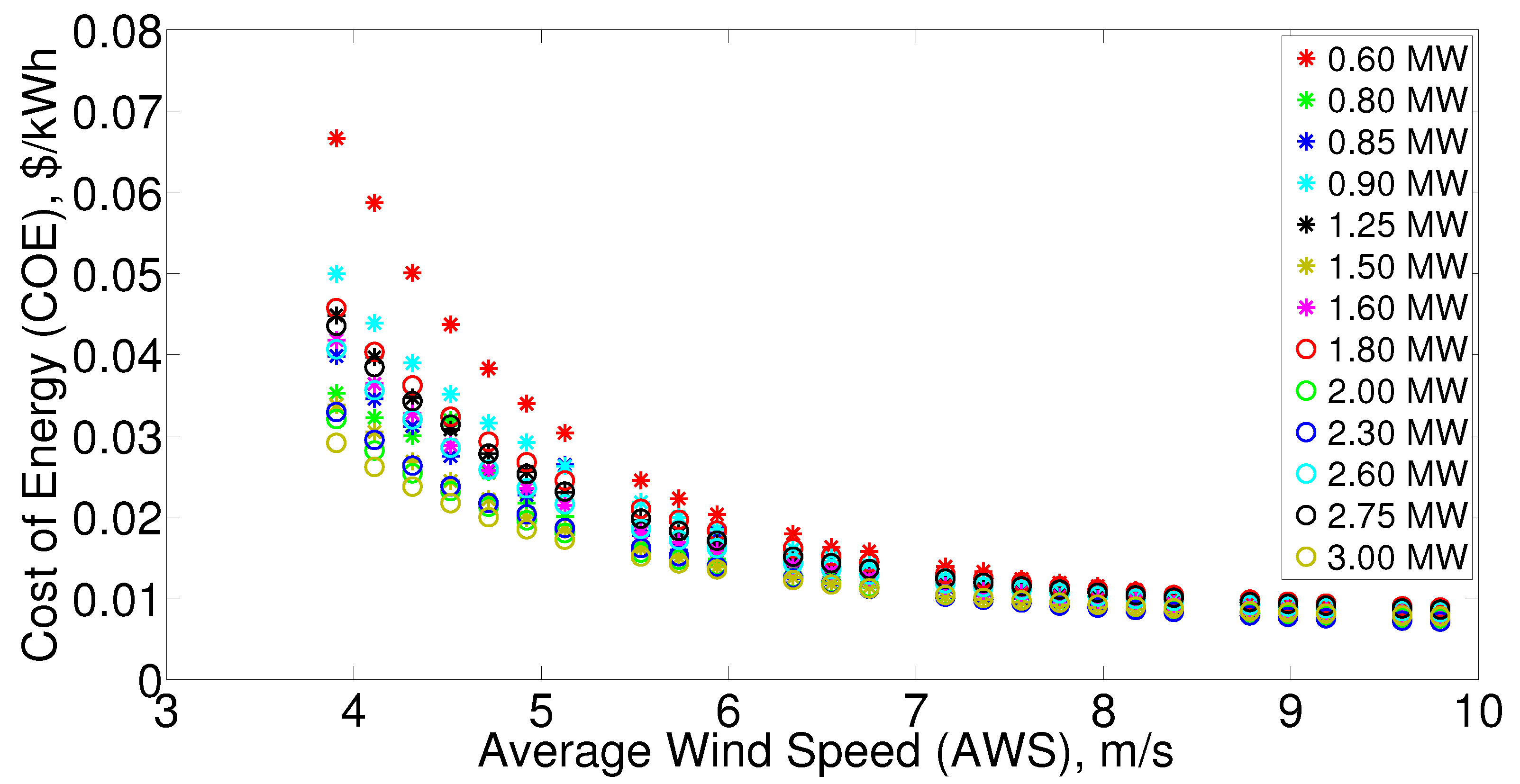
• What level of performance (in terms of COE) was offered by the best performing turbines (from each rated-power class); and
• The probability of occurrence of each of the n sample average wind speeds (for which wind farm optimization was performed) over the U.S. onshore market; determined in Section 2.1.

The performance-based expected suitability (PES), S, of a turbine is defined over the entire range of wind resources (i.e., all wind regimes) as:

$$\begin{array}{c}{S}_i={\displaystyle \sum _{j=1}^n}{\delta }_i^j{\displaystyle \frac{CO{E}_{min}^j}{CO{E}_i^j}}\hfill \\ where\hfill \\ {\delta }_i^j=\left\{\begin{array}{c}1,\mathrm{if}\mathrm{the}i-\mathrm{th}\mathrm{turbine}\mathrm{was}\mathrm{selected}\mathrm{for}\mathrm{the}j-\mathrm{th}\mathrm{sample}\mathrm{AWS}\hfill \\ 0,\mathrm{if}\mathrm{the}i-\mathrm{th}\mathrm{turbine}\mathrm{was}\mathrm{not}\mathrm{selected}\mathrm{for}\mathrm{the}j-\mathrm{th}\mathrm{sample}\mathrm{AWS}\hfill \end{array}\right.\hfill \end{array}$$

(14)

where the subscript i refers to the $i-\mathrm{th}$ commercial turbine among the 131 allowed types (i.e., $i=1,2,\dots ,131$). The parameter $CO{E}_{min}^j$ represents the lowest value of the minimized COE accomplished (among all rated-power classes) for the $j-\mathrm{th}$ sample AWS; the parameter $CO{E}_i^j$ represents the minimized COE accomplished for the $j-\mathrm{th}$ sample AWS, by the rated-power class to which the $i-\mathrm{th}$ commercial turbine belongs. It is important to note that the suitability of turbines in each rated-power class is scaled using the relative COE values, which lends helpful flexibility to the measure of suitability.

In order to provide measures of the likely market success (market suitability/demand), the suitability indices ($S_i$) are scaled by the corresponding probability of the sample AWS in the concerned region: the U.S. onshore market. Therefore, the performance-based expected market suitability (PEMS) is estimated as:

$${\overline{S}}_i=P_M\sum _{j=1}^n{\delta }_i^j{\displaystyle \frac{CO{E}_{min}^j}{CO{E}_i^j}}{p}_s^j$$

(15)

where $p_s^j$ represents the probability of occurrence of the $j-\mathrm{th}$ sample AWS in the target market region. The parameter $P_M$ represents the total wind power potential in GW of the target market region. According to Equation (15), the PEMS of a commercial turbine (${\overline{S}}_i$) is conveyed in terms of the total gigawatts of likely installation of that turbine in the target market. As estimated by NREL [49], a total wind power potential value of 10,459 GW at an 80 m height for the contiguous United States (which excludes Hawaii and Alaska) is used in this paper. Only windy land area with a gross capacity factor of >30% at an 80 m height is considered, based on the NREL wind map [21] used in this paper (Figure 2). NREL’s estimate of the overall wind power potential excludes protected lands (e.g., national parks and wilderness) and incompatible lands (e.g., urban, airports, wetland and water features). For this investigation, we have assumed that the overall distribution of AWS (wind regimes) of the U.S. onshore land area in this study is similar to that of the entire contiguous United States (captured by the wind map).

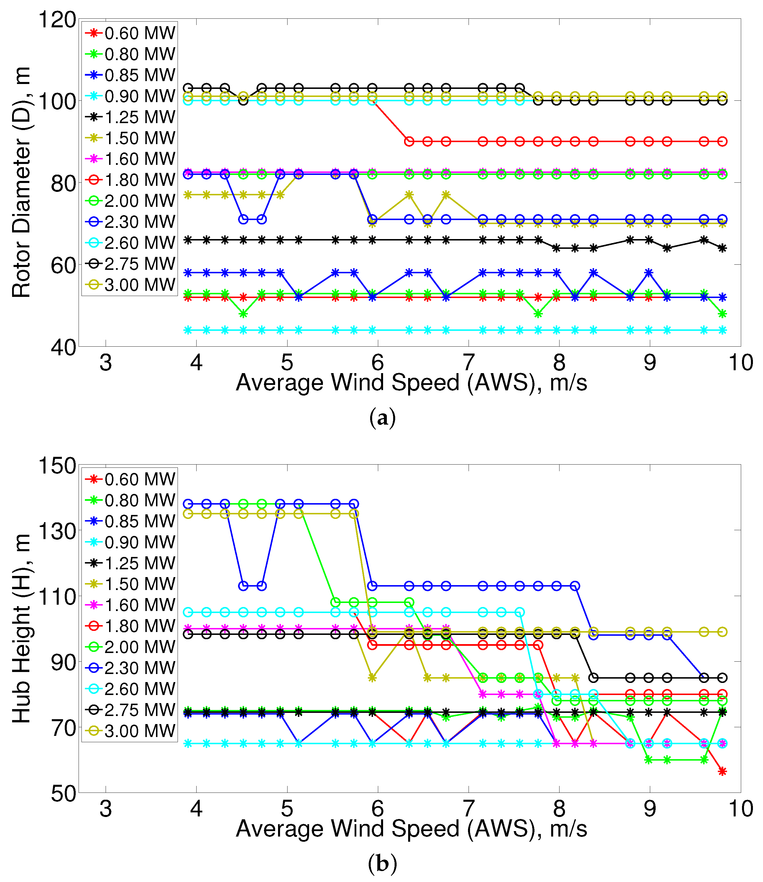
4.2. Suitability of Wind Turbine Features for the U.S. Onshore Market

The performance-based expected market suitability (PEMS) of different turbine feature combinations for the U.S. market can be readily determined from the PEMS estimates of the best performing turbines (given by Equation (15)). The PEMS of turbine feature combinations are illustrated in the form of 3D bar diagrams in Figure 12a–c, where each diagram shows two turbine features for the ease of illustration.

Figure 12a illustrates that turbines with “higher rated powers and larger rotor diameters” are the most favored among available commercial variants. Interestingly though, “higher rated-power turbines with higher hub heights” are noticeably less favored by the U.S. onshore conditions than some (not all) of the “small-medium rated power turbines (e.g., 0.8 MW and 1.5 MW) with higher hub heights” (Figure 12b). This observation might be attributed to the appreciable increase in tower costs with increasing height of the (likely large) higher rated-power turbines, resulting from material costs associated with dealing with increased structural loading. At the same time, Figure 12c shows that “turbines with larger rotor diameter and similarly sized hub heights (approximately 100 m)” are the most popular, which again indicates that relatively higher tower heights are not favored for the larger turbines. Some of the smaller turbines with rotor diameters $\le 70$ m and hub heights of approximately 75 m also display reasonable market suitability (Figure 12a–c).

It is important to note that the expected market suitability in terms of results and observations is not based on the full range of theoretically possible combinations of turbine features; it is instead based on the performance of turbines that were available from major manufacturers in or before 2012. Additionally, if the actual land area in the United States that is available for wind energy development is considered (excluding protected and incompatible land), the overall market suitability of turbine variants could be affected, as the relative frequencies of different wind regimes might change. The geographical distribution of AWS over the entire contiguous United States has a mean of 5.6 m/s at an 80 m height (Figure 2); most of the wind resource is therefore in the AWS range of 4.5–7.0 m/s at an 80 m height, i.e., wind Classes 1–4 (low to medium wind resource strengths). Hence, it is not surprising that overall, the higher rated-power turbines are preferred in the U.S. onshore market. However, for sites that are remote or that have complex terrain and that have wind classes higher than Class 4, the relatively smaller wind turbines will provide competitive and cost-effective performance. A growing market for smaller wind turbines, therefore, could continue to co-exist with the increasing demand for larger wind turbine systems. The “cost-capacity factor” tradeoffs that are provided by the best performing turbines for different wind regimes are discussed next.

5. Performance Tradeoffs Offered by Current Commercial Turbines

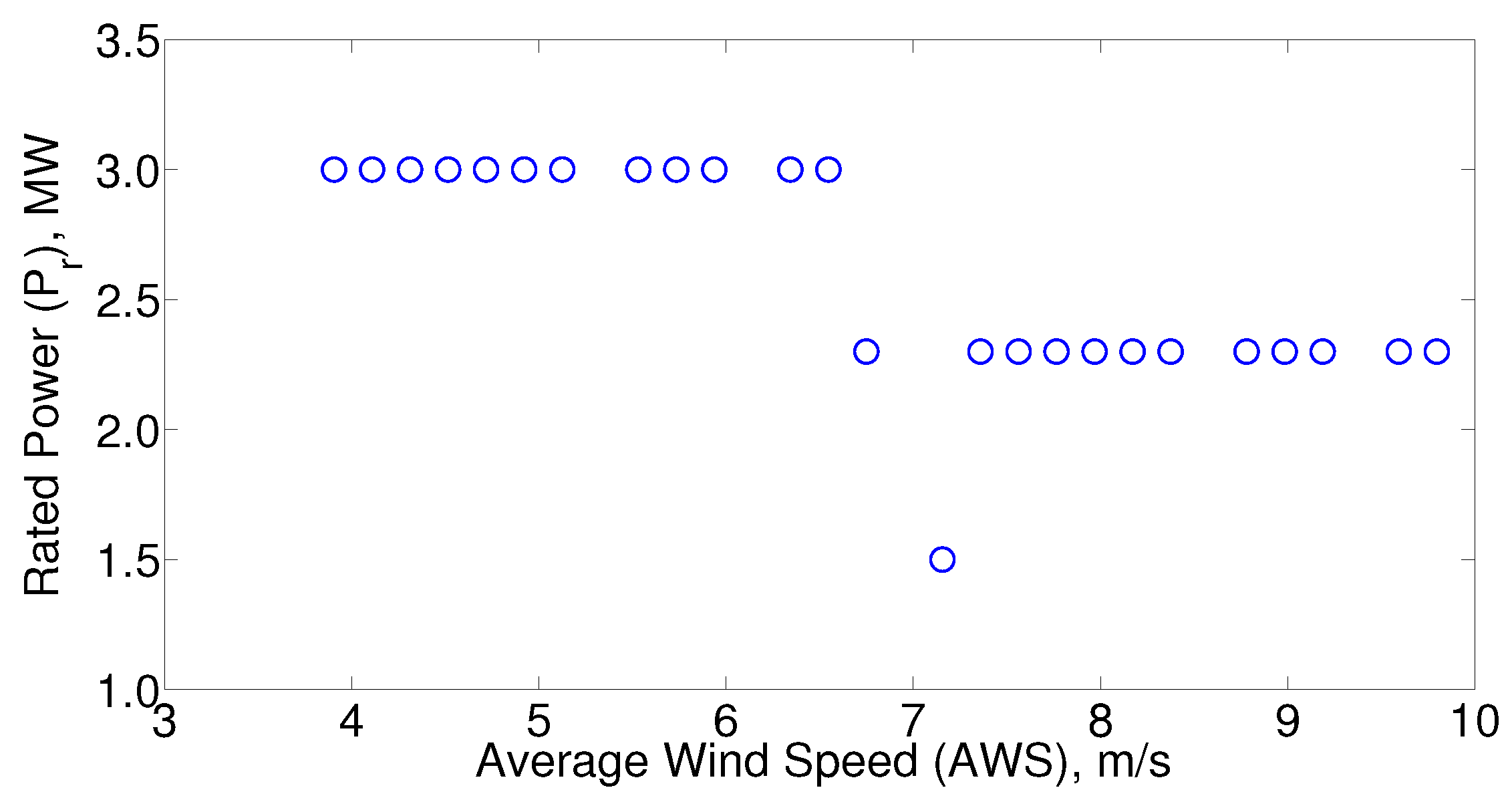
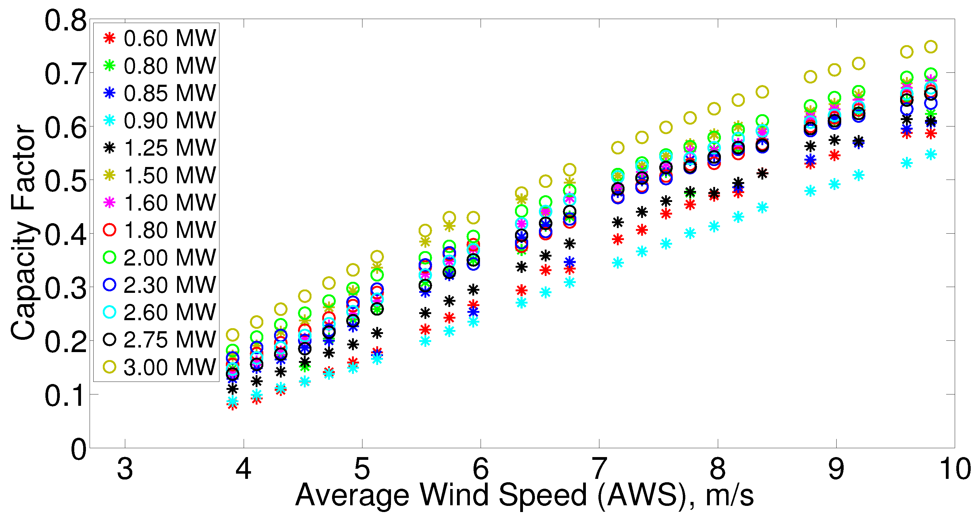
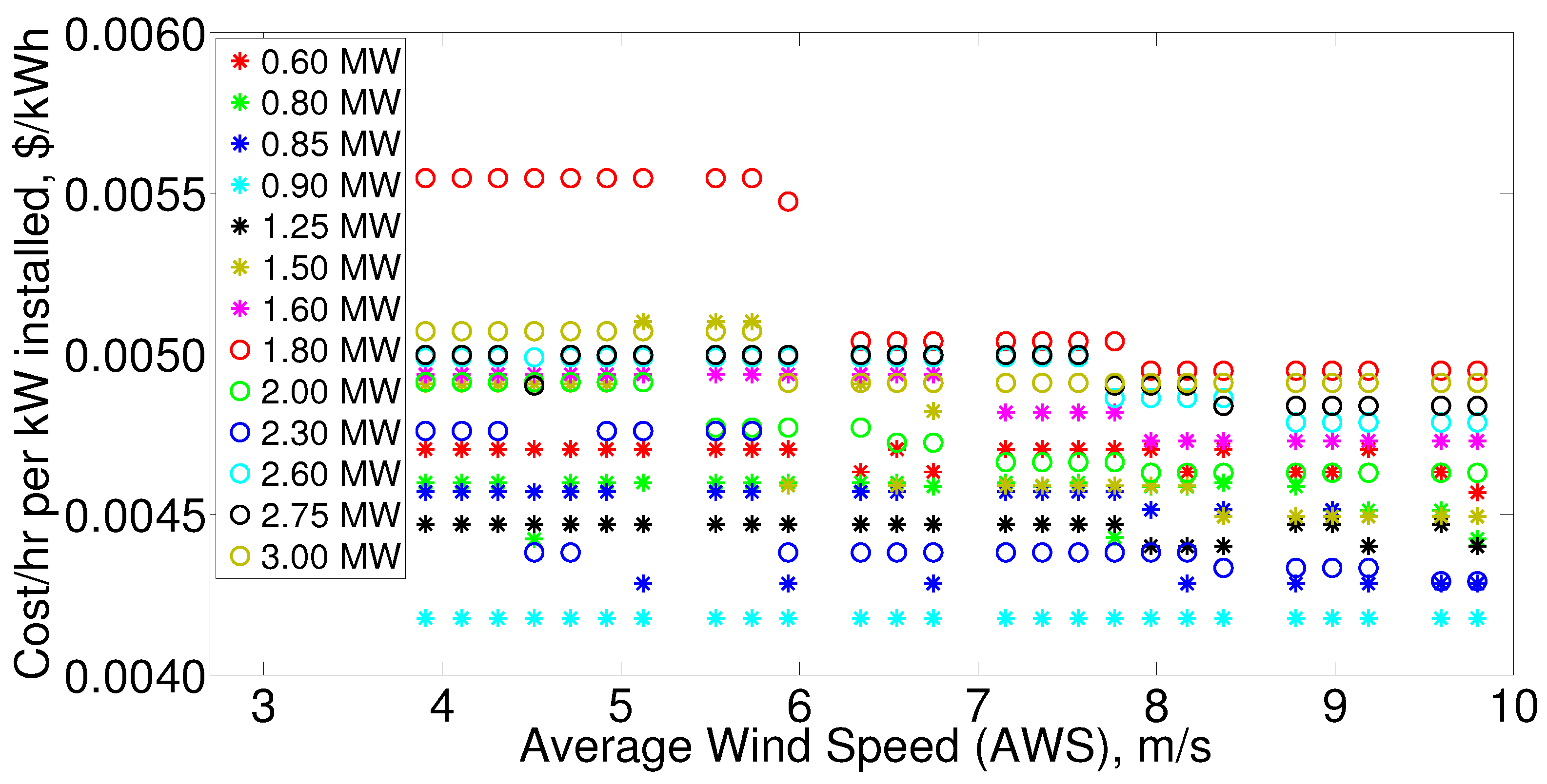
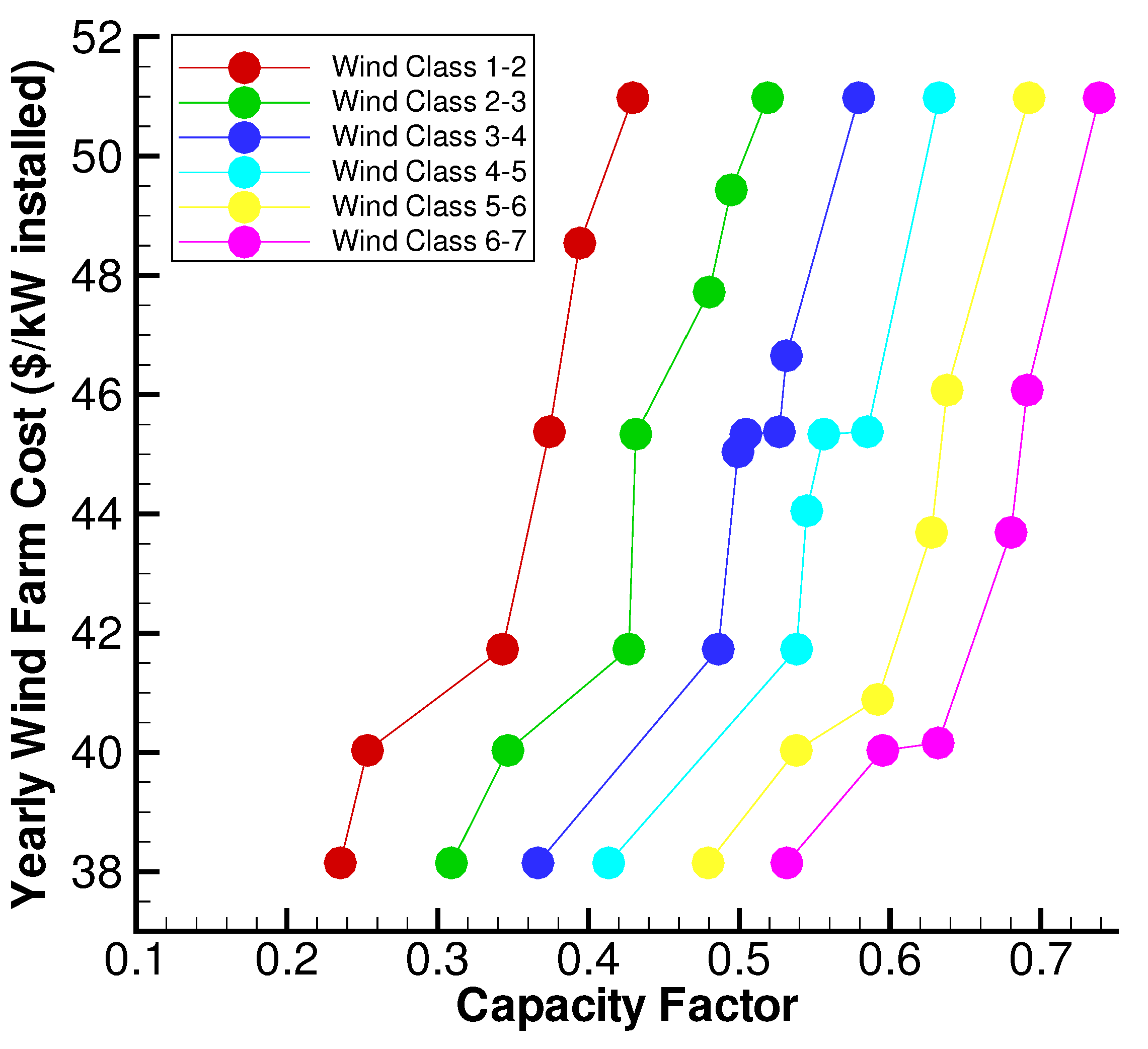
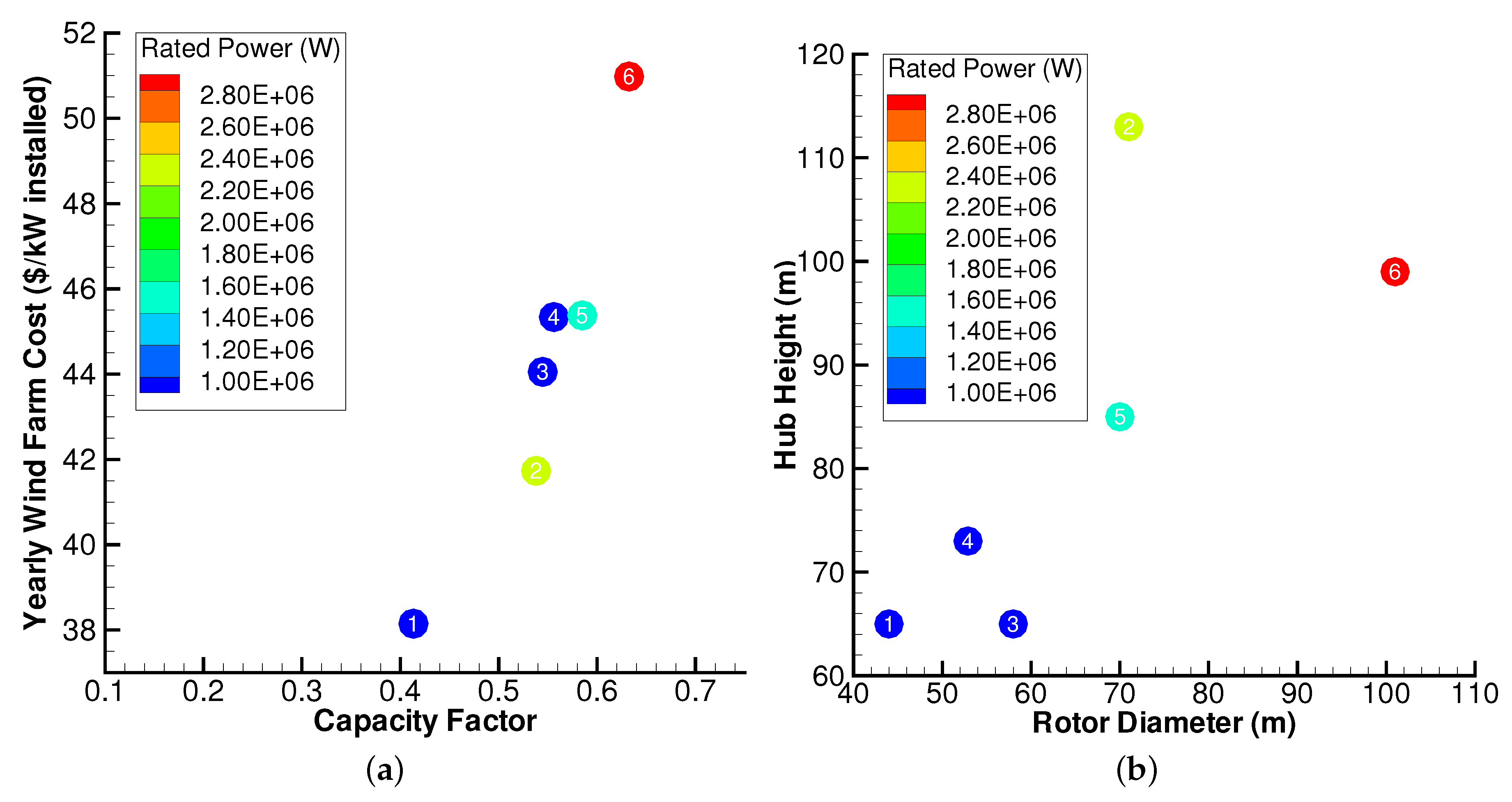
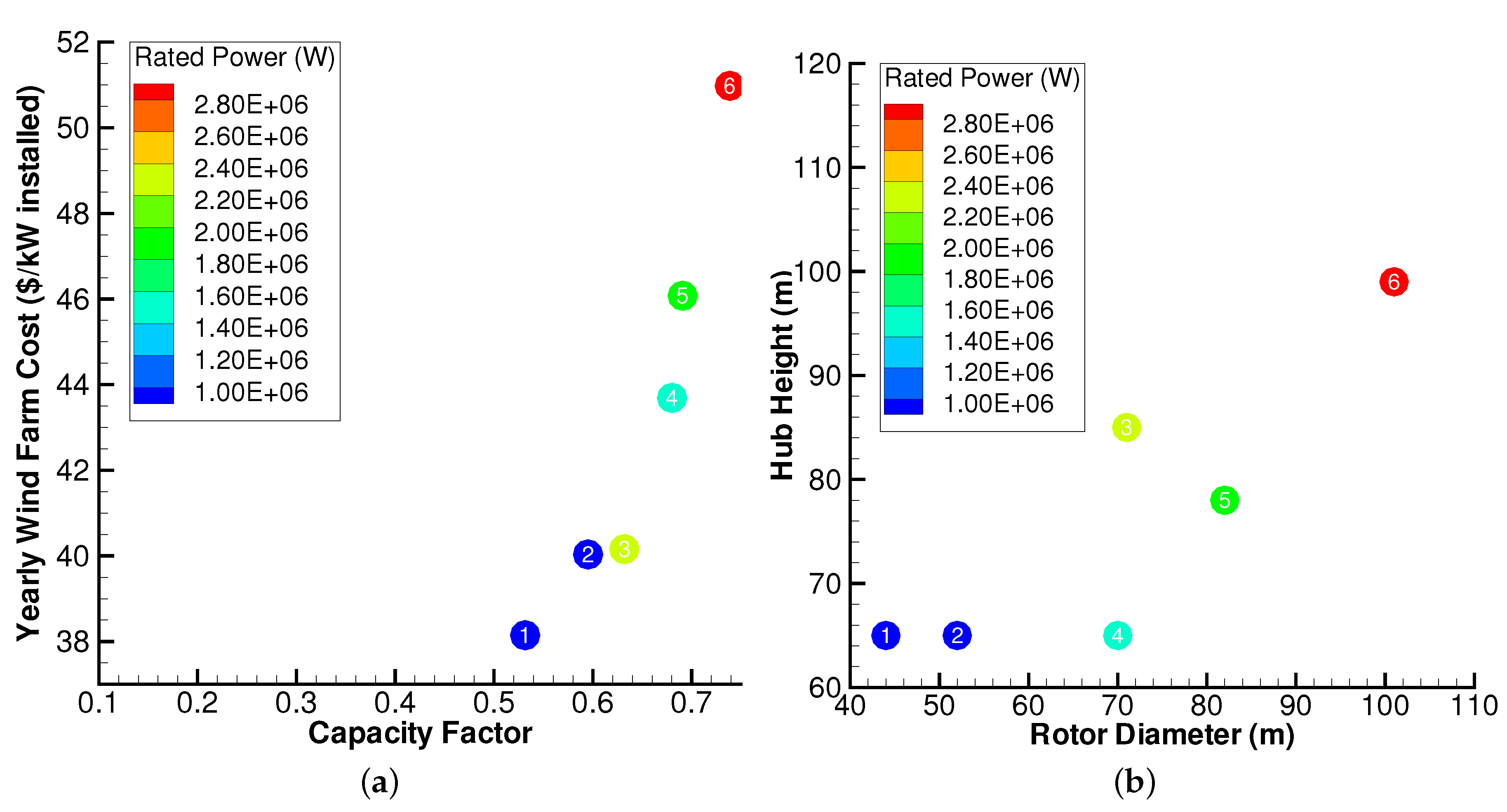
5.1. Turbine Best Tradeoffs for Different Wind Classes

The turbine suitability exploration has been performed in Section 3 in terms of COE. Although COE provides a unified understanding of the production performance and economics of wind turbines under group operation, it does not provide insights into potential tradeoffs between these two measures of turbine quality/suitability. In this section, we therefore perform an investigation of the best tradeoffs between the capacity factor and average annual cost (in $/kW installed) offered by turbines that comprise the pool of the best performing turbines (across different wind regimes) obtained in Section 3. This investigation is expected to provide further understanding of what turbine-feature combinations are expected to provide greater market value. The principle of weak dominance is used to determine the best tradeoffs in the bi-objective function space of the capacity factor and average annual cost in $/kW-installed. Considering any two generic turbines, A and B, selected from the pool of the best performing turbine obtained in Section 3, the weak dominance principle can be stated as: Turbine A is said to dominate Turbine B if and only if:

• $C{F}_A>C{F}_B\mathrm{and}Cos{t}_A\le Cos{t}_B$, or
• $C{F}_A\ge C{F}_B\mathrm{and}Cos{t}_A<Cos{t}_B$.

Here, $C{F}_A$ and $C{F}_B$ respectively represent the capacity factors of Turbines A and B under layout-optimized group operation, and $Cos{t}_A$ and $Cos{t}_B$ respectively represent the average annual cost in $/kW-installed of Turbines A and B. All CF and cost values have already been estimated in Section 3: illustrated in Figure 7 and Figure 8). The best tradeoffs are thus obtained by applying a Pareto filter to the results (i.e., estimated capacity factor and cost values) of the $13\mathrm{n}$ single objective optimizations performed in Section 3.

Among the 25 different AWS-based wind regimes studied here, for the purpose of tradeoff analysis, we choose six AWS values that closely represent the (Rayleigh distribution-based) mean wind speed values defined under the popular seven-class system [20]. For this system, NREL provides the mean wind speed and wind power density (WPD) spanning each class, considered at the heights of 10 m and 50 m. The class-defining mean wind speeds at 50 m are extrapolated using the 1/7 power law [20] to 80 m (which is the defining height of the wind map-derived AWS values used in this paper). Six AWS values (from the set of 25) are then chosen such that they closely represent the extrapolated values that separate consecutive wind classes (i.e., Classes 1–2, Classes 2–3, ... Classes 6–7) of the seven-class system. The best “cost/capacity-factor” tradeoff solutions for the six chosen AWS values are identified using a Pareto filter, as described earlier. These best tradeoffs between cost and capacity factor identified for each wind class pairs are illustrated in Figure 13.

As we move towards higher wind classes, more energy becomes available for extraction, and hence, the best tradeoff curves shift towards higher capacity factors (Figure 13). Interestingly, the best tradeoff curves corresponding to different wind classes exhibit a similar trend of variation, as seen from Figure 13. It can be observed from this figure that for an increase of $13/kW-installed in the average annual cost, the wind farm capacity factor approximately increases by 20%. Thus, from a relative perspective, this increase is more attractive at the lower end of the wind classes (where more expensive turbines thus offer greater value). Further investigation of Figure 13 shows that the initial $7/kW-installed increase in annual cost (starting from $38/kW) yields a noticeably higher increase (of 14%–15%) in the capacity factor; thereafter, the rate of capacity factor appreciation with cost reduces, where only a 5% increase is noted over the subsequent cost increment of $6/kW-installed. This observation emphasizes the potentially higher value offered by medium-priced turbines (subject to the assumptions and considerations made in this study). However, there are other factors (not explicitly considered in this study), especially those with indirect economic implications, which can also influence the relative value offered by differently-sized turbines, e.g., perceived impact of turbines of different sizes by local residents/authorities, actual impact on the surrounding environment and downtime due to natural events and planned maintenance.

The following six pairs of figures (Figure 14, Figure 15, Figure 16, Figure 17, Figure 18 and Figure 19) show the best “capacity factor-cost” tradeoffs and the features of the corresponding turbines for the six different cases, including:

• Case I: Classes 1–2 winds (Figure 14),
• Case II: Classes 2–3 winds (Figure 15),
• Case III: Classes 3–4 winds (Figure 16),
• Case IV: Classes 4–5 winds (Figure 17),
• Case V: Classes 5–6 winds (Figure 18) and
• Case VI: Classes 6–7 winds (Figure 19).

In Figure 14 to Figure 19, the “capacity factor-cost” tradeoffs in the left-side sub-figures are readily related to the corresponding “rotor diameter-hub height” combinations in the right side sub-figures by using identifying number labels. The colors of the circles represent the rated power of the corresponding turbines, as indicated in the legend included in each figure.

It is indicated by Figure 14, Figure 15, Figure 16, Figure 17, Figure 18 and Figure 19 that there exists a set of common best tradeoff turbines (i.e., similar rotor diameter-hub height combinations) across the different wind classes, particularly the 0.90 MW (44 m/65 m) and the 3.00 MW (101 m/99 m) turbines. It is also observed that the higher wind classes promote turbines with shorter towers. Interestingly, among the turbines with mid-size rotors (of approximately 70 m in diameter), some of the taller ones are observed to yield lower capacity factors while being less expensive compared to their shorter counterparts. Examples include:

• Turbines numbered 3 and 4 in Figure 14a–b,
• Turbine numbered 2 and 5 in Figure 16a–b,
• Turbine numbered 2 and 5 in Figure 17a–b,
• Turbine numbered 3 and 4 in Figure 18a–b, and
• Turbine numbered 3 and 4 in Figure 19a–b.

The above observation is counterintuitive since turbines with relatively taller tower are expected to be more expensive (due to greater tower costs) while enabling greater energy capture (thus providing greater capacity factors). This seemingly counterintuitive observation can be explained by careful investigation of the turbine power curves and of the coupled impact of rated power and hub-height of turbines (with 70 m rotors) on their cost per kw-installed.

In the five listed cases stated above, the taller turbines belong to the 2.5 MW rated power class and the shorter turbines belong to the 1.5 MW rated power class. It is found that given their rated power/speed specifications, the lower capacity factor of the taller 2.5 MW turbines can attributed to the estimated inferior power curves of these turbines (compared to the shorter 1.5 MW turbines), which compensated for the greater energy availability at greater heights from the ground.

To understand the cost comparison in these cases, using the WTDCS model, we provide a contour plot (Figure 20) of the average annual cost (in $/kw-installed) as a function of the rated power and hub height of turbines with 70 m rotors diameters. From Figure 20, it is readily evident that the cost per kw-installed is relatively more sensitive to the rated power that to the hub height, in the given ranges. Hence, for the five listed cases stated above, the higher rated 2.5 MW turbines turn out to be less expensive per kw-installed than their 1.5 MW counterparts.

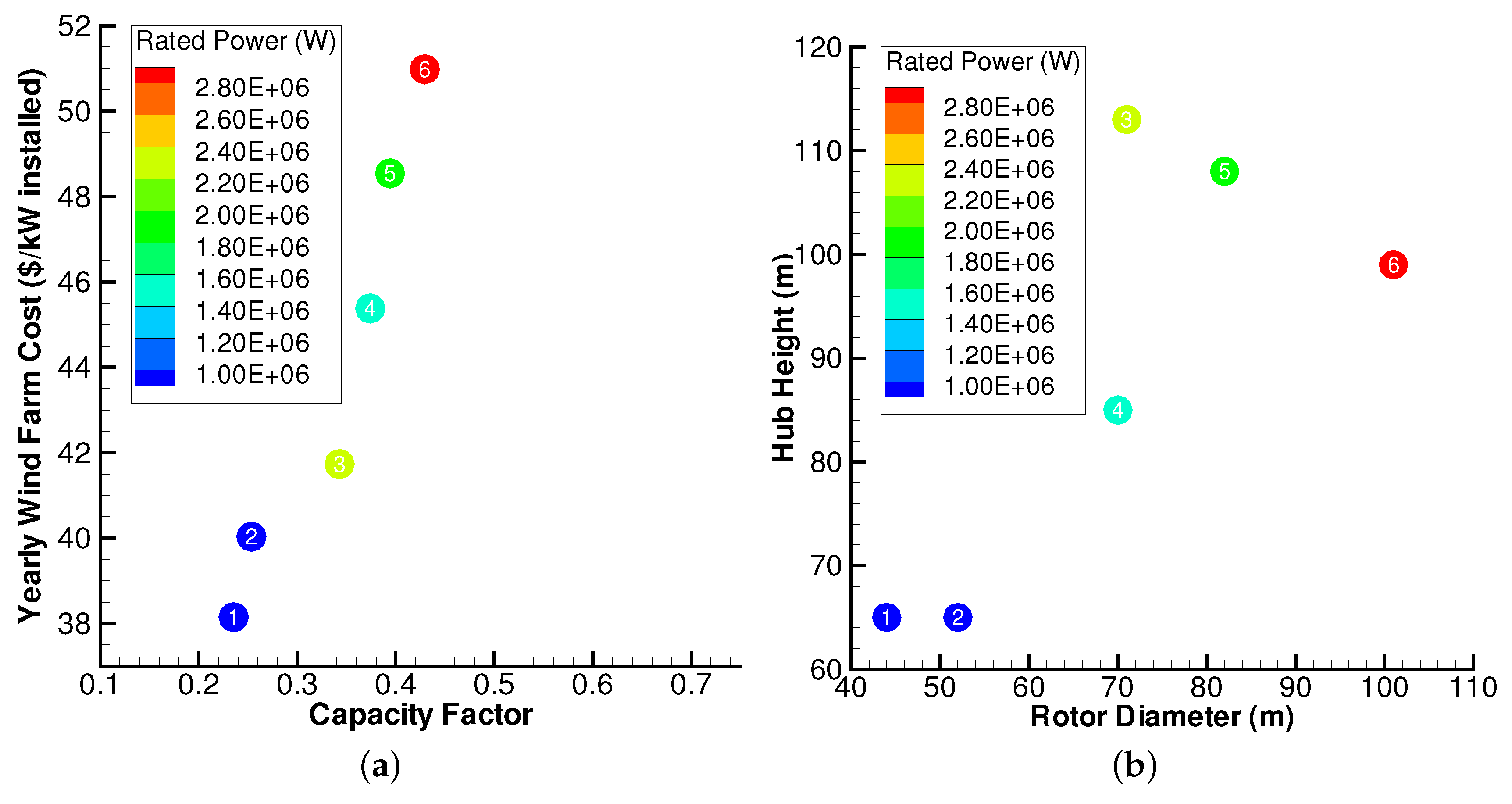
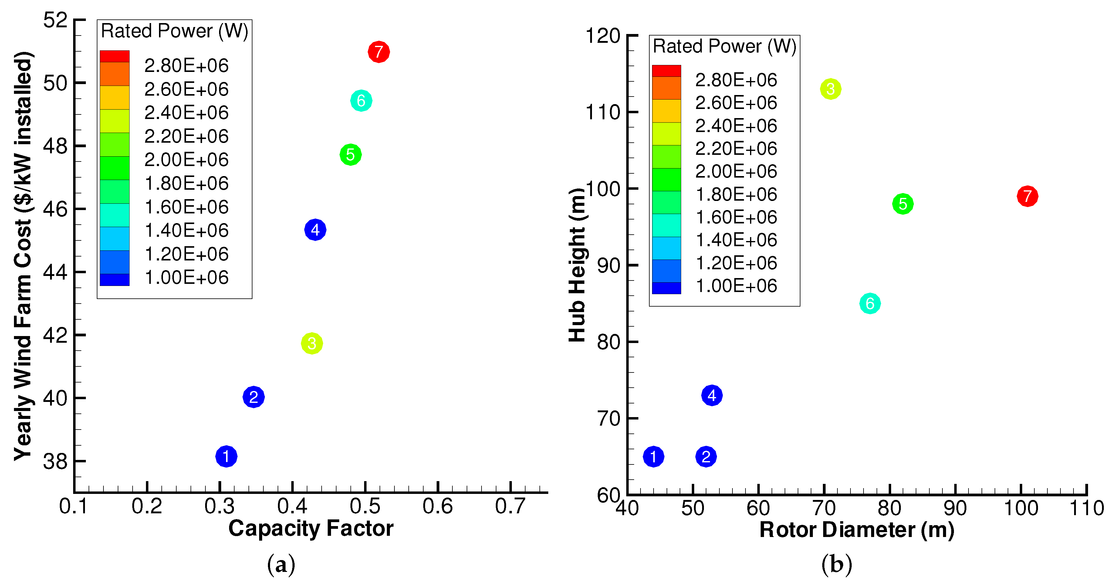
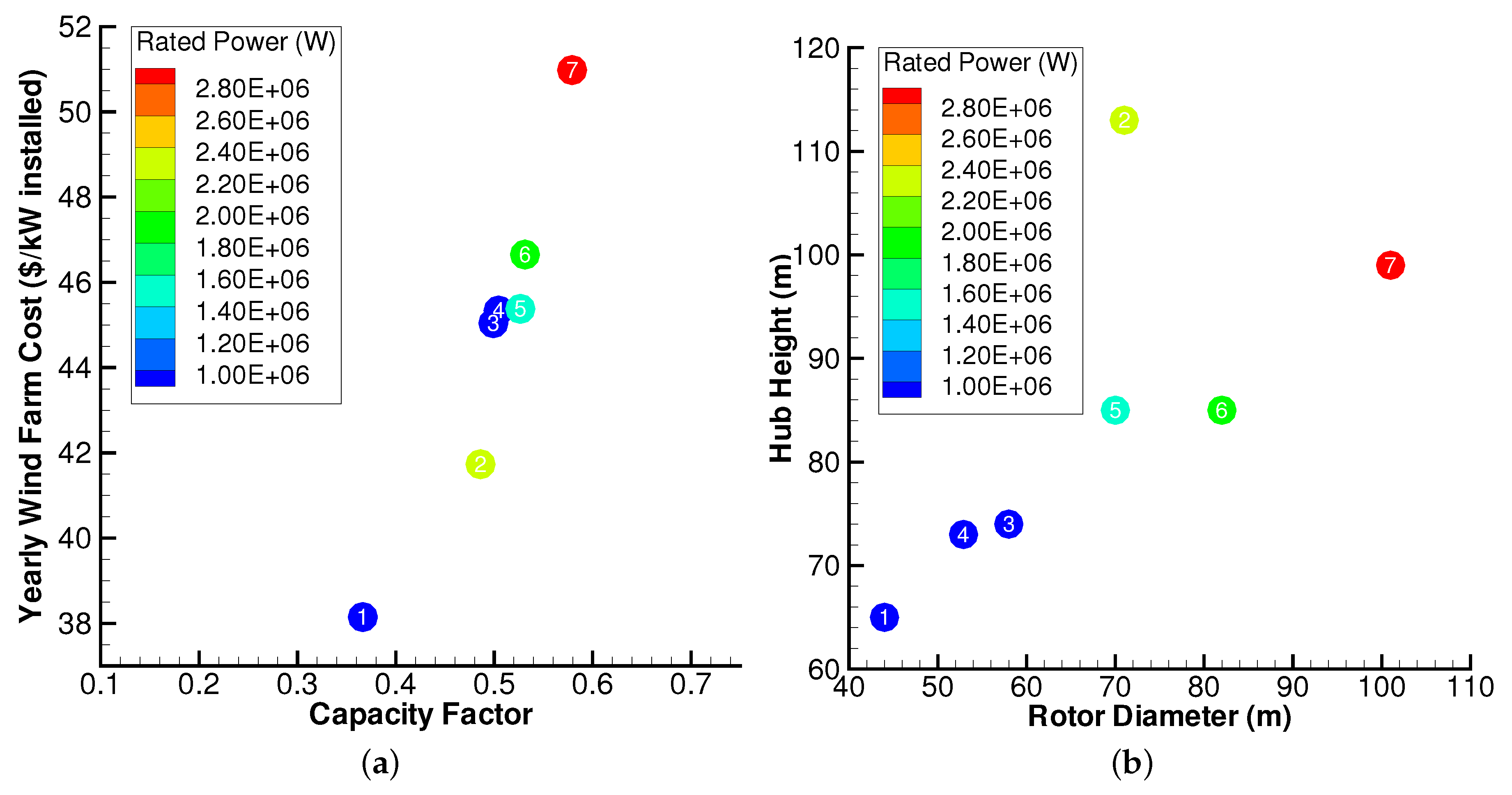
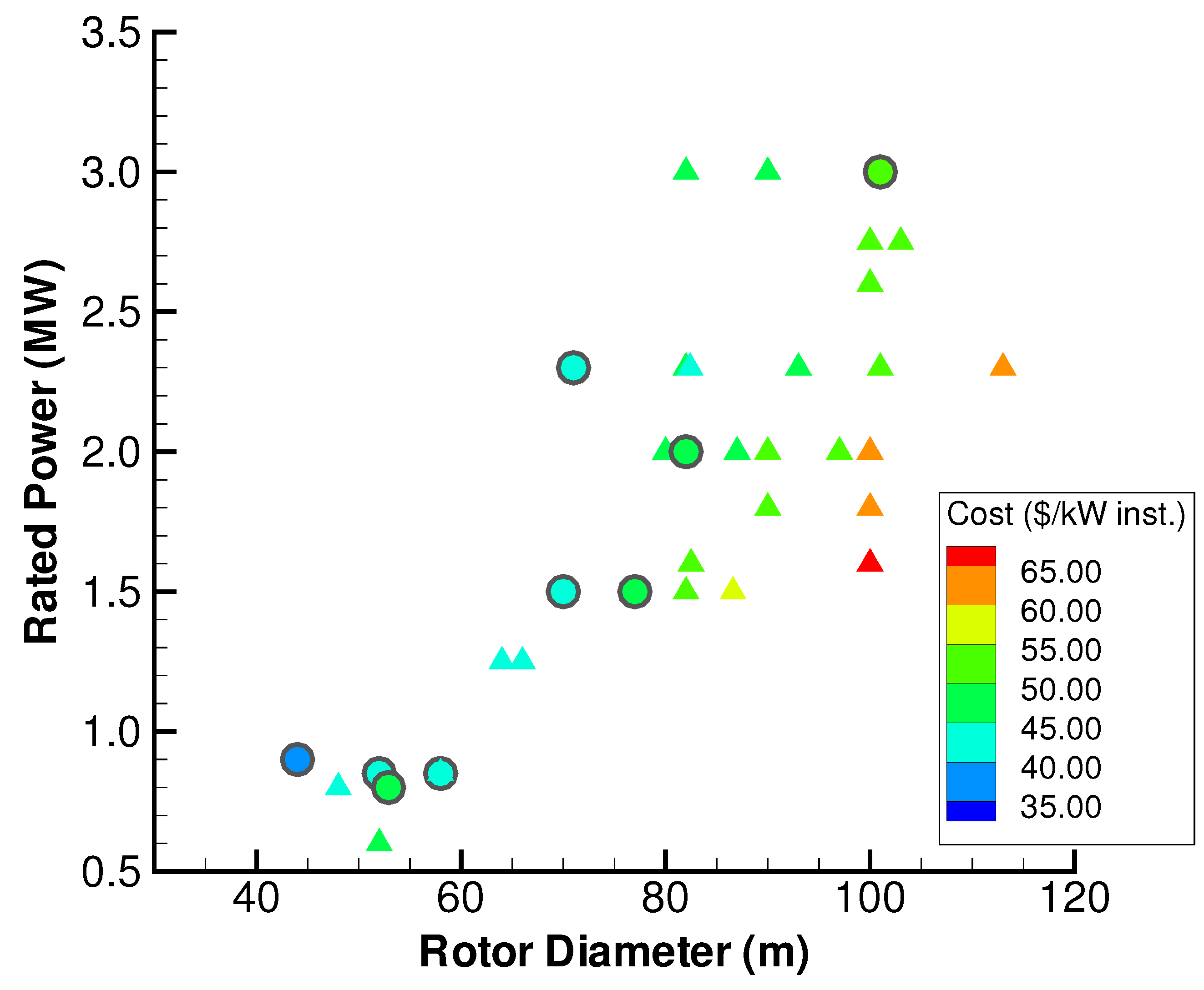
5.2. Comparing the Features of the Best Tradeoff Turbines to those of all Turbines Considered

The feature combinations of the best tradeoff turbines (identified in Section 5.1) are now compared to those of other dominated turbines in the candidate pool of 131 turbines considered in this paper. This comparison is performed to investigate why certain ranges of turbine features provide better tradeoffs in terms on cost per kW-installed and energy production capacity (under layout-optimized group operation).

Figure 21 shows the rated power and rotor diameter combinations of both the best tradeoff turbines (considering all wind classes) and the other dominated turbines; the former is represented by circles and the latter by triangles in Figure 21, both symbols being colored in terms of the cost per kW-installed.

It is observed from Figure 21 that the best tradeoff turbines span almost the entire range of rated powers and rotor diameters (excluding the 113 m rotor). For turbines in the 1.5–2.5 MW range, larger rotors are observed to be less preferable (Figure 21), which can be likely attributed to the higher costs (per kW installed) associated with larger rotors. We also observe (from Figure 21) that while the best tradeoff turbines (circles) cost less that $50/kW-installed per year, the 1.5–2.5 MW turbines (with relatively larger rotors) cost approximately $50–65/kW-installed. The greater wind shadowing effects of larger rotors in the group operation of turbines often offsets the gain in energy extraction at the individual turbine scale (associated with a larger swept area).

Figure 22 shows the rotor diameter and hub height combinations of both the best tradeoff turbines (considering all wind classes) and the other dominated turbines; the former is again represented by circles and latter by triangles in Figure 22, both symbols being colored in terms of the cost per kW-installed. In this figure, the grey dashed lines represent the upper and lower bounds of the “rotor diameter/hub height” ($D/H$) ratios among the best tradeoff turbines; the black dashed lines represent the upper and lower bounds of the $D/H$ ratios among all of the commercial turbines considered in this paper.

It is readily evident from Figure 22 that turbines with towers shorter than 65 m are not preferred (from a “cost/capacity factor” tradeoff perspective) for any of the wind classes, which can be attributed to their lower energy capture. It is also observed from Figure 22 that for turbines with small to mid-sized towers, hub height does not significantly impact the cost per kW installed. On the other hand, “rotor diameter/hub height” ($D/H$) ratios are found to play an important role in guiding the suitability of turbines in terms of the “cost/capacity factor” offered by them under layout-optimized group operation. For example, although turbines with $D/H$ ratios of up to 1.5 are available in the market, only those with $D/H\le 1.1$ were found to be desirable from a “cost/capacity factor” tradeoff standpoint.

The pursuit of larger turbines is generally considered to be a promising direction of technology evolution needed for greater wind energy efficiency at the utility scale [50]. While being congruent with this popular recommendation, the observations resulting from this section also importantly indicate that such turbine size considerations should be made in conjunction with considerations of optimal $D/H$ ratios.

6. Conclusion

The performance of large-scale engineering systems (such as wind turbines) is often guided by their compatibility with the local environmental conditions in which they operate. In the case of wind energy, the resource strength of wind varies significantly from one region to another and is often represented by the estimated average wind speed (shown as a wind map for a target region). In this paper, we explore the performance potential of commercial turbines, when operating as an optimally-micro-sited group of entities under different wind resource strengths. The minimized cost of energy (COE) is used to measure the performance potential. A set of 25 sample average wind speed (AWS) values (at an 80 m height) is generated; optimum turbine selection (and placement) is performed for the Rayleigh distribution of wind speed corresponding to each AWS value. To this end, the unrestricted wind farm layout optimization method is used. A set of 131 turbines commercially available in 2012 from major manufacturers, and belonging to 13 different rated power classes, is used to create the selection pool.

The minimized COE accomplished by the best performing turbines of each rated-power class is observed to follow an inverse polynomial trend with respect to the AWS; multiplicative regression functions are developed to represent this trend. Based on the optimization results, we explore the expected market suitability of available turbine feature combinations. Wind map digitization and a subsequent normal distribution are used to quantify the geographical distribution of AWS over the contiguous USA. The probability of the each sample AWS (for which optimization is performed) over the contiguous USA is used to develop a measure of the performance-based expected market suitability (PEMS) of the best performing turbines. The PEMS is represented in terms of the gigawatts of likely installation in the U.S. onshore market. Interestingly, it was observed that “turbines with large rotor diameters and medium height towers” are the most preferred type of turbine configuration. We also performed extensive explorations of the “cost-capacity factor” tradeoffs offered by the best performing turbines and how they are related to the turbine features. It was found that in general, the medium-priced turbines provided the most attractive tradeoffs: they offered a 15% higher capacity factor compared to the least expensive best tradeoff turbines and only a 5% lower capacity factor compared to the most expensive best tradeoff turbines. Additionally, it was observed that for mid-range turbines with rated powers between 1.5 and 2.5 MW, larger rotor diameters are not preferred. We also found that “rotor diameter/hub height": ($D/H$) ratios greater than 1.1 were not preferred by any of the wind regimes. These observations indicate that larger rotors might not guarantee better performance of future turbines (when operating as a group), unless they are designed for appropriate power rating and are combined with reasonable tower heights. It should be noted that the above findings were arrived primarily through the consideration of installation costs, since in general, installation costs are the dominant factor in wind farm economics, and existing cost models do not provide an appropriate representation of operations and maintenance (O&M) costs in terms of turbine configuration and wind characteristics. As more adequately representative O&M cost models become available and more dedicated wind data become available for entire regions to estimate such O&M costs, the simultaneous consideration of installation and O&M costs could be readily included in the current framework. This is expected to provide in the future more extensive insights into the suitability of wind turbines, e.g., the likely greater O&M expenses associated with inexpensive (less reliable) turbine components (that often accompany smaller turbines).

It is also important to note that, in this paper, the suitability of different wind turbines to different wind resources is guided mainly by the power generation capacity and cost; however, these two objectives (although very important) are not necessarily the only objectives that drive turbine selection and wind energy project planning. Other important aspects of turbine selection include the load-bearing capacity of the turbine (and its suitability to the atmospheric boundary layer turbulence at different sites), the site-based cost of transport and installation and the performance history of the turbine in the concerned market. Consideration of these objectives in the future would provide a more comprehensive understanding of the performance potential of different turbine configurations and their market value. In addition, the analyses and the conclusions in this paper are based on the turbine design technology and component materials available in the 2012 market. As turbine technology advances and new materials become available, the cost and performance variation with turbine features might shift significantly, opening up new directions of the evolution of wind power generation technology.

References

1. Zhang, J.; Chowdhury, S.; Messac, A.; Castillo, L. A multivariate and multimodal wind distribution model. Renew. Energy 2013, 51, 436–447. [Google Scholar] [CrossRef]
2. Erdem, E.; Shi, J. Comparison of bivariate distribution construction approaches for analysing wind speed and direction data. Wind Energy 2011, 14, 27–41. [Google Scholar] [CrossRef]
3. Probst, O.; Cardenas, D. State of the art and trends in wind resource assessment. Energies 2010, 3, 1087–1141. [Google Scholar] [CrossRef]
4. Diaz-Gonzalez, F.; Sumper, A.; Gomis-Bellmunt, O.; Villafafila-Robles, R. A review of energy storage technologies for wind power applications. Renew. Sustain. Energy Rev. 2012, 16, 2154–2171. [Google Scholar] [CrossRef]
5. International Electrotechnical Commission. IEC 61400-1, Wind Turbines Part 1: Design Requirements, 3rd ed.; International Electrotechnical Commission: Geneva, Switzerland, 2005. [Google Scholar]
6. Chowdhury, S.; Zhang, J.; Catalano, M.; Mehmani, A.; Notaro, S.; Messac, A.; Castillo, L. Exploring the Best Performing Commercial Wind Turbines for Different Wind Regimes in a Target Market. In Proccedings of 53rd AIAA/ASME/ASCE/AHS/ASC Structures, Structural Dynamics and Materials Conference, Honolulu, Hawaii, 23–26 April 2012.
7. Chowdhury, S.; Zhang, J.; Mehmani, A.; Messac, A.; Castillo, L. Tradeoffs Offered by the Best Performing Commercial Turbines. In Proccedings of 14th AIAA/ISSMO Multidisciplinary Analysis and Optimization Conference, Indianapolis, Indiana, 17–19 September 2012.
8. Chowdhury, S.; Zhang, J.; Messac, A.; Castillo, L. Optimizing the arrangement and the selection of turbines for a wind farm subject to varying wind conditions. Renew. Energy 2013, 52, 273–282. [Google Scholar] [CrossRef]
9. Chowdhury, S.; Zhang, J.; Messac, A.; Castillo, L. Unrestricted Wind Farm Layout Optimization (UWFLO): Investigating key factors influencing the maximum power generation. Renew. Energy 2012, 38, 16–30. [Google Scholar] [CrossRef]
10. Chen, Y.; Li, H.; Jin, K.; Song, Q. Wind farm layout optimization using genetic algorithm with different hub height wind turbines. Energy Conv. Manag. 2013, 70, 56–65. [Google Scholar] [CrossRef]
11. Sorensen, P.; Nielsen, T. Recalibrating Wind Turbine Wake Model Parameters—Validating the Wake Model Performance for Large Offshore Wind Farms. In Proceedings of the European Wind Energy Conference and Exhibition, Athens, Greece, 27 February 2006.
12. Mikkelsen, R.; Sorensen, J.N.; Oye, S.; Troldborg, N. Analysis of power enhancement for a row of wind turbines using the actuator line technique. J. Phys. Conf. Series 2007, 75, 012044. [Google Scholar] [CrossRef]
13. Grady, S.A.; Hussaini, M.Y.; Abdullah, M.M. Placement of wind turbines using genetic algorithms. Renew. Energy 2005, 30, 259–270. [Google Scholar] [CrossRef]
14. Sisbot, S.; Turgut, O.; Tunc, M.; Camdali, U. Optimal positioning of wind turbines on gokceada using multi-objective genetic algorithm. Lecture Notes Comput. Sci. Adv. Swarm Intell. 2009, 13, 297–306. [Google Scholar] [CrossRef]
15. Gonzalez, J.S.; Rodriguezb, A.G.G.; Morac, J.C.; Santos, J.R.; Payan, M.B. Optimization of wind farm turbines layout using an evolutive algorithm. Renew. Energy 2010, 35, 1671–1681. [Google Scholar] [CrossRef]
16. Kusiak, A.; Song, Z. Design of wind farm layout for maximum wind energy capture. Renew. Energy 2010, 35, 685–694. [Google Scholar] [CrossRef]
17. Kwong, W.Y.; Zhang, P.Y.; Romero, D.; Moran, J.; Morgenroth, M.; Amon, C. Multi-objective wind farm layout optimization considering energy generation and noise propagation with NSGA-II. J. Mech. Des. 2014, 136, 091010. [Google Scholar] [CrossRef]
18. Chen, L.; MacDonald, E. A system-level cost-of-energy wind farm layout optimization with landowner modeling. Energy Conv. Manag. 2014, 77, 484–494. [Google Scholar] [CrossRef]
19. Fleming, P.A.; Ning, A.; Gebraad, P.M.; Dykes, K. Wind plant system engineering through optimization of layout and yaw control. Wind Energy 2015, 19, 329–344. [Google Scholar] [CrossRef]
20. NREL-RReDC. Classes of Wind Power Density at 10 m and 50 m. Available online: http://rredc.nrel.gov/ wind/pubs/atlas/tables/1-1T.html (accessed on 1 March 2012).
21. Truepower, A. NREL: Dynamic Maps, Geographic Information System (GIS) Data and Analysis Tools: Wind Maps. Available online: http://www.nrel.gov/gis/wind.html (accessed on 1 June 2011).
22. Pishgar-Komleh, S.; Keyhani, A.; Sefeedpari, P. Wind speed and power density analysis based on Weibull and Rayleigh distributions (a case study: Firouzkooh county of Iran). Renew. Sustain. Energy Rev. 2015, 42, 313–322. [Google Scholar] [CrossRef]
23. Rosen, K.; Van Buskirk, R.; Garbesi, K. Wind energy potential of coastal Eritrea: An analysis of sparse wind data. Solar Energy 1999, 66, 201–203. [Google Scholar]
24. Rehman, S.; Halawani, T.; Husain, T. Weibull parameters for wind speed distribution in Saudi Arabia. Solar Energy 1994, 53, 473–479. [Google Scholar] [CrossRef]
25. Celik, A.N. Energy output estimation for small-scale wind power generators using Weibull-representative wind data. J. Wind Eng. Ind. Aerodyn. 2003, 91, 693–707. [Google Scholar] [CrossRef]
26. Crasto, G. Numerical Simulations of the Atmospheric Boundary Layer; Universita degli Studi di Cagliari: Cagliari, Italy, 2007. [Google Scholar]
27. Frandsen, S.; Barthelmie, R.; Pryor, S.; Rathmann, O.; Larsen, S.; Hojstrup, J.; Thogersen, M. Analytical Modeling of Wind Speed Deficit in Large Offshore Wind Farms. Wind Energy 2006, 9, 39–53. [Google Scholar] [CrossRef]
28. Katic, I.; Hojstrup, J.; Jensen, N.O. A Simple Model for Cluster Efficiency. In Proceedings of the European Wind Energy Conference and Exhibition, Rome, Italy, 7–9 October 1986.
29. Elkinton, C.; Manwell, J.; McGowan, J. Offshore Wind Farm Layout Optimization (OWFLO) Project: Priliminary Results. In Proceedings of the 44th AIAA Aerospace Sciences Meeting and Exhibit, Reno, NV, USA, 9–12 January 2006.
30. Crespo, A.J.; Hernandez, S.; Frandsen, S. Survey of modeling methods for wind turbine wakes and wind farms. Wind Energy 1999, 2, 1–24. [Google Scholar] [CrossRef]
31. Herbert-Acero, J.F.; Probst, O.; Rethore, P.; Larsen, G.C.; Castillo-Villar, K.K. A review of methodological approaches for the design and optimization of wind farms. Energies 2014, 7, 6930–7016. [Google Scholar] [CrossRef]
32. Cal, R.B.; Lebron, J.; Kang, H.S.; Meneveau, C.; Castillo, L. Experimental Study of the Horizontally Averaged Flow Structure in a Model Wind-Turbine Array Boundary Layer. J. Renew. Sustain. Energy 2010, 2, 013106. [Google Scholar] [CrossRef]
33. Fingersh, L.; Hand, M.; Laxson, A. Wind Turbine Design Cost and Scaling Mode; National Renewable Energy Laboratory: Golden, CO, USA, 2006. [Google Scholar]
34. Chowdhury, S.; Tong, W.; Messac, A.; Zhang, J. A mixed-discrete Particle Swarm Optimization algorithm with explicit diversity-preservation. Struct. Multidiscip. Optim. 2013, 47, 367–388. [Google Scholar] [CrossRef]
35. Sobol, M. Uniformly Distributed Sequences with an Additional Uniform Property. USSR Comput. Math. Math. Phys. 1976, 16, 236–242. [Google Scholar] [CrossRef]
36. Sobol, I.M. A Primer for the Monte Carlo Method; CRC Press: Boca Raton, FL, USA, 1994. [Google Scholar]
37. Tong, W.; Chowdhury, S.; Mehmani, A.; Messac, A.; Zhang, J. Sensitivity of wind farm output to wind conditions, land configuration, and installed capacity, under different wake models. J. Mech. Des. 2015, 137, 061403. [Google Scholar] [CrossRef]
38. Chowdhury, S.; Zhang, J.; Messac, A.; Castillo, L. Characterizing the Influence of Land Area and Nameplate Capacity on the Optimal Wind Farm Performance. In Proceedings of the ASME 2012 6th International Conference on Energy Sustainability, San Diego, CA, USA, 23–16 July 2012.
39. Denholm, P.; Hand, M.; Jackson, M.; Ong, S. Land-Use Requirements of Modern Wind Power Plants in the United States; National Renewable Energy Laboratory: Golden, CO, USA, 2009. [Google Scholar]
40. GE-Energy. 1.5 MW Wind Turbine. Available online: http://www.ge-energy.com/products and services/products/wind turbines/index.jsp (accessed on 1 December 2009).
41. Crespo, A.; Hernández, J.; Frandsen, S. Survey of modelling methods for wind turbine wakes and wind farms. Wind Energy 1999, 2, 1–24. [Google Scholar] [CrossRef]
42. Malcolm, D.J.; Hansen, A.C. WindPACT Turbine Rotor Design Study: June 2000–June 2002 (Revised); National Renewable Energy Laboratory: Golden, CO, USA, 2006. [Google Scholar]
43. Shafer, D.A.; Strawmyer, K.R.; Conley, R.M.; Guidinger, J.H.; Wilkie, D.C.; Zellman, T.F.; Bernadett, D.W. WindPACT Turbine Design Scaling Studies: Technical Area 4 — Balance-of-Station Cost; National Renewable Energy Laboratory: Golden, CO, USA, 2001. [Google Scholar]
44. Chowdhury, S.; Zhang, J.; Messac, A.; Castillo, L. Developing a Flexible Platform for Optimal Engineering Design of Commercial Wind Farms. In Proceedings of the ASME 2011 5th International Conference on Energy Sustainability, Washington, DC, USA, 7–10 August 2011.
45. Fairley, P. Wind Turbines Shed Their Gears: Both Siemens and GE Bet on Direct-Drive Generators. Available online: http://www.technologyreview.com/energy/25188 (accessed on 1 February 2012).
46. Trabish, H.K. Wind Turbines, the Next Generation: Forget Gears. The Future Could Lie with Direct Drive. Available online: http://www.greentechmedia.com/articles/read/wind-tubines-the-next-generation (accessed on 1 February 2012).
47. Tan, A. A Direct Drive to Sustainable Wind Energy. Available online: http://www.technologyreview.com/energy/25188 (accessed on 1 February 2012).
48. Bartos, F.J. Direct-drive Wind Turbines Flex Muscles. Available online: http://www.controleng.com/single-article/direct-drive-wind-turbines-flex-muscles/4be132ffb0.html (accessed on 1 February 2012).
49. NREL. Estimate of Windy Land Area and Wind Energy Potential, by States, for Areas ≥ 30 percent Capacity Factor at 80 m. Available online: www.windpoweringamerica.gov/docs/ (accessed on 1 December 2011).
50. Caduff, M.; Huijbregts, M.A.J.; Althaus, H.; Koehler, A.; Hellweg, S. Wind power electricity: The bigger the turbine, the greener the electricity? Environ. Sci. Technol. 2012, 46, 4725–4733. [Google Scholar] [CrossRef] [PubMed]
Figure 1. Overall framework for exploring “turbine-wind regime” compatibilities.
Energies 09 00352 g001
Figure 2. Wind Map of the U.S.: annual average wind speed at 80 m, published by National Renewable Energy Laboratory (NREL) [21].
Energies 09 00352 g002
Figure 3. Capturing the long-term variability AWS over the contiguous United State of America; μ = 5 . 6 m/s and σ = 1 . 3 m/s).
Energies 09 00352 g003
Figure 4. Rayleigh distributions capturing the wind speed variations over time for given average wind speeds (AWS).
Energies 09 00352 g004
Figure 5. Rated powers of turbines that provide the lowest values of the minimized cost of energy (COE) for different AWS.
Energies 09 00352 g005
Figure 6. The minimized COE given by the best performing turbines (of each rated-power class) for each sample AWS.
Energies 09 00352 g006
Figure 7. The capacity factor given by the best performing turbines (of each rated-power class) for each sample AWS.
Energies 09 00352 g007
Figure 8. The cost/hr per kW installed given by the best performing turbines (of each rated-power class) for each sample AWS.
Energies 09 00352 g008
Figure 9. Implementation of a multiplicative regression model to represent the minimum COE (for each class) as a function of AWS.
Energies 09 00352 g009
Figure 10. Variation of the minimized COE (given by the best performing turbines) with AWS: polynomial regression fits.
Energies 09 00352 g010
Figure 11. Features of the best performing turbines (of each rated-power class) for different AWS. (a) Turbine rotor diameter; (b) turbine hub height.
Energies 09 00352 g011
Figure 12. Performance-based expected market suitability (PEMS) of commercially available turbine feature combinations for the U.S. onshore wind market. (a) Rated power and rotor diameter combinations; (b) rated power and hub height combinations; (c) rotor diameter and hub height combinations.
Energies 09 00352 g012
Figure 13. Best tradeoffs between wind farm capacity factor and average annual cost ($/kW installed) for different wind classes.
Energies 09 00352 g013
Figure 14. Tradeoffs offered by the best performing turbines of different rated powers for Case I: Class 1–2 winds. (a) Best tradeoffs between the capacity factor and average annual cost ($/kW installed); (b) rotor diameters and hub heights of the best tradeoff turbines.
Energies 09 00352 g014
Figure 15. Tradeoffs offered by the best performing turbines of different rated powers for Case II: Class 2–3 winds. (a) Best tradeoffs between the capacity factor and average annual cost ($/kW installed); (b) rotor diameters and hub heights of the best tradeoff turbines.
Energies 09 00352 g015
Figure 16. Tradeoffs offered by the best performing turbines of different rated powers for Case III: Class 3–4 winds. (a) Best tradeoffs between the capacity factor and average annual cost ($/kW installed); (b) rotor diameters and hub heights of the best tradeoff turbines.
Energies 09 00352 g016
Figure 17. Tradeoffs offered by the best performing turbines of different rated powers for Case IV: Class 4–5 winds. (a) Best tradeoffs between the capacity factor and average annual cost ($/kW installed); (b) rotor diameters and hub heights of the best tradeoff turbines.
Energies 09 00352 g017
Figure 18. Tradeoffs offered by the best performing turbines of different rated powers for Case V: Class 5–6 winds. (a) Best tradeoffs between the capacity factor and average annual cost ($/kW installed); (b) rotor diameters and hub heights of the best tradeoff turbines.
Energies 09 00352 g018
Figure 19. Tradeoffs offered by the best performing turbines of different rated powers for Case VI: Class 6–7 winds. (a) Best tradeoffs between the capacity factor and average annual cost ($/kW installed); (b) rotor diameters and hub heights of the best tradeoff turbines.
Energies 09 00352 g019
Figure 20. Variation of the average annual cost (in $/kW installed) of wind farms with respect to the hub height and rated power of turbines, assuming a 70 m rotor diameter.
Energies 09 00352 g020
Figure 21. Rated powers and rotor diameters of the best tradeoff turbines (circles) and other available commercial turbines (triangles).
Energies 09 00352 g021
Figure 22. Rotor diameters and hub heights of the best tradeoff turbines (circles) and other available commercial turbines (triangles); grey lines enclose the D / H ratios of the best tradeoff turbines, and black dashed line encloses D / H ratios of all available turbines.
Energies 09 00352 g022