Numerical Modeling of Variable Fluid Injection-Rate Modes on Fracturing Network Evolution in Naturally Fractured Formations

Abstract

In this study, variable injection-rate technology was numerically investigated in a pre-existing discrete fracture network (DFN) formation, the Tarim Basin in China. A flow-stress-damage (FSD) coupling model has been used in an initial attempt towards how reservoir response to variable injection-rates at different hydraulic fracturing stages. The established numerical model simultaneously considered the macroscopic and microscopic heterogeneity characteristics. Eight numerical cases were studied. Four cases were used to study the variable injection-rate technology, and the other four cases were applied for a constant injection-rate in order to compare with the variable injection-rate technology. The simulation results show that the variable injection-rate technology is a potentially good method to a form complex fracturing networks. The hydraulic fracturing effectiveness when increasing the injection-rate at each stage is the best, also, the total injected fluid is at a minimum. At the initial stage, many under-fracturing points appear around the wellbore with a relatively low injection-rate; the sudden increase of injection rate drives the dynamic propagation of hydraulic fractures along many branching fracturing points. However, the case with decreasing injection rate is the worst. By comparing with constant injection-rate cases, the hydraulic fracturing effectiveness with variable flow rate technology is generally better than those with constant injection-rate technology. This work strongly links the production technology and hydraulic fracturing effectiveness evaluation and aids in the understanding and optimization of hydraulic fracturing simulations in naturally fractured reservoirs.

1. Introduction

The combination of horizontal drilling and massive multi-stage hydraulic fracturing (MMHF) technology has made possible the current flourishing gas production from shale gas formations in the USA, as well as the fast increasing global investment in shale gas exploration and development. In shale fracturing, micro-seismic observations have illustrated that extreme fracture complexity may result from the interaction between created hydraulic fractures and the pre-existing fracture network. Consequently, operators could change the stimulation design by changing the injection rate, viscosity, or other parameters, in order to improve the effectiveness of the stimulation in shale gas plays. A large stimulated interaction volume between natural fractures and hydraulic fractures plays a major role in economic shale gas production. In the successful economic gas production, it is crucial to maximize the total stimulated reservoir volume (SRV). Despite the recent success in shale gas development, the cost of hydraulic fracturing treatment remains very high. Therefore, optimization of hydraulic fracture treatment design is clearly desirable. The interaction between natural fractures and hydraulic fractures (e.g., arresting, crossing, offsetting, etc.) is controlled by the injection rate to a large extent (e.g., [1,2,3,4,5]). Among the many factors that affect the hydraulic fracturing response, the fracturing injection rate is the first critical element to consider [1,6]. The injection rate and injection pressure along with viscosity of the fluid are the operational parameters that can be used to effectively design hydraulic fracturing. Conventional gel fracturing and acidizing operations carried out in the field previously failed to yield the expected productivity in some gas shale formations [1,7,8]. Currently, the general mechanism leading to the success of water fracturing in shale gas reservoirs is that a complex fracture network is created by stimulation of pre-existing natural fractures. During the hydraulic fracturing treatment operation, the injection rate of the fracturing pump is a controllability index. Therefore, this paper focuses on the study of variable injection-rate technology on hydraulic fracturing. The aim of this study is to investigate which fluid injection during hydraulic fracturing can result in a complex fracture network.

Many scholars and field engineers have observed and studied the influence of fluid injection rate on hydraulic fracturing. In these studies, the injection rate during hydraulic fracturing is usually kept constant. Beugelsdijk et al. [9] have conducted an experimental study of the influence of injection rate on the hydraulic fracture geometry based on the analysis of different injection rates. The experiments showed that with low injection rate, fluid tends to leak into the pre-existing discontinuities despite the influence of pump pressure and once the injected fluid leaks into the natural fractures; the pressure is much larger than the confining pressure, without inducing new fractures. With large injection rate, the hydraulic fractures tend to cross natural fractures because of an increase of the pump pressure. Gil et al. [10] and Nagel et al. [11] have studied the influence of injection rate on tensile failure in the rock with natural fractures. The results showed that an increase in injection rate greatly increased the amount of tensile failure within the model potentially resulting in creation of more fractures; while at relative low pump rate, the shear failure is easy to form, and leading to the appearance of shear natural fractures. Kresse et al. [12] have developed the unconventional fracture model (UFM) approach and discussed the influence of injection rate on the generated hydraulic fracture footprint in formations with pre-existing natural fractures via numerical simulation. Results showed that the variation in injection rate can varies the fracture footprint because of a change in pump pressure, width, and therefore local stress and crossing behavior, the injection rate mostly affects the opening of the intersected natural fractures. During field hydraulic fracturing in naturally fractured formations, the preferential opening of the natural fracture systems have been described by Overbey et al. [13], Yost et al. [14,15], Nearing et al. [16] and Gale et al. [7,17]. These authors observed that increasing the injection rate in small steps would often preferentially open the natural fracture system, while higher rates would form more planar hydraulic fractures through the shale. Most operators have found that where effective fracturing barriers are present, fracturing rates should be high to accomplish maximum complex fracturing. Although low injection rates (15–20 bpm) in shales have been successful in opening natural fractures, low injection rates have not been successful in developing lasting gas rates even with large fracturing volumes. Whereas the upper fracturing rate limit may not have been found yet, Warpinski et al. [18] observed that fracturing surface injection rates on the order of 15 bpm or less do not trigger many microseismic signals. Low productivity following low injection rate slick-water fracturing has also been documented in well-to-well comparisons in the Gothic Shale of southwest Colorado [19]. As more and more fissures are opened, injection rate will need to be raised to sustain some level of fracture development. At some point of fracture treatment, the rate available through the perforation cluster will be so dispersed in the fracture network that the velocity is reduced and a screenout may occur at multiple points along the flow path. If this happens in the primary fracture system near the wellbore, the pressure rise will be quick. If multiple small screenouts occur at a few of the growing tips, the pressure rise may be slow and relatively constant, with lateral growth in areas of natural fracture density along the primary fracturing. Some operators found that ramping up the injection rate too quickly in the Barnett shale (in areas without the lower fracturing barrier) could actually drive the fracture out of the zone in the first minute of pumping [20], whereas a slow pump up of injection rate could help keep the fracturing in zone. King et al. [21] documented this finding with a set of experiments that showed that a low breakdown rate followed by 5 or 10 bpm increase steps during ramp-up kept many fractures in the zone and increased the complexity in the fracturing. Several fracturing experiments in the Devonian shales in the 1980s documented low injection rate fracturing that tended to open natural fracture pathways while higher rates were more likely create hydraulic fractures [14]. Hydraulic fracturing with a lower injection rate mostly caused the opening of bedding fractures; while with high injection rate, hydraulic fractures tended to cross the natural fracture, come to branch and turning [22]. As summarized above, it can be seen that the fluid injection rate in gas shale formation plays a critical role during hydraulic fracturing. The reasonable designed injecting rate will stimulate the fracture network to a great extent and improve the production. It is generally accepted that larger injection rates during hydraulic fracturing can improve the extended distance of hydraulic fractures, but this decreases the interaction volume between hydraulic fractures and natural fractures. In addition, because of the efficiency of the fracturing pump and the limited amount of fracturing fluid, very large injection rates and fracturing fluid are difficult to obtain during field treatment.

Currently, few reports have been published that explore the effect of the variable injection-rate technology on hydraulic fracturing. In this paper, variable injection-rate technology refers to a change of the injection rate during hydraulic fracturing at different stages; the injection rate is different at each stages. In this work, the hydraulic fracturing model was established to consider the macroscopic characteristic and microscopic heterogeneity characteristics simultaneously for a fractured tight gas reservoir, the Tarim Basin in China. A series of discussions of variable injection-rate technology and how it affects the effectiveness of hydraulic fracturing is presented. The aim of this work is on the numerical investigation of how variable fluid injection-rate technology affects natural fracture shear slippage, the hydraulic fracture (HF) interaction with the discrete fracture network (DFN) and hydraulic fracturing effectiveness using a flow-stress-damage (FSD) coupled model realistic failure process analysis (RFPA)-Flow. We focus on how the variable injection rate influences the interaction between HF and DFN, the effectiveness of hydraulic fracturing, and the microseismicity generation, which are characterized by the indices we defined. Simulation results show that for the cases with different variable injection rate, there are different effects on the HF propagation, DFN shear stimulation, microseismic response and hydraulic fracturing effectiveness. For the always increasing injection-rate case, the hydraulic fracturing effectiveness is the best; for the always decreasing injection-rate case, the hydraulic fracturing effectiveness is the worst. The key to variable injection rate technology is the selection of operative timing and injection-rate range. The alternate variations of injection-rate cases also display different hydraulic fracturing characteristics.

2. Brief Description of Numerical Model

RFPA-Flow code developed by Tang et al. [23], is a numerical simulation tool using finite element analysis to handle the progressive failure of heterogeneous, permeable rock. This coupled FSD model in RFPA-Flow has been validated in the previous publications [23,24,25]. By extending Biot’s theory to include the effects of stress on permeability, the basic formations of the analysis are:

Equilibrium Equation (1):

$$\frac{\partial {\mathsf{\sigma }}_{ij}}{\partial x_{ij}}+\mathsf{\rho }{X}_j=0\left(i,j=1,2,3\right)$$

(1)

Strain-displacement Equation (2):

$${\mathsf{\epsilon }}_{ij}=\frac{1}{2}\left({\mathsf{\mu }}_{i,j}+{\mathsf{\mu }}_{j,i}\right){\mathsf{\epsilon }}_v={\mathsf{\epsilon }}_{11}+{\mathsf{\epsilon }}_{22}+{\mathsf{\epsilon }}_{33}$$

(2)

Constitutive Equation (3):

$${\mathsf{\sigma }}_{ij}^{\prime }={\mathsf{\sigma }}_{ij}-\mathsf{\alpha }p{\mathsf{\delta }}_{ij}=\mathsf{\lambda }{\mathsf{\delta }}_{ij}{\mathsf{\epsilon }}_v+2G{\mathsf{\epsilon }}_{ij}$$

(3)

Seepage Equation (4):

$$k{\nabla }^{2}p=\frac{1}{Q}\frac{\partial p}{\partial t}-\mathsf{\alpha }\frac{\partial {\mathsf{\epsilon }}_{\mathrm{v}}}{\partial t}$$

(4)

Coupling Equation (5):

$$k\left(\mathsf{\sigma },p\right)=\mathsf{\xi }{k}_0\exp \left[-\mathsf{\beta }\left(\frac{{\mathsf{\sigma }}_{ii}/3-p}{H}\right)\right]$$

(5)

where σ is stress; ρ is density; μ is displacement; ε is strain; X is component of body force; α is coefficient of pore water pressure; λ is Lame coefficient; p is pore water pressure; δ is Kronecker constant; G is shear modulus; Q is Biot’s constant; k is coefficient of permeability; k₀ is initial coefficient of permeability; β is a coupling parameter that reflects the influence of stress on the coefficient of permeability; and $\mathsf{\xi }$ (>1) is a mutation coefficient of permeability to account for the increase in permeability of the material during fracture formation. Equations (1)–(4) are based on Biot’s theory of consolidation [26], and Equation (5) represents the effect of stress on permeability, which is introduced to describe the dependency of permeability on stress and damage, and the relationship between permeability and stress is assumed to follow a negative exponential function.

When the stress of the element satisfies a certain strength criterion (such as the Coulomb criterion), the element begins to damage. In the field of elastic damage mechanics, the elastic modulus of the element may degrade gradually as damage progresses, and the elastic modulus of the damaged element is defined as follows:

$$E=\left(1-D\right)E_0$$

(6)

where D is the damage variable, E and E₀ are elasticity modulus of the damaged and the undamaged material, respectively.

When the tensile stress in an element reaches its tensile strength $f_{\mathrm{t}}^{\prime }$, the constitutive relationship illustrated in Figure 1a is adopted. This is:

$${\mathsf{\sigma }}_3^{\prime }\le -f_{\text{t}0}^{\prime }$$

(7)

The damage variable can be described by Tang et al. [23] as:

$$D=\{\begin{array}{cc}0& \overline{\mathsf{\epsilon }}\le {\mathsf{\epsilon }}_{\text{to}}\\ 1-\frac{f_{\text{tr}}^{\prime }}{E_0\overline{\mathsf{\epsilon }}}& {\mathsf{\epsilon }}_{\text{to}}\le \overline{\mathsf{\epsilon }}\\ 1& \overline{\mathsf{\epsilon }}>{\mathsf{\epsilon }}_{\text{tu}}\end{array}\le {\mathsf{\epsilon }}_{\text{tu}}$$

(8)

where $f_{\text{tr}}$ is the residual tensile strength of the element, and $\overline{\mathsf{\epsilon }}$ is equivalent principal strain of the element, ${\mathsf{\epsilon }}_{\text{to}}$ is the strain at the elastic limit, or threshold strain, and ${\mathsf{\epsilon }}_{\text{tu}}$ is the ultimate tensile strain of the element at which the element would be completely damaged, as shown in Figure 1a.

In this case the permeability can be described as:

$$k=\{\begin{array}{l}{k}_0\exp \left[-\mathsf{\beta }\left({\mathsf{\sigma }}_3^{\prime }-\mathsf{\alpha }p\right)\right]D=0\\ \mathsf{\xi }{k}_0\exp \left[-\mathsf{\beta }\left({\mathsf{\sigma }}_3^{\prime }-\mathsf{\alpha }p\right)\right]0<D\le 1\end{array}$$

(9)

where $\mathsf{\xi }$ ($\mathsf{\xi }$>1) reflects the damage-induced permeability increase, it is the damage factor of permeability [23]. The value of $\mathsf{\xi }$ can be obtained from experimental tests [27,28].

In the model, both tensile and shear failure modes are considered. The element is considered to be failed in the mode of tensile failure, if the element’s strength is smaller its minor principle stress, as described by Equation (6), and have failed in shear mode when the compressive or shear stress has satisfied the Mohr-Coulumb failure criterion (Figure 1b) given by Tang et al. [23]:

$$F={\mathsf{\sigma }}_1^{\prime }-{\mathsf{\sigma }}_3^{\prime }\frac{1+\sin {\varphi }^{\prime }}{1-\sin {\varphi }^{\prime }}\ge f_{\text{c}0}^{\prime }$$

(10)

where ${\mathsf{\sigma }}_1^{\prime }$ is the major effective principal stress, ${\mathsf{\sigma }}_3^{\prime }$ is the minor effective principal stress, ${\varphi }^{\prime }$ is the minor effective angle of friction, $f_{\mathrm{t}}^{\prime }$ is the tensile failure strength of the element, and $f_{\mathrm{c}}^{\prime }$ is the compressive failure strength of the element. The damage factor under uniaxial compression is described as:

$$D=\{\begin{array}{ll}0& \overline{\mathsf{\epsilon }}<{\mathsf{\epsilon }}_{\text{cu}}\\ 1-\frac{f_{\text{cr}}^{\prime }}{E_0\mathsf{\epsilon }}& \overline{\mathsf{\epsilon }}\ge {\mathsf{\epsilon }}_{\text{co}}\end{array}$$

(11)

where $f_{\text{cr}}^{\prime }$ is the residual compressive strength, ${\mathsf{\epsilon }}_{\text{cu}}$ is the ultimate compressive strain of the element at which the element would be completely damaged. In this case, the permeability can be described by:

$$k=\{\begin{array}{ll}{k}_0\exp \left[-\mathsf{\beta }\left({\mathsf{\sigma }}_1^{\prime }-\mathsf{\alpha }p\right)\right]& D=0\\ \mathsf{\xi }{k}_0\exp \left[-\mathsf{\beta }\left({\mathsf{\sigma }}_1^{\prime }-\mathsf{\alpha }p\right)\right]& D>0\end{array}$$

(12)

There are two features distinguishing RFPA-Flow from other numerical approaches:

(1)

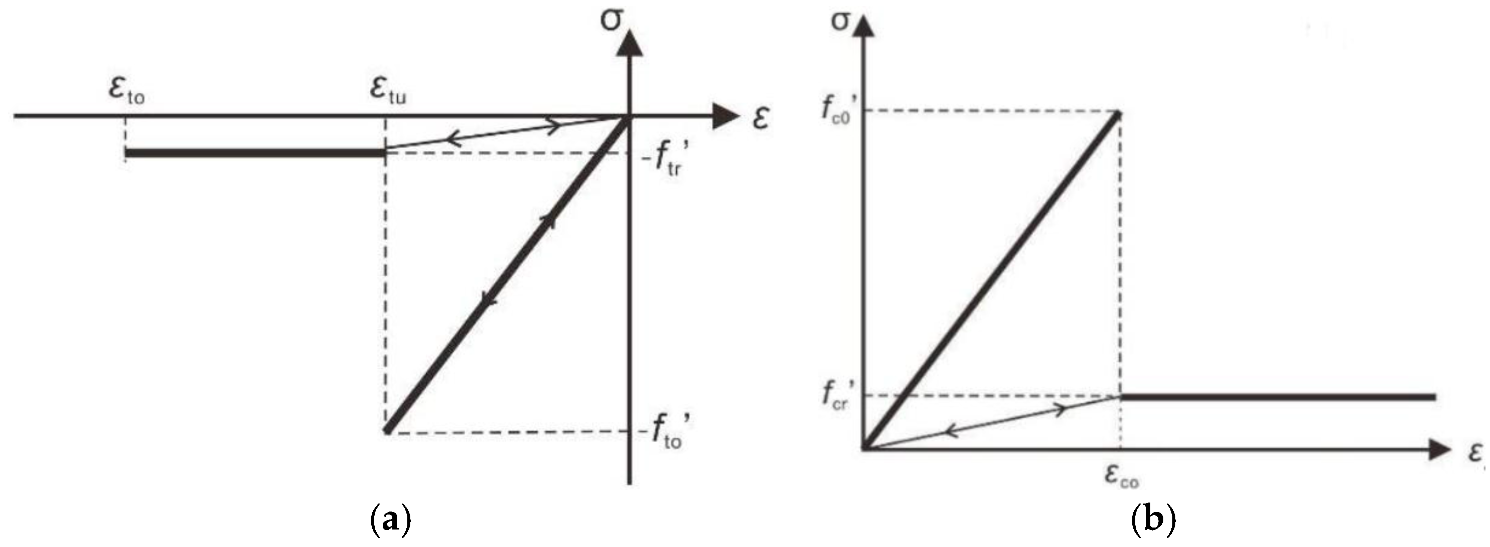
the RFPA-Flow code can simulate non-linear deformation of a quasi-brittle behavior by introducing heterogeneity of rock properties into the model, with an ideal brittle constitutive law for the local material;

(2)

by introducing a deterioration of element parameters after its failure, the RFPA code can simulate strain-softening and discontinuous mechanics problems in a continuum mechanics mode. For heterogeneity, the material properties (failure-strength σ_c and elastic modulus E_c) for elements are randomly distributed throughout the model by following a Weibull distribution:

$$\mathsf{\phi }=\frac{m}{{\mathsf{\sigma }}_0}{\left(\frac{\mathsf{\sigma }}{{\mathsf{\sigma }}_0}\right)}^{m-1}\exp \left[-{\left(\frac{\mathsf{\sigma }}{{\mathsf{\sigma }}_0}\right)}^m\right]$$

(13)

where σ is the element strength; σ₀ is the mean strength of the elements for the specimen; and $\mathsf{\phi }$ is a probability density function. For an elastic modulus, E, the same distribution is used. We define m as the homogeneity index of the rock [23]. According to the definition, a larger m implies a more homogeneous material and vice versa.

3. Numerical Model Setup

3.1. Discrete Fracture Network Realization

In this paper, the main target is the Cretaceous tight sandstone occurring at about 5300–6000 m depth in the northwest Tarim Basin. The rock in the reservoir is composed of siltstones and fine interlayered with thin shales. The average reservoir porosity is about 7% and the average permeability is about 0.07 mD. The gross reservoir thickness is about 180–220 m. Gui et al. [8] have studied the geomechanical properties by a comprehensive use of core data, well log and drilling data, etc. Figure 2a is the statistical result of natural fractures developed in the gas play. The natural fractures observed can be assigned into three groups: The first group is the low-angle fractures (dip < 20°), which could be related to beddings. The second group has intermediate dip angles (25°–55°), which are the major fractures seen in this block and strike at an azimuth of 155 °N. The third group consists of fractures with dip angles 35°–65° and strikes of 355 °N and 100 °N and dip angles 35°–65° and 25°–35°, respectively.

Explicit representation of the DFN with realistic characteristics is thus important in the numerical modeling. DFNs are often characterized by several statistical parameters, among them, fracture orientation distribution, fracture spacing distribution, fracture length distribution and fracture persistence of each fracture set, etc. [3,29,30,31,32]. The combinations of these statistical characteristics that describe the geometrical properties of a DFN defined by the macro-scale connectivity and directional flow preference of the DFN are essential for the fluid transport characterization of an unconventional reservoir. According to the results from core data, well log data and drilling data [8], we developed the corresponding DFN model to represent the three natural fracture groups.

For this study, a DFN generator was developed that was capable of creating a fracture network that satisfied the assigned input statistical characteristics and allowed for the quantitative variation of the studied case. In this paper, the developed DFN models are called the Beacher Model and the Parallel Deterministic Model, respectively. The detailed descriptions of these two DFN models are found as below:

(1)

Beacher DFN model. The Beacher model [33] is a flexible algorithm that can generate complicate joint networks. In this model, the joints are assumed to have finite trace length, which follow some statistical distributions. The centers of the joints are located in space according to a Poisson point process. The orientation of the joints in a Beacher discrete fracture network can either be constant or vary according to an orientation distribution. The number of the joints generated in a Baecher network is controlled by a joint intensity. So as to avoid boundary effects in a specified model region, the Baecher algorithm first increases the region before generating joints. After generating the joints according to the required joint intensity, the algorithm then clips the network with the original bounding region. Joints of the Baecher discrete network fracture generally terminate in intact rock. The main parameters for Baecher DFN model include the joint Orientation, Dip/Dip Direction, Joint Length and Joint Intensity. The Baecher DFN model can be re-generated, using a new sampling of the random variables (e.g., joint orientation, joint length).

(2)

Parallel Deterministic DFN model. The Parallel Deterministic DFN model allows us to define a network of parallel joints with fixed spacing and orientation. In this case, deterministic indicates that the length, spacing, and persistence of the joints are assumed to be constant (i.e., exactly known with no statistical variation). However, the Parallel Deterministic DFN model does allow randomness of the joint location.

3.2. RFPA-Flow Model Setup

According to the DFN generator mentioned above, three DFN groups were generated for the studied case. Figure 2 shows the geometry and the set-up of the simulation model. The orientation of the natural fractures has been converted according to direction of the simulations, the maximum horizontal stress (SHmax). The dimensions of the fractures have been converted by similarity criterion [1,8]. The model represents a 2D horizontal section of a reservoir with a laboratory scale. In the model, the injection is through a vertical wellbore in the center of the model, the injected fluid was imposed on the wellbore at a constant rate. The whole model is composed of 40,000 (200 × 200) identical square elements with dimension of 400 mm × 400 mm. The diameter of the injection hole was 15 mm. As shown in Figure 2c shows the Parallel Deterministic DFN model, which represents the first group natural fractures, and is related to beddings; Figure 2c,d show the Beacher DFN model, which represented the second and third group natural fractures, respectively. For the first group DFN, the joints were generated by the Beacher distribution, and it had an average inclination of 78° with normal distribution, and a standard deviation (std) of 5°. It had a mean length of 60 mm with exponential distribution, relative minimum of 3 mm, and relative maximum of 10 mm. The joint intensity (the number of joint traces per unit area of the trace plane) for the first group was 0.007. For the first group DFN, the joints were generated by the Beacher distribution, and it had an average inclination of −30° with normal distribution, std, of 5°. It had a mean length of 45 mm with exponential distribution, relative minimum of 3 mm, and relative maximum of 5 mm. The joint intensity (the number of joint traces per unit area of the trace plane) for the first group was 0.003. For the first group DFN, it had an average inclination of −20°, the spacing was 50 mm, the length was 200 mm, and persistence (uniform length of intact material between each joint segment.) was 0.9.

The input material mechanical parameters for the numerical model are based on the work by Gui et al. [8], the main parameters used for hydraulic fracturing were obtained by similarity criterion, as is shown in

Table 1. Input material mechanical parameters for the studied numerical model.

Index	Rock Matrix	DFN-1	DFN-2	DFN-3	Unit
Homogeneity index (m)	2	3	3	3	-
Elastic modulus (E0)	34	23	30	30	GPa
Poisson’s ratio (v)	0.22	0.33	0.32	0.31	-
Internal friction angle (φ)	53	30	32	35	°
Compressive strength (σc)	320	150	220	240	MPa
Tensile strength (σt)	32	15	22	24	MPa
Coefficient of residual strength	0.1	0.1	0.1	0.1	-
Permeability coefficient (k0)	0.07	0.12	0.12	0.13	mD
Porosity	0.07	0.17	0.13	0.11	-
Coupling coefficient (β)	0.01	0.01	0.01	0.01	-
Coefficient of pore-water pressure (α)	0.6	0.6	0.6	0.6	-

. For all the SHmax was 21.2 MPa, the simulations, the minimum horizontal stress (SHmin) was 20.5 MPa. The initial pore pressure was set to 16.5 MPa. The slick-water treatment is selected during the simulations, fluid rheology is 1 centipoise (cp). It is noteworthy that the simulation model is based on laboratory scale, not field scale. The reason is that because the calculation for the field scale model was too large, the computation efficiency was extremely low. The connection between the field scale and laboratory scale is due to similarity criterion [34].

3.3. Numerical Experiment Design

The focus of this work is on the numerical investigation of four different variable injection-rate cases, to study and compare the HF and DFN interactions, and to determine the hydraulic fracturing effectiveness and microseismic response for different variable injection-rate technology. A series of comparative studies were performed to establish the effect of variable injection-rate with the same DFN connected configuration, as shown in Figure 2f. Four fluid injection rates (0.15, 0.3, 0.6 and 1.2 mL/s) were applied to the same DFN model at different injection stage. The primary four numerical cases are as following:

Case 1

Fluid injection rate decreases, then increases, and decreases again: 1.2 mL/s → 0.15 mL/s → 0.6 mL/s → 0.3 mL/s;

Case 2

Fluid injection rate decreases, then increases, and decreases again: 0.6 mL/s → 0.3 mL/s →1.2 mL/s → 0.15 mL/s;

Case 3

Fluid injection rate monotonicallydecreases: 1.2 mL/s → 0.6 mL/s → 0.3 mL/s → 0.15 mL/s;

Case 4

Fluid injection rate monotonicallyincreases: 0.15 mL/s → 0.3 mL/s → 0.6 mL/s → 1.2 mL/s.

For the studied case, the total injected fluid is 22.05, 12.5, 31.38, and 11.85 mL. In addition to qualitative evaluation of the simulation results, the model responses are compared in terms of a series of indices that were evaluated during injection. These indices include:

(a)

Injection pressure, defined as the fluid pressure at the injection point;

(b)

Injection rate, defined as the fluid injection rate at different stages;

(c)

Stimulated total interaction area, defined as the interaction area of HF and DFN that has experienced a fluid pressure increase due to injection; and

(d)

Leak off ratio, defined as the total volume of fluid leaked into the DFN model and used in hydraulic fracture generation divided by the total volume of fluid injection.

4. Numerically Simulated Results and Discussion

4.1. General Observations

Figure 3 shows the progressive hydraulic fracturing process for the four variable injection-rate cases. These figures plot the relative magnitude of the pore water pressure field at each fracturing stage (e.g., for Case 1, the critical injection rates are 1.2, 0.15, 0.6 and 0.3 mL/s, respectively). From these simulators, it can be seen that interaction between HF and DFN is different with different variable injection-rate technologies. This results in the different hydraulic fracturing effectiveness, accordingly. From the results of Case 1, no fractures appear at step 5; with the increase of injection pressure at step 20, numerous fractures appear until failure of the model. From the results of Case 2, no fractures appear at step 6; with the increase of injection pressure at step 14, many fractures appear until failure of the model. We can also see that the number of fracture at step 14 is much more than in Case 1 at step 20. From the results of Case 3, at the first hydraulic fracturing stage (step 8), some fractures appear around the injection hole; with the increase of injection pressure, at the end of the second stage (step 20), fractures propagate along the direction SHmax until failure of the model. From the results of Case 4, at the end of the first and second stage (steps 5 and 10), no fractures appear at the injection hole; with the increase of injection pressure, at the end of the third stage (step 14), plenty of fractures appear and propagate almost along the direction of SHmax until failure of the model.

From Figure 3, it can also be seen that the order of hydraulic fracturing effectiveness for the four cases is: Case 4 > Case 2 > Case 1 > Case 3. The effectiveness is the best for Case 4 and is the worst for Case 3. For Case 4, fluid injection rate monotonically increases, which leads to the strong interaction between HF and DFN. However, when fluid injection rate monotonically decreases at each state, the interaction between HF and DFN is the weakest. It was observed that the results of observation, the hydraulic fracturing effectiveness of Case 2 is not bad, and the interaction between HF and DFN becomes stronger at step 18; at the last stage (step 30), the degree of interaction between HF and DFN has not improve much; this phenomenon shows that after step 30, the injected fluid has almost leaked into the already opened fractures. However, for Case 4, the degree of interaction between HF and DFN improves largely from steps 14–20, the injected fluid is used to generate new HF and shear stimulated DFN. The initiation and propagation of fractures is related to the degree of damage at different injection stages for the four cases.

4.2. Microseismic Response

With the RFPA-Flow approach, the number of failed elements and the associated energy can be recorded, which can be treated as indicators of microseismic events during fluid injection. The energy and magnitude is related to the strength of failure elements. Figure 4 shows the magnitudes of the synthetic microseismic moment and the distributions for the DFNs with for the four studied cases. It is noted that because most of the natural fractures are subjected to tensile failure, the released energy is very small, so some microseismic events cannot be recorded during hydraulic fracturing. From these results, the number of microseismic events for Case 4 is the maximum; however, for Case 3 it is the minimum; this phenomenon implies that the fracturing effectiveness is the best for Case 4. We can also see that for Case 4, with the increase of injection rate at each stage, it accumulates the most associated energy with the increase of injection step. The size of the circle indicates the magnitude of the microseismic events, the circle’s diameter for Case 4 is the biggest, and this indicates that the interaction between HF and DFN is the most obvious. For Case 2, the number of microseismic events is more than Case1 and Case 3, but less than Case 4; after step 18, the injected fluid leaks into the already opened fractures. The cumulative acoustic emission (AE) number for the four models is 1048, 4221, 400, and 5403, respectively. From the results of the microseismic events, order of the hydraulic fracturing effectiveness for the studied cases is: Case 4 > Case 2 > Case 1 > Case 3. The complexity of microseismic events was consistent with field observations and suggests an intensive interaction between the created hydraulic fractures and natural fractures. So, it suggests that for the case when injection rate increases monotonically, incremental injection-rate technology has the most obvious hydraulic fracturing effectiveness.

4.3. Hydraulic Fracture and Discrete Fracture Network Interaction

In Figure 3 and Figure 4, the qualitative observations were further studied quantitatively by seeking the evolution of the HF and the DFN interaction area. As no precise criteria for defining the interaction area has been published, a criteria based on a pore pressure change was employed in this work. In this work, the interaction area corresponds to the area marked red color, which is also corresponding to a high leak off region. The pore pressure in this region is the maximum, and the interaction between hydraulic fractures and natural fractures is the most severe. Determination of the area of the “red” region is used the digital image process (DIP) method. The stimulated total interaction area can be obtained from the contour of the simulation results. Figure 5 shows the plots of injection pressure and injection rate against injection step for the studied cases. For each studied case, the pore pressure varies largely at the end of each injection stage. At the end of the fourth injection stage, pore pressure of Case 2 is at a minimum; however, it is a maximum for Case 3. These phenomenon can be interpreted that for Case 2, the injection rate is 0.15 mL/s at the last stage, and in this state, the injected fluid leaks off into the already opened fractures, the injected fluid is not used to generate new hydraulic fractures. For Case 3, although the hydraulic fracturing effectiveness is observed to be the worst from the observation (Figure 3 and Figure 4), the injected fluid is mostly used to drive the propagation of HF; the rock bridges block the fluid into the formations, and leaking off is a minimum for this case. These results indicate that hydraulic fracturing effectiveness is determined by the interaction of HF and DFN, the injected fluid is partly used to drive the propagation of HF and partly used to leak off into DFN to stimulate natural fractures.

Figure 6 shows the total interaction area of HF and DFN against injection step for the four studied cases. For the four studied cases, when injection pressure reaches the crack initiation pressure (defined as the pressure when element in the model begins to failure), fractures appear and the total interaction area increases with the increase of injection step. But the step of crack initiation is not the same for these studied cases; also, the injection rate corresponding to the crack initiation step is not the same. This phenomenon can be better interpreted by evaluating the pressure contour in Figure 2. With different variable injection-rate technologies, the damage elements are different for the studied cases. As shown in Figure 6, the interaction total area is different at each crack initiation step; it is a maximum for Case 2 and a minimum for Case 3. This result indicates that the number of damaged elements in the four cases is different for each different variable injection-rate technology before the injection pressure reaches the crack initiation pressure. The total interaction area increases with the increase of injection step, but the incremental rate is different. For Case 4, the incremental rate is the most obvious; however, for Case 2, the incremental rate is the least obvious. This implies that the hydraulic fracturing effectiveness is the best for Case 4.

4.4. Hydraulic Fracturing Effectiveness Evaluation

In this study, two indices were selected to evaluate the hydraulic fracturing effectiveness of the fracturing network with different cases. They are the stimulated total interaction area between HF and DFN and the leakoff ratio (as mentioned above). Figure 7 shows the results of a stimulated total interaction area at each variable injection-rate stage. From the simulation results, that the total interaction area of Case 4 is the maximum, so the hydraulic fracturing effectiveness is the best. The variable injection rate technology is helpful for improving the complexity of the fracture network. The results in this paper are consistent with the results drawn by Hou et al. [22], who studied the hydraulic fracture propagation behaviors in shale block using tri-axial fracturing test systems. After studying the effect of injection rate on fracturing effectiveness, he concluded that variable flow rate increases the possibility that the hydraulic fracture communicates with bedding planes and natural fractures. If the development characteristics of natural fracture in shale reservoir are well understood, variable flow rate fracturing could be attempted at proper timing [22]. In this work, at initial fracturing stages, the fracturing effectiveness for Case 4 is not obvious, and the effectiveness is poor than Cases 1–3. After the third stage, the hydraulic fracturing effectiveness for Case 4 significantly improves. The is due to the fluid injection mode; for Case 4, the injection rate is lower at the initial stage, and the internal micro-fractures gradually accumulate gradually during this process, when it reaches stage 3, the number of micro-fractures is a maximum, then the remaining injection rate increases and leads to the dynamic propagation of fractures, such as branching and turning, etc.

Another index that can be used to evaluate the overall effect of variable injection-rate technology on hydraulic fracturing effectiveness is the leak off ratio, which is defined as the ratio of the injected fluid leaked into the DFN and used in hydraulic fracture generation to the total volume of fluid injection. For the studied model, the fluid injection mode adopts flow rate, unit is “mL/s”. In RFPA-Flow software, we can also select the pressure control model, unit is “MPa/step”. For the same pump pressure-injection step curves, there exists relationship between them. By the change of the pump pressure, we can calculate the change of injected fluid. The volume of injected fluid can be obtained by injection steps multiplied by injection rate. When the fluid leaks off to fractures, the pore pressure will drop, the part of drop is the fluid leaked into the DFN model. From Figure 8, the leak-off ratio for Case 4 is greater than the other three cases, this also indicates that the hydraulic fracturing effectiveness is the best among the four cases. For Case 3, the leakoff ratio is a minimum, this indicates that interaction between HF and DFN is least obvious; little injected fluid was used to generate new hydraulic fractures; as is generally observed in Figure 2, the injected fluid was used to stimulated DFN only. The variable injection rate case is shown to significantly affect the leak-off ratio for natural fractured formations. For the same case at each hydraulic fracturing stage, the hydraulic fracturing effectiveness increases with fluid leaking off to the model. The oscillation in the leakoff ratio curve is due to the initiation and propagation of HF, which is due to the reaction of natural fractures. For example, the high point may be correspond to times when a new natural fracture is connected to the HF during the HF propagation process.

Despite the recent success in shale gas development, the cost of hydraulic fracturing treatment remains very high. Therefore, optimization of hydraulic fracture treatment design is extremely urgent. During field hydraulic fracturing, what we are concerned with most is the fluid volume injected into the shale plays; the injected volume determines the input cost. It is desirable to inject the minimum fluid volume to obtain the maximum gas production. The total injection volume injected to the DFN model is calculated as the sum of fluid volume at each state, which is expressed as below:

$$InjectionVolume={\displaystyle \sum _1^{n}I{R}_1\times }{T}_i+{\displaystyle \sum _1^{n}I{R}_2\times }{T}_i+{\displaystyle \sum _1^{n}I{R}_3\times }{T}_i+{\displaystyle \sum _1^{n}I{R}_4\times }{T}_i$$

(14)

where IR₁, IR₂, IR₃, and IR₄, correspond to the injection rate at each state to the studied case, respectively; T_i is the injection step.

According to Equation (14), for the studied cases, Case 4 has the minimum injected volume; however, Case 3 has the maximum injected volume. The injected volume of Case 2 is closed to Case 4, 12.5 mL versus 11.85 mL. However, after the third stage for Case 2, the injected fluid mostly leaks into the opened fractures. And more fracturing fractures cannot form in the fourth stage. Case 2 also implies that relative lower injection rates at the initial stages is helpful, and after many under-fracturing points have formed in shale, and then applying high injection rate is beneficial. The combination with the analysis results above, hydraulic fracturing effectiveness of Case 4 is the best; therefore, the variable injection-rate technology of Case 4 is most suitable for hydraulic fracturing.

4.5. Mechanism of Variable Injection-Rate Technology

The variable injection-rate hydraulic fracturing technology is different from traditional technology. The injection rate is variable at different stages during hydraulic fracturing, the key point of this technology is the occasional selection of the variable injection-rate and injection-rate range. In this study, the selection of the variable occasions is according to the real time dynamic monitor of the simulators. Taking Case 4 for example, Figure 9 shows the maximum shear stress contours at different injection stages. At step 5 (Figure 10a), some damaged points appear around the wellbore. At step 10 (Figure 10b), the number of damaged points appears that appear around the wellbore increases to a large extent. At step 14 (Figure 10c), the number of under-fracturing points that appear around the wellbore surges. Therefore, steps 5, 10, and 14 are selected to change the injection rate, four injection stages are divided by the three different injection rates.

The mechanism of the variable injection rate technology can be interpreted by a mechanical damage process of the internal elements in the DFN model. It is well-known that the brittleness of shale is high, at the initial stage, a relatively lower injection rate is used during hydraulic fracturing, water pore pressure is built and held gradually, the natural fractures around the wellbore could be damaged with the increase of pore pressure, and some damaged points are faced with failure. Before the pore pressure reaches the initiation pressure, numerous weak cemented micro-fractures appear in the shale under tensile stress. The micro-fractures may be located around the wellbore or far-away from the wellbore. The presentation of the micro-fractures influences the propagation of hydraulic fractures and the scale of the fracturing network. These micro-fractures are facing tensile and shear failure; we call these micro-fractures as the under-fracturing point. Before the initiation of HF, lots of micro-fractures have existed in shale. If the fractures are forced to branch and turn, it should have much greater energy around the location of the hydraulic fractures. Therefore, the pump pressure should be enlarged by increasing the injection rate. With the increase of injection rate, the total SRV can be obtained.

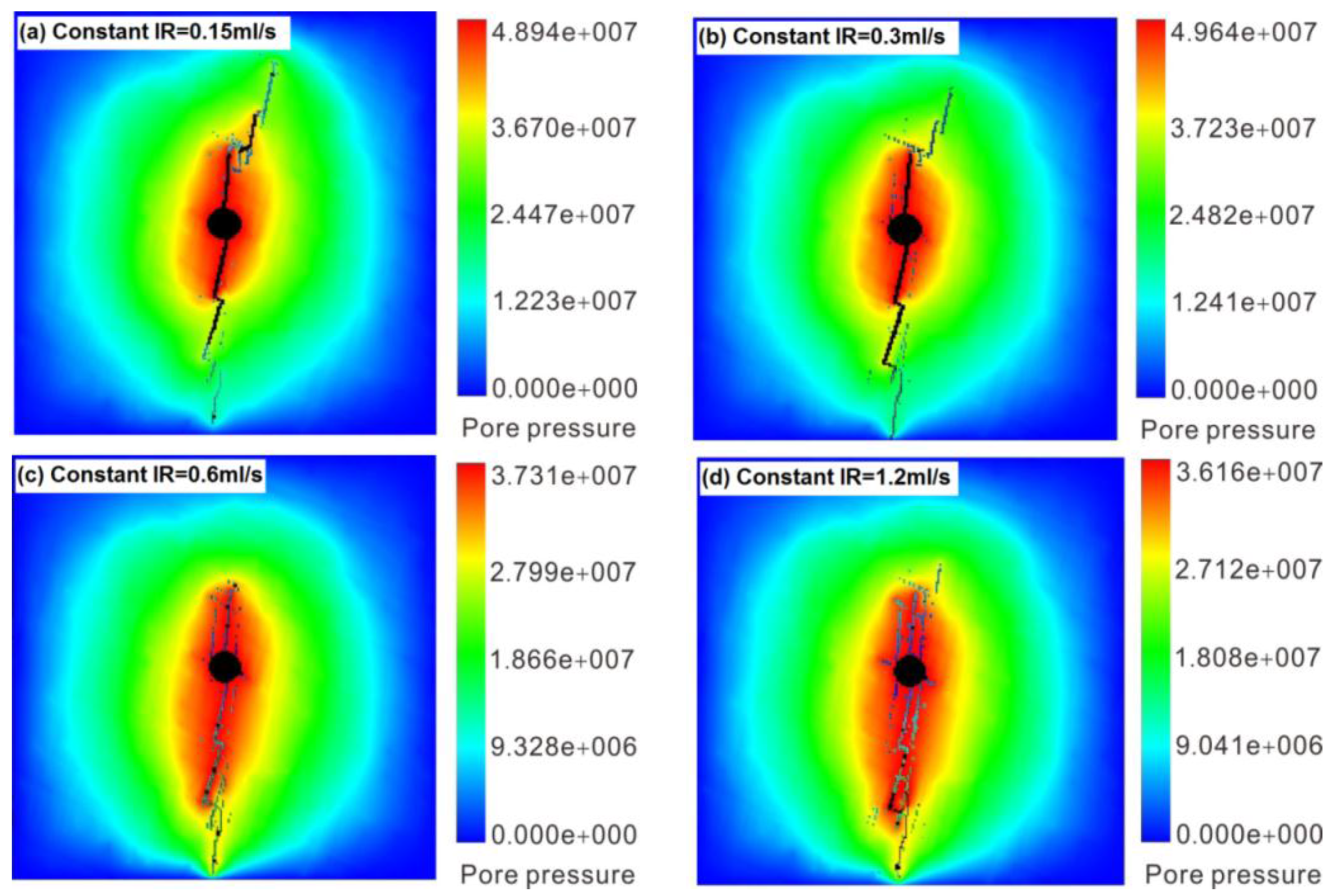
4.6. Comparison with Constant Injection Rate Technology

In this section, the constant injection-rate technology is used during hydraulic fracturing; hydraulic fracturing effectiveness is compared with the variable injection-rate cases. Using the same model (Figure 1f), four injection rates (i.e., 0.15, 0.3, 0.6 and 1.2 mL/s) were applied to the two-dimensional DFN model, respectively. As is shown in Figure 10, the hydraulic fracturing effectiveness for the models at constant injection rate of 0.15, 0.3 and 0.6 mL/s is worse than the variable injection-rate cases studied above. Only the constant injection rate of 1.2 mL/s has better hydraulic fracturing effectiveness than Case 3 studied above. Overall, the results of constant injection rate technology are worse than Case 4 studied above. And, the injected fluid volume of the four constant cases is 22.5, 30, 18.6 and 19.2 mL, respectively. Compared with the cases of variable injection rate simulations, volume of the constant case is greater than the fourth case of variable injection rate solution (injected volume of is 11.85 mL).

The variable injection-rate technology compared with the constant injection-rate technology indicates that it can lead to the formation of a complex fracturing network. Variable injection-rate technology not only overcomes the disadvantage of the small-pump supply, but also the fracturing fluid cannot be leaked into the shale stratum completely. This result is consistent with the studied of King [1], Beugelsdijk et al. [9] and Nagel et al. [10]. Although low injection rate in shales have been successful in opening natural fractures, low injection rates have not been successful in developing lasing gas rates even with large fracturing volumes [18]. The pressure pulse can be formed in naturally fractured formations by the variable injection-rate technology; the natural fractures are easy to be stimulated, and interaction between shear stimulated natural fractures and hydraulic fractures result in the maximum fracturing network. For different reservoirs, the key of variable injection-rate technology is to determine the occasion of changing the injection-rate, and the range of injection-rate. Fortunately, these two problems can be solved by simulation test ahead of time.

5. Conclusions

In this study, the variable injection-rate technology was numerically investigated for a naturally fractured reservoir, the Tarim Basin in China. Four primary cases were conduct to study the HF and DFN interactions, propagation, microseismic response and hydraulic fracturing effectiveness. Also, another four constant injection-rate cases were conducted to compare with the variable flow rate technology. The designed numerical simulations confirm that the variable flow rate technology is expected to instruct hydraulic fracturing treatment for shale reservoirs. The main conclusions from this study are as follows:

(1)

The fluid injection rate is critical to the overall response of the formation in hydraulic fracturing. This work suggests that variable injection-rate plays a crucial role in hydraulic fracturing effectiveness for unconventional tight gas developments, and variable injection-rate will play a significant role in optimizing treating pressures, the created microseismicity and corresponding SRV, and well production.

(2)

The hydraulic fracturing effectiveness with variable flow rate technology is generally better than those of constant injection rate technology. Of the four studied cases, the effectiveness of the injection rate increasing at each stage is the best.

(3)

The mechanism of the variable injection-rate technology is the initiation of numerous under-fracturing points at different injection stages, branching and accumulation of micro-fractures, and the formation of a fracturing network. At the initial stage, many damaged elements (under-fracturing points) appear around the wellbore with the increase of pore pressure. Furthermore, the sudden increase of injection rate drives the dynamic propagation of hydraulic fractures along many branching fracturing points.

(4)

More natural fractures can be shearing stimulated by variable injection-rate technology, which is helpful in developing a complex fracturing network. Selecting the reasonable variable injection-rate occasion and injection-rate range is the key to this technology. However, these two problems can be solved by simulation tests.

References

1. King, G.E. Thirty Years of Gas Shale Fracturing: What Have We Learned? In Proceedings of the SPE Annual Technical Conference and Exhibition, Florence, Italy, 19–22 September 2010.
2. Jeffrey, R.G.; Zhang, X.; Bunger, A.P. Hydraulic Fracturing of Naturally Fractured Reservoirs. In Proceedings of the 35th Workshop on Geothermal Reservoir Engineering, Stanford, CA, USA, 1–3 February 2010.
3. Wang, Y.; Li, X.; Zhou, R.Q.; Tang, C.A. Numerical evaluation of the shear stimulation effect in naturally fractured formations. Sci. China Earth Sci. 2016, 59, 371–383. [Google Scholar] [CrossRef]
4. Behnia, M.; Goshtasbi, K.; Marji, M.F.; Golshani, A. Numerical simulation of interaction between hydraulic and natural fractures in discontinuous media. Acta Geotech. 2015, 10, 533–546. [Google Scholar] [CrossRef]
5. Warpinski, N.R.; Waltman, C.K.; Du, J.; Ma, Q. Anisotropy Effects in Microseismic Monitoring. In Proceedings of the SPE Annual Meeting and Exhibition, New Orleans, LA, USA, 4–7 October 2009.
6. Wang, Y.; Li, X.; Zhou, R.Q.; Zheng, B.; Zhang, B.; Wu, Y.F. Numerical evaluation of the effect of fracture network connectivity in naturally fractured shale based on FSD model. Sci. China. Earth. Sci. 2016, 59, 626–639. [Google Scholar] [CrossRef]
7. Gale, J.F.W.; Read, J.M.; Holder, J. Natural fractures in the Barnett shale and their importance for hydraulic fracture treatments. AAPG Bull. 2007, 91, 603–622. [Google Scholar] [CrossRef]
8. Gui, F.; Rahman, K.; Moos, D. Optimizing Hydraulic Fracturing Treatment Integrating Geomechanical Analysis and Reservoir Simulation for a Fractured Tight Gas Reservoir, Tarim Basin, China. In Proceedings of the ISRM International Conference for Effective and Sustainable Hydraulic Fracturing, Brisbane, Australia, 20–22 May 2013.
9. Beugelsdijk, L.J.L.; De Pater, C.J.; Sato, K. Experimental Hydraulic Fracture Propagation in a Multi-Fractured Medium. In Proceedings of the SPE Asia Pacific Conference in Integrated Modeling for Asset Management, Yokohama, Japan, 25–26 April 2000.
10. Gil, I.; Nagel, N.; Sanchez-Nagel, M. The Effect of Operational Parameters on Hydraulic Fracture Propagation in Naturally Fractured Reservoirs—Getting Control of the Fracture Optimization Process. In Proceedings of the 45th U.S. Rock Mechanics/Geomechanics Symposium, San Francisco, CA, USA, 26–29 June 2011.
11. Nagel, N.; Gil, I.; Sanchez-Nagel, M.; Damjanac, B. Simulating Hydraulic Fracturing in Real Fractured Rock—Overcoming the Limits of Pseudo 3D Models. In Proceedings of the SPE Hydraulic Fracturing Technology Conference, Woodlands, TX, USA, 24–26 January 2011.
12. Kresse, O.; Cohen, C.; Weng, X.; Wu, R.; Gu, H. Numerical Modeling of Hydraulic Fracturing in Naturally Fractured Formations. In Proceedings of the 45th U.S. Rock Mechanics/Geomechanics Symposium, San Francisco, CA, USA, 26–29 June 2011.
13. Overbey, W.K.; Yost, A.B., II; Wilkins, D.A. Inducing Multiple Hydraulic Fractures from a Horizontal Wellbore. In Proceedings of the SPE Annual Technical Conference and Exhibition, Houston, TX, USA, 2–5 October 1988.
14. Yost, A.B.; Overbey, W.K.; Wilkins, D.A.; Locke, C.D. Hydraulic Fracturing of a Horizontal Well in a Naturally Fractured Reservoir, Gas Study for Multiple Fracture Design. In Proceedings of the SPE Gas Technology Symposium, Dallas, TX, USA, 13–15 June 1988.
15. Yost, A.B.; Overby, W.K., Jr. Production and Stimulation Analysis of Multiple Hydraulic Fracturing of a 2,000-ft Horizontal Well. In Proceedings of the SPE Gas Technology Symposium, Dallas, TX, USA, 7–9 June 1989.
16. Nearing, T.R.; Startzman, R.A. Shale Well Productivity. In Proceedings of the SPE Eastern Regional Meeting, Charleston, WV, USA, 1–4 November 1988.
17. Gale, J.F.W.; Laubach, S.E.; Olson, J.E.; Eichhubl, P.; Fall, A. Natural fractures in shale: A review and new observations. AAPG Bull. 2014, 98, 2165–2216. [Google Scholar] [CrossRef]
18. Warpinski, N.R.; Mayerhofer, M.J.; Vincent, M.C.; Cipolla, C.L.; Lolon, E.P. Stimulating unconventional reservoirs: Maximizing network growth while optimizing fracture conductivity. J. Can. Pet. Technol. 2008, 48, 39–51. [Google Scholar] [CrossRef]
19. Pacheco, K.W. Petroleum potential for the Gothic Shale, Paradox Formation in the Ute Mountain Ute Reservation, Colorado and New Mexico. Master’s Thesis, Colorado School of Mines, Golden, CO, USA, 16–17 December 2007. [Google Scholar]
20. Paktinat, J.; O'Neil, B.J.; Tulissi, M.G. Case Studies: Impact of High Salt Tolerant Friction Reducers on Freshwater Conversation in Canadian Shale Fracturing Treatments. In Proceedings of the Canadian Unconventional Resources Conference, Calgary, AB, Canada, 15–17 November 2011.
21. King, G.E.; Haile, L.; Shuss, J.A.; Dobkins, T. Increasing Fracture Path Complexity and Controlling Downward Fracture Growth in the Barnett Shale. In Proceedings of the SPE Shale Gas Production Conference, Fort Worth, TX, USA, 16–18 November 2008.
22. Hou, B.; Chen, M.; Li, Z.M. Propagation area evaluation of hydraulic fracture networks in shale gas reservoirs. Pet. Explor. Dev. 2014, 41, 833–838. [Google Scholar] [CrossRef]
23. Tang, C.A.; Tham, L.G.; Lee, P.K.K.; Yang, T.H.; Li, L.C. Coupled analysis of flow, stress and damage (FSD) in rock failure. Int. J. Rock Mech. Min. Sci. 2002, 39, 477–489. [Google Scholar] [CrossRef]
24. Wang, S.Y.; Sun, L.; Au, A.S.K.; Yang, T.H.; Tang, C.A. 2D-numerical analysis of hydraulic fracturing in heterogeneous geo-materials. Constr. Build. Mater. 2009, 23, 2196–2206. [Google Scholar] [CrossRef]
25. Wang, S.Y.; Sloan, S.W.; Fityus, S.G.; Griffiths, D.V.; Tang, C.A. Numerical Modeling of Pore Pressure Influence on Fracture Evolution in Brittle Heterogeneous Rocks. Rock Mech. Rock Eng. 2013, 46, 1165–1182. [Google Scholar] [CrossRef]
26. Biot, M.A. General theory of three-dimensional consolidation. J. Appl. Phys. 1941, 12, 155–164. [Google Scholar] [CrossRef]
27. Thallak, S.; Rothenbury, L.; Dusseault, M. Simulation of Multiple Hydraulic Fractures in a Discrete Element System. In Proceedings of the 32nd U.S. Symposium on Rock Mechanics (USRMS), Norman, OK, USA, 10–12 July 1991.
28. Noghabai, K. Discrete versus smeared versus element-embedded crack models on ring problem. J. Eng. Mech. 1999, 125, 307–315. [Google Scholar] [CrossRef]
29. Engelder, T.; Lash, G.G. Marcellus Shale Play’s Vast Resource Potential Creating Stir in Appalachia, the American Oil and Gas Reporter. May 2008. Available online: http://www.aogr.com/magazine/cover-story/marcellus-shale-plays-vast-resource-potential-creating-stir-in-appalachia (accessed on 23 May 2008).
30. Olson, J.E. Sublinear scaling of fracture aperture versus length: An exception to the rule? J. Geophys. Res. Solid Earth 2003, 108. [Google Scholar] [CrossRef]
31. Olson, J.E. Predicting fracture swarms—the influence of subcritical crack growth and the crack-tip process zone on joint spacing in rock. Geol. Soc. 2004, 231, 73–88. [Google Scholar] [CrossRef]
32. Nagel, N.B.; Sanchez-Nagel, M.A.; Zhang, F. Coupled numerical evaluations of the geomechanical interactions between a hydraulic fracture stimulation and a natural fracture system in shale formations. Rock Mech. Rock Eng. 2013, 46, 581–609. [Google Scholar] [CrossRef]
33. Baecher, G.B.; Lanne, N.A.; Einstein, H.H. Statistical Description of Rock Properties and Sampling. In Proceedings of the 18th U.S. Symposium on Rock Mechanics, Golden, CO, USA, 22–24 June 1977.
34. Liu, G.H.; Pang, F.; Chen, Z.X. Fracture simulation tests. J. Chin. Univ. Pet. 2000, 24, 23–31. (In Chinese) [Google Scholar]
Figure 1. Elastic-brittle damage constitutive law of element subject to uniaxial stress: (a) the case under uniaxial tensile stress; (b) the case under uniaxial compressive stress.
Energies 09 00414 g001
Figure 2. Numerical model setup: (a) statistical results of nature fractures by Gui et al. [8]; (b) the microscopic heterogeneity background model, the failure-strength and elastic modulus obeys Weibull distribution; (c)–(e) the developed discrete fracture network (DFN) model; (c,d) are the Beacher Model; and (e) is the Parallel Deterministic Model; (f) the calculation model in this paper, considering the macroscopic and microscopic heterogeneity characteristics, simultaneously.
Energies 09 00414 g002
Figure 3. General observations of the fracking process for the four cases at each hydraulic fracturing stage (Color shadow indicate relative magnitude of the pore water pressure field).
Energies 09 00414 g003
Figure 4. The synthetic microseismic events at different injection rate for the four studied variable injection rate cases. The synthetic microseismic events are colored by red when elements are compressive-shear failure and white when tensile failure. The size of circle indicates magnitude of microseismic events (Note that: element whose failure energy is relative small, microseismic sign is not brought out).
Energies 09 00414 g004
Figure 5. Relationship of injection pressure, injection step and injection rate for the studied case: (a) variation of injection rate is 1.2 mL/s → 0.15 mL/s → 0.6 mL/s → 0.3 mL/s; (b) variation of injection rate is 0.6 mL/s → 0.3 mL/s → 1.2 mL/s → 0.15 mL/s; (c) variation of injection rate is 1.2 mL/s → 0.6 mL/s →0.3 mL/s → 0.15 mL/s; and (d) variation of injection rate is 0.15 mL/s → 0.3 mL/s → 0.6 mL/s → 1.2 mL/s).
Energies 09 00414 g005
Figure 6. Relationship between stimulated total interaction area and injection step for the four studied cases: (a) variation of injection rate is 1.2 mL/s → 0.15 mL/s → 0.6 mL/s → 0.3 mL/s; (b) variation of injection rate is 0.6 mL/s → 0.3 mL/s → 1.2 mL/s → 0.15 mL/s; (c) variation of injection rate is 1.2 mL/s → 0.6 mL/s → 0.3 mL/s → 0.15 mL/s; and (d) variation of injection rate is 0.15 mL/s → 0.3 mL/s → 0.6 mL/s → 1.2 mL/s).
Energies 09 00414 g006
Figure 7. Comparison of total interaction area for different variable injection rate cases.
Energies 09 00414 g007
Figure 8. Comparison of leak-off ratio for different variable injection rate cases.
Energies 09 00414 g008
Figure 9. The selection occasions of variable injection-rate technology for Case 4: (a) at step of 5, a few under fracturing points appear; (b) at step of 10, under-fracturing points increases gradually; and (c) at step of 14, the under-fracturing points surges).
Energies 09 00414 g009
Figure 10. General observations of the hydraulic fracturing process for constant injection rate cases (Color shadow indicate relative magnitude of the pore water pressure field) at the constant injection rate: (a) 0.15 mL/s; (b) 0.3 mL/s; (c) 0.6 mL/s; and (d) 1.2 mL/s.
Energies 09 00414 g010