Dynamic Stall Control on the Wind Turbine Airfoil via a Co-Flow Jet

Abstract

Dynamic stall control of a S809 airfoil is numerically investigated by implementing a co-flow jet (CFJ). The numerical methods of the solver are validated by comparing results with the baseline experiment as well as a NACA 6415-based CFJ experiment, showing good agreement in both static and dynamic characteristics. The CFJ airfoil with inactive jet is simulated to study the impact that the jet channel imposes upon the dynamic characteristics. It is shown that the presence of a long jet channel could cause a negative effect of decreasing lift and increasing drag, leading to fluctuating extreme loads in terms of drag and moment. The main focus of the present research is the investigation of the dynamic characteristics of the CFJ airfoil with three different jet momentum coefficients, which are compared with the baseline, giving encouraging results. Dynamic stall can be greatly suppressed, showing a very good control performance of significantly increased lift and reduced drag and moment. Analysis of the amplitude of variation in the aerodynamic coefficients indicates that the fluctuating extreme aerodynamic loads are significantly alleviated, which is conducive to structural reliability and improved life cycle. The energy consumption analysis shows that the CFJ concept is applicable and economical in controlling dynamic stall.

1. Introduction

The depletion of fossil-fuel reserves, stricter environmental regulations and the world’s ever-growing energy demand have greatly promoted the usage of alternative renewable energy sources. Among the various renewable energy alternatives, wind energy is one of the most promising and the fastest growing installed alternative-energy production technology due to its wide availability [1]. In the Half Year Report of World Wind Energy Association [2], it was reported that the growth of the wind energy industry will continue with the rapid increase in energy demand, therefore more efforts are still needed to increase the efficiency of wind energy generation in order to keep wind energy economically competitive compared with traditional fossil fuels and other renewable energy sources such as hydroelectric energy, solar energy and bio-energy.

Two factors that affect the cost of wind energy are lifetime energy capture and maintenance cost. Therefore, since the beginning of the commercial wind industry, the rotor diameter and turbine size have gradually increased in order to capture more energy during the lifetime. As turbines grow in size, the structural and fatigue loads become more noticeable. The extreme structural and fatigue loads are important factors in turbine design and most of these loads result from the dynamic stall. A dynamic stall phenomenon takes place when the wind turbine blade section is subjected to unsteady variation of angle of attack. Due to the complicated atmospheric environment at wind farms, wind turbine blades usually experience adverse conditions under which the local angle of attack of a particular blade section will vary with time, including ground boundary layer effects, horizontal or vertical wind shear, tower shadowing, yaw and tilt misalignment, and unsteady inflow due to atmospheric turbulence or wake from other turbines. All these conditions can give rise to the dynamic stall phenomenon. The unsteady aerodynamic load produced by dynamic stall is also a main source of the vibration [3] and aero-acoustic noise [4]. With increasing deployment, more wind turbines will be located within residential areas, where the aerodynamic noise emitted by the rotors may have a negative impact on the comfort of living in the vicinity. To minimize these factors, reduce maintenance costs, prolong the turbine lifetime and reduce noise level, one effective way is to explore effective flow control methods, passive or active, to alleviate the fluctuations of aerodynamic loads. On the other hand, wind farms in natural conditions may frequently experience adverse working conditions where the wind speed is very low and hence conventional wind turbines generate little or no usable power. This issue has limited the deployment of wind turbines to relatively few sites where favorable wind conditions exist. Therefore, there is a demand to develop effective flow control methods which can significantly increase the lift of the blade at low wind speeds and allow the turbine to cut-in earlier and capture additional energy. Hence, for a flow control method, it is important to provide the blade with both, good static and dynamic, aerodynamic perofmance.

Various flow control methods have been investigated to enhance wind turbine blade performance, including trailing edge flaps [5], microtabs [6,7], vortex generators [8], blowing jets [9,10], circulation control [11], Gurney flaps [11], synthetic jets [12], and plasma actuators [13]. Hanns et al. [10] carried out an experimental study to explore constant blowing as a flow control concept for wind turbine blades. Their results showed that control from the leading-edge slot had a significant potential for load control applications, while control from the mid-chord slot significantly enhanced lift at pre-stall angles of attack but was ineffective for suppressing leading-edge stall. Tongchitpakdee et al. [11] studied and compared the static aerodynamic performances of a wind turbine rotor equipped with trailing-edge blowing and Gurney flaps. The results indicated that for attached flow conditions, trailing-edge blowing and Gurney flap both can produce a net increase in power generation compared with the baseline turbine rotor. However, the results also indicated that at high-wind speed conditions where the flow separates, the trailing-edge blowing and the Gurney flap both became ineffective in increasing the power output. Yen and Ahmed [12] implemented synthetic jets to study the wind turbine dynamic stall control and demonstrated that synthetic jets could improve low speed vertical-axis wind turbine performance but without substantially alleviating stall separation. Greenblatt et al. [13] experimentally measured the effects of plasma pulsation on dynamic stall control on the upwind half of a turbine and also limited phase-locked particle image velocimetry measurements were performed under baseline as well as two controlled conditions. It was found that at lower maximum angles of attack, the effect of pulsations on the dynamic stall was greater, but separation was not fully controlled, and the power required to drive the actuators was significantly larger than the resulting turbine power increase.

Zha et al. [14,15,16,17,18,19,20] have developed a new flow control method by implementing a co-flow jet (CFJ) on the suction surface, which has been proved an effective way to significantly increase lift, stall margin and drag reduction for stationary airfoils and enhance the performance of pitching airfoils in the aircraft research field. The working mechanism of a CFJ is different from the conventional circulation control which relies on large-radius leading edge or trailing edge to induce the Coanda effect and enhance circulation. The CFJ relies on the jet mixing with the main flow to energize the main flow and overcome the adverse pressure gradient. Moreover, the jet suction effect near the suction slot further enhances flow stability to remain attached to the surface at high angles of attack (AoA), thus inducing much higher circulation than conventional circulation control without jet suction. In a previous study, Xu et al. [21] introduced this concept to wind turbine airfoil application, focusing on the static performance with active as well as inactive CFJ. The results showed that steady co-flow jet had a great positive effect in lift enhancement, stall margin expansion, and drag reduction. For cases with jet momentum coefficients larger than 0.12, the total drag even became negative due to the jet reaction forces.

In the present study, the CFJ concept is extended to the dynamic stall control on a wind turbine airfoil. The primary purpose is to investigate the dynamic performance of the CFJ in suppressing wind turbine airfoil dynamic stall and consequently alleviating fluctuating aerodynamic loads. Energy consumed by the CFJ pump is analyzed and compared with the amount of gained energy to assess the economy of implementing the CFJ on the wind turbine to control dynamic stall.

2. Design of the CFJ Airfoil

The NREL S809 wind turbine airfoil is used in the present study as the baseline and its detailed parameters are given in [22]. The corresponding CFJ conceptual airfoil is shown in Figure 1, with an injection slot near the leading edge and a suction slot near the trailing edge on the airfoil suction surface. These slots are formed by translating downward a portion of suction surface, giving rise to the presence of a jet channel. When the co-flow jet is activated, a jet is injected tangentially into the main flow, and a same amount of mass flow is sucked into the suction slot, forming a closed-loop jet circuit. A pump can be used to power the co-flow jet flow. By using a closed-loop jet recirculation, the flow attachment on the suction surface will be greatly strengthened, allowing an attractive ability to resist severe adverse pressure gradients at high angles of attack. The source of jet flow is provided by sucking an equal amount of flow mass from the suction slot rather than the engine, which makes the co-flow jet a zero net mass flow.

The computational model of S809 CFJ airfoil is shown in Figure 2a, which includes the cavities of injection and suction in order to make the simulation more realistic. The location of injection slot AC is set at 6.0%c from the leading edge, perpendicular to the local surface with a height of 0.65%c. The location of suction slot BD is set at 20.0%c from the trailing edge, perpendicular to the local surface with a height of 1.38%c. To ensure that the jet is tangential to the surface, a jet channel linking the injection and suction slots is carefully designed by translating downward and slightly rotating the portion AB of the baseline suction surface to the targeted location CD. For the case of inactivated co-flow jet, there is nearly no mass flow through the slots, the high-pressure and low-pressure cavities are excluded for simplicity, as shown in Figure 2b.

3. Methodology

3.1. Numerical Methods

The unsteady Reynolds-Averaged Navier-Stokes equations and Spalart-Allmaras one-equation turbulence model are used in the present in-house code to carry out the numerical study. More details about the governing equations and boundary conditions can be found in [21]. The dual-time stepping method [23] is adopted to advance the time-accuracy solution with pseudo time marching by means of the LU-SGS method [24]. The Roe scheme [25] with a third order MUSCL reconstruction [26] is used to discretize the inviscid fluxes and second central differencing is used for computing the viscous fluxes. OpenMP parallel computing technique [27] is applied to accelerate the simulation.

The inflow and outflow specified at the far-field boundary are based on the characteristics of the flow. For the inlet and exit boundaries, EF and GH, in the high-pressure cavity and low-pressure cavity shown in Figure 2a, the flow conditions are defined in different ways in order to easily implement the CFJ concept. At the inlet boundary EF, the total pressure P_t, total temperature T_t, flow angle α are specified and inflow velocity u is extrapolated from the interior. At the exit boundary GH, the static pressure P_s is specified, and three primitive flow variables u, v and ρ are extrapolated from the interior domain. In the simulation, the total pressure P_t at boundary EF and static pressure P_s at boundary GH are subject to change during the numerical iteration until the desired jet momentum coefficient is achieved at both inlet EF and outlet GH. The solid surface of airfoil and the cavities are defined as non-slip wall boundaries. Density and pressure on the surface are obtained by extrapolation from the interior solution. For the jet-off case, the jet slots AC and BD are assumed to be wall boundaries, and the high-pressure and low-pressure cavities are not included in the computation.

3.2. Pitch Oscillation Motion and Relevant Parameters

The present study investigates the unsteady aerodynamic characteristics of the NREL S809 baseline and CFJ airfoils undergoing sinusoidal pitch oscillations about the quarter chord point with various jet momentum coefficients. The pitch oscillation motion of an airfoil can be described in a sine-wave form expression which is defined in terms of the instantaneous angle of attack by:

$$\alpha (t)={\alpha }_0+{\alpha }_1\sin (\omega t)$$

(1)

where α₀ and α₁ are the mean angle and pitch oscillation amplitude respectively. $\omega =2\pi f$, with f being the frequency of the oscillation. For oscillating airfoils, the reduced frequency κ is usually used to describe the unsteady motion, which is defined as:

$$\kappa =\frac{\omega c}{2V_{\infty }}$$

(2)

where c is the chord length, and V_∞ is the velocity of the free stream. This parameter represents the interaction between the oscillation motion about pitch axis and the main flow in the chord-wise direction. The magnitude of the parameter reflects the degree of the impact that the oscillation motion imposes upon the main flow.

3.3. Relevant Parameters in CFJ Airfoil Simulation

The implementation of a co-flow jet is usually characterized by a similarity parameter C_μ, known as the momentum coefficient, which is defined as:

$$C_{\mu }=\frac{{\dot{m}}_j{V}_j}{0.5{\rho }_{\infty }{V}_{\infty }^{2}S}$$

(3)

where ${\dot{m}}_j$ is the co-flow jet mass flow rate, V_j is the injection jet velocity, ρ_∞ is the free-stream density, V_∞ is the free-stream velocity, and S is equal to c for the present two dimensional cases.

In the CFJ concept, the power required to pump the jet is determined by the jet mass flow rate and total pressure ratio to overcome the total pressure loss of the recirculated jet. The power is usually described by a non-dimensional similarity parameter called power coefficient P_c, which is defined as:

$$P_c=\frac{{\dot{m}}_{cfj}{c}_p{T}_{01}}{{\eta }_{cfj}}\raisebox{1ex}{$\left[{\left(\frac{P_{02}}{P_{01}}\right)}_{cfj}^{\raisebox{1ex}{$\gamma -1$}\!\left/ \!\raisebox{-1ex}{$\gamma $}\right.}-1\right]$}\!\left/ \!\raisebox{-1ex}{$\left[0.5{\rho }_{\infty }{V}_{\infty }^{3}S\right]$}\right.$$

(4)

where η_cfj is the pump efficiency, c_p is specific heat at constant pressure, P₀₁ is total pressure at pump inlet GH, P₀₂ is the total pressure at pump exit EF, and T₀₁ is total temperature at pump inlet GH.

3.4. Dynamic Mesh Strategy

The pitch oscillation motion of an airfoil is a classic unsteady flow problem which needs a dynamic mesh to simulate the motion of the airfoil. The dynamic mesh is necessary for handling the unsteady problems involving geometric deformation or relative motion between multiple bodies. Usually the dynamic mesh strategies are divided into several categories, including mesh deformation, mesh regeneration, sliding mesh, and overset mesh. The current authors have also developed a new kind of rotational dynamic overset mesh, and simulated the NACA 0012 pitch oscillation [28] as well as other cases with relatively moving bodies [29,30,31,32,33]. All the above four dynamic grid strategies can be applied to the airfoil oscillation simulation, but more manipulation is needed to obtain accurate results. In the present study, only the single airfoil undergoing a rigid oscillation motion is considered without regarding any other relatively moving bodies. Hence a more simple dynamic mesh strategy that does not fall into the above four categories is appropriate for the present study, which is called rigid moving mesh. The mesh performs a rigid rotation about the airfoil quarter-chord point according to the oscillation motion and the grid velocity can be calculated in a straightforward way by dividing the moved distance from one physical time step to the next by the interval time step.

4. Results and Discussion

4.1. Baseline Simulation and Validation

The static prediction precision of the solver has been validated in a previous study [21] by comparing the numerical results of NREL S809 airfoil static characteristics with the experiment conducted in the Delft University of Technology [34]. Here, the dynamic prediction precision of the solver will be validated by comparing results with experiment conducted at Ohio State University (OSU) [22]. The pitch oscillation, as well as static characteristics, are both investigated in the OSU experiment in order to aid in the developments of new airfoil performance codes that account for unsteady behavior. The OSU-measured sectional static aerodynamic coefficients of the S809 airfoil with angle of attack will also be simulated and can be used to compare with the dynamic counterparts.

4.1.1. Static Aerodynamic Characteristics and Grid-Resolution Study

In the experiment, the original sharp trailing edge of a 457-mm chord S809 airfoil was thickened to 1.25-mm for fabrication purposes. This thickness was added to the upper surface over the last 10% of the chord. In the present simulation, this minor modification is taken into account for modeling and grid generation. For a locally blunt trailing edge, O-mesh is a better choice than C-mesh which is used for a previous static performance study [21] on a sharp trailing edge S809 airfoil, since O-mesh can easily ensure the mesh orthogonality in the vicinity of a blunt trailing edge.

The static simulation conditions are set in correspondence with its counterpart of oscillation simulation, with Ma = 0.076, Re = 1.0 × 10⁶. First, the grid-resolution study is carried out for AoA = 4.1°. Three different mesh resolutions are tested: a course mesh of 1.28 × 10⁴ cells, a medium mesh of 2.88 × 10⁴ cells, and a fine mesh of 5.12 × 10⁴ cells. Relevant dimensions and spacing of the three meshes are given in

Table 1. Details of the grid employed for the S809 baseline airfoil.

Parameters	Coarse Grid	Medium Grid	Fine Grid
Far field radius/c	50.0	50.0	50.0
Normal layers in O-mesh	80	120	160
Wrap-around points	160	240	320
Leading-edge spacing/c	0.0038	0.0025	0.0018
Trailing-edge spacing/c	0.0017	0.0010	0.0008
First layer spacing/c, ×10−5	1.0	1.0	0.5
Spacing increasing ratio	1.20	1.13	1.08
Total number of cells, ×104	1.28	2.88	5.12

. The mesh refinement is carried out in the airfoil’s normal direction as well as the wrapping direction. The first layer spacing is equal to or less than 1 × 10⁻⁵ to ensure that the y+ is less than 1. Figure 3 shows the medium mesh.

The comparisons of aerodynamic coefficients for different mesh levels are listed in

Table 2. Comparison of aerodynamic coefficients for different mesh levels [Ma = 0.076, Re = 1 × 10⁶, AoA = 4.1°].

Parameters	Coarse Grid	Medium Grid	Fine Grid	Experiment
CL	0.5283	0.5406	0.5464	0.5500
CD	0.0206	0.0161	0.0155	0.0050
CM	−0.0371	−0.0380	−0.0383	−0.0461

. The lift and moment coefficients have a fairly good agreement with the experimental results, whereas the numerical drag coefficients are much larger. This discrepancy between numerical and experimental drag coefficients is probably because the numerical simulations are carried out under the assumption of full turbulence which causes the drag larger than that of a laminar flow. In the experiment there probably exists transition at a certain location on the suction surface, before which the flow is laminar, and hence the resulting drag is lower than the assumed full turbulent flow. The introduction of a transition model into the simulation is expected to reduce the discrepancy. From an overall view of Table 2, the aerodynamic coefficients predicted with a finer mesh are closer to the experimental results, and there is a small difference between the medium and fine mesh. Therefore, all the simulations are performed using the medium mesh. The jet-off CFJ airfoil mesh is obtained by adding the corresponding part of the jet channel mesh to the baseline medium mesh. Similarly, the jet-on CFJ airfoil mesh is obtained by adding the corresponding parts of the jet channel mesh, the high-pressure and low-pressure cavities meshes to the baseline medium mesh.

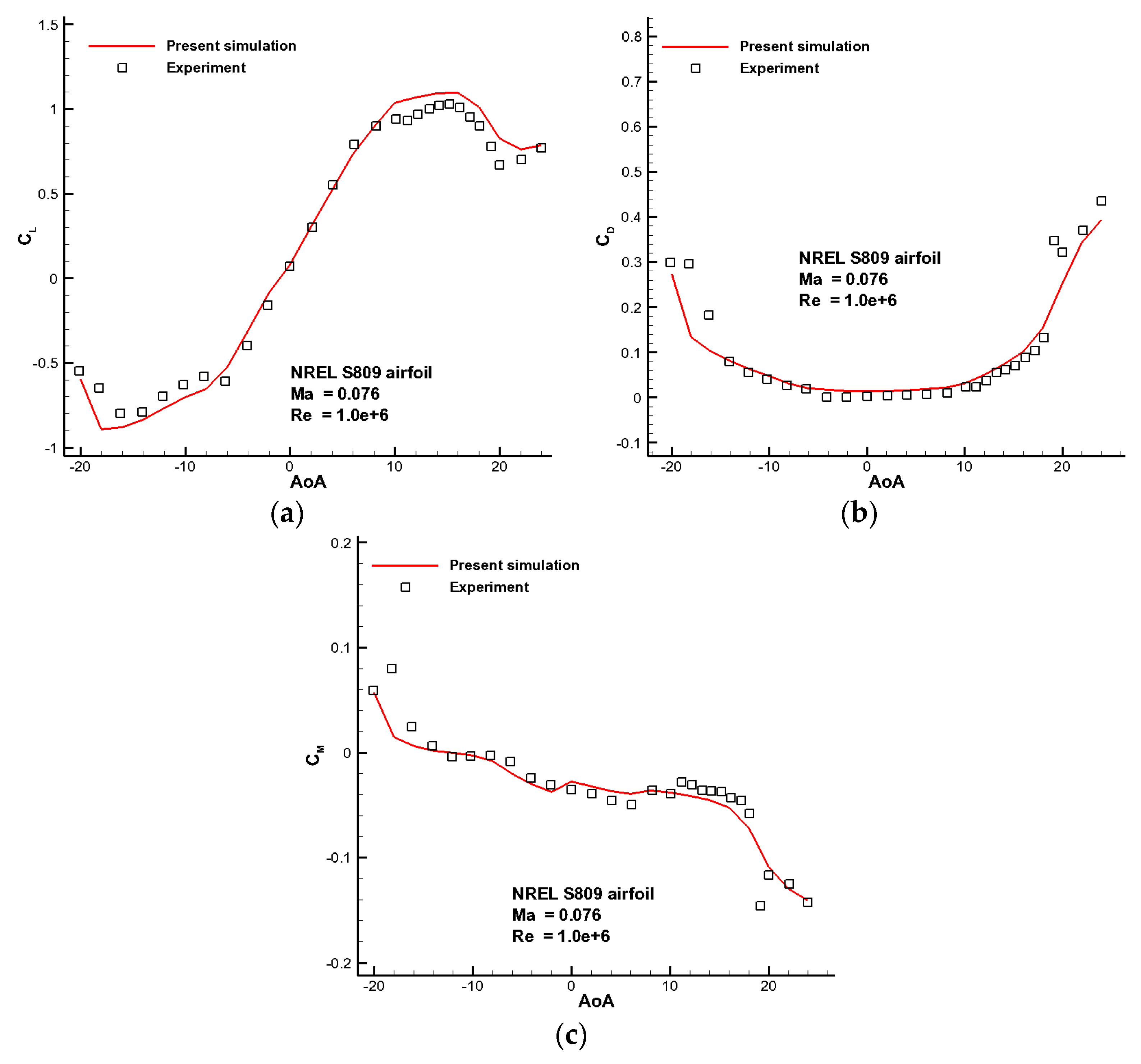
The medium mesh is further used to simulate a wide range of angles of attack from −20° to 24° for more validations. The computed aerodynamic force and moment coefficients are compared with experimental results in Figure 4. All the simulations are carried out at same Mach number 0.076 and Reynolds number 1.0 × 10⁶. The present static results will be used to compare with the next dynamic stall results which vary in a range of angles of attack between 4° and 24°. From Figure 4, for the range of angles of attack from −6° to 8°, the numerical results agree rather well with the measurement. After the flow separation occurrence, the lift is a little over-predicted but within an acceptable degree, and the variation trend is well captured. Overall, the present numerical results agree fairly well with experiment.

Figure 5 gives the comparison of surface pressure coefficient distributions with measurements for several AoA conditions, also showing rather good agreements except for large angles of attack over 20°.

4.1.2. Dynamic Characteristics and Time-Resolution Study

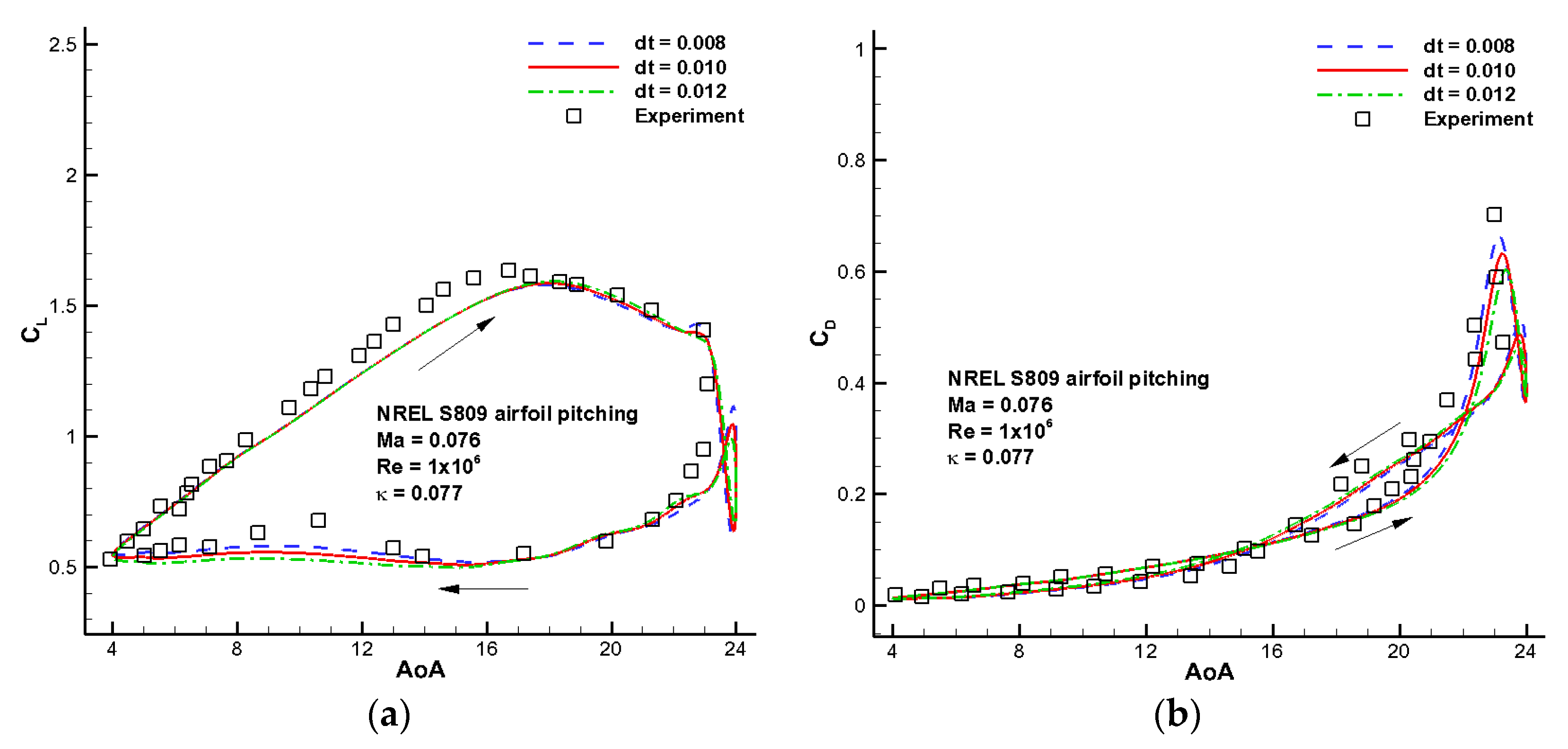
In the OSU experiment, unsteady data were obtained for the S809 airfoil model undergoing sinusoidal pitch oscillations with a comprehensive set of test conditions, including two angle of attack amplitudes, ±5.5° and ±10°; four Reynolds numbers, 0.75, 1.0, 1.25, and 1.4 million; three pitch oscillation reduced frequencies, 0.026, 0.052, and 0.077; and three mean angles of attack, 8°, 14°, and 20°. In the present study, the following conditions are selected for all of the validation simulations as well as the subsequent comparative studies: mean angle of attack α₀ = 14°, angle of attack amplitude α₁ = 10°, Reynolds number Re = 1.0 million, and reduced frequency κ = 0.077. The airfoil performs the sinusoidal pitch oscillation about its quarter chord point.

The simulations are performed using three different non-dimensional time steps (non-dimensionalized by c/V_∞) dt = 0.008, 0.010, 0.012, respectively, in order to investigate the time step sensitivity based on the aerodynamic coefficients. Four consecutive cycles are sufficient to obtain a periodic solution, and in the present study plotted curves are obtained from the fourth cycle. The comparison of numerical aerodynamic coefficients with experimental measurements are given in Figure 6, showing a reasonably good agreement. Hysteresis is present in the aerodynamic force coefficient curves as well as the moment coefficient curve. It is also shown that smaller time steps have little effects on the accuracy of the results, and hence the middle time step of dt = 0.010 is selected to carry out all the subsequent pitch oscillation cases for both the jet-off and jet-on configurations.

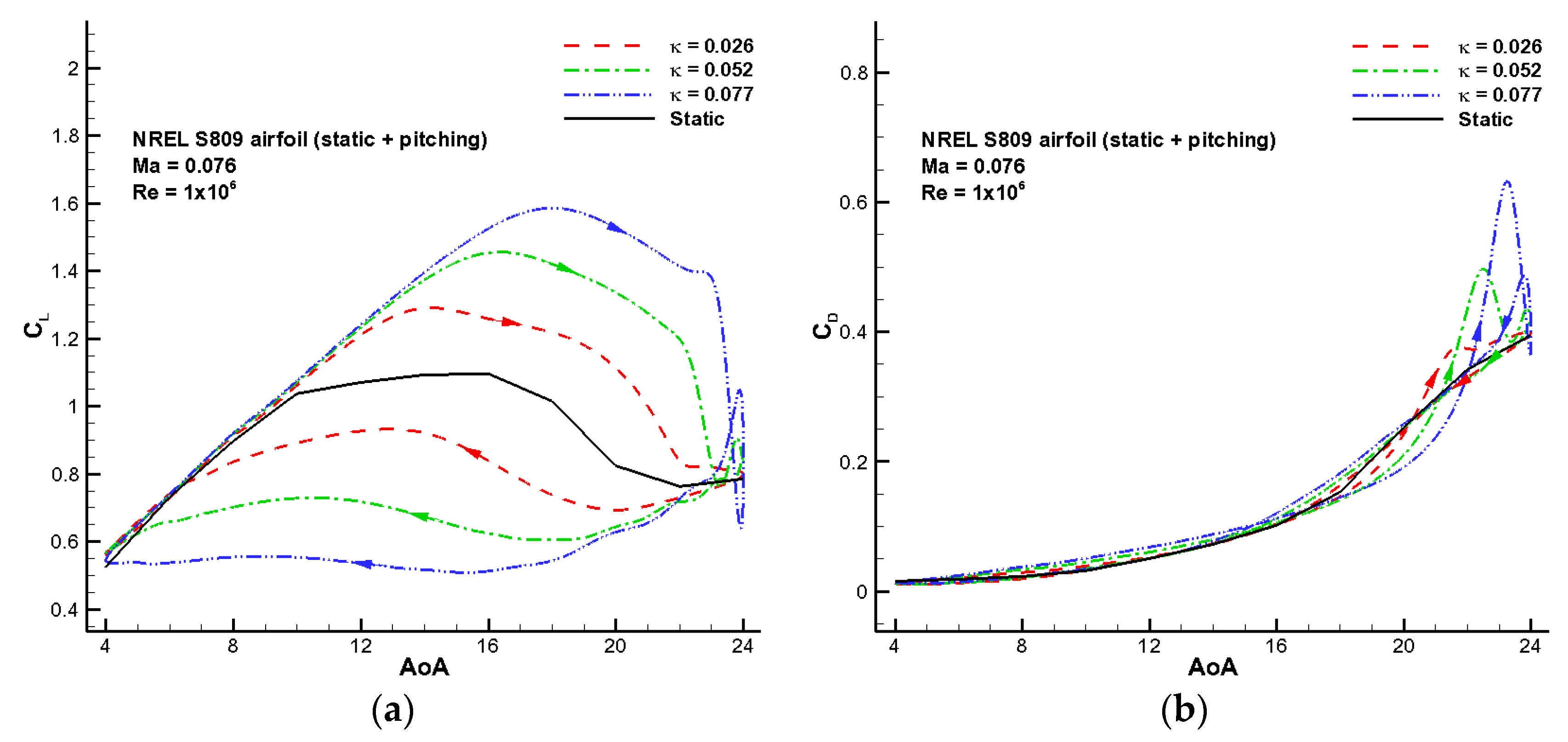
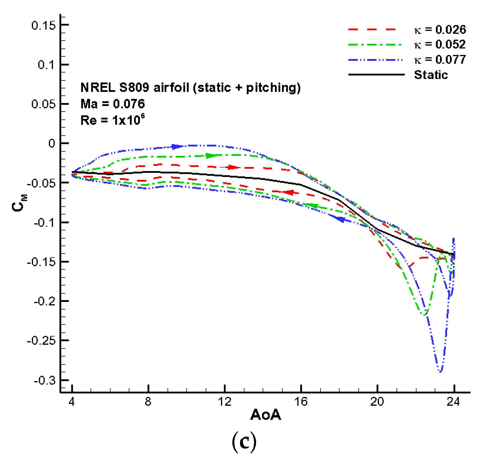
In Figure 7, the calculated results of both static and oscillating motions at three reduced frequencies 0.026, 0.052, 0.077 are plotted together, in order to clearly exhibit the effect of oscillating motion and reduced frequency on the airfoil aerodynamic performance. It can be found that the motion of airfoil and the parameter of reduced frequency have a substantial impact on the flow field. The oscillating motion leads to the appearance of hysteresis loops for all aerodynamic coefficients, and a larger reduced frequency leads to a larger opening in the hysteresis loops. The highest lift coefficient obtained during oscillation is correspondingly much higher than its static counterpart. The higher the reduced frequency, the higher the highest lift coefficient. It is also shown that a higher reduced frequency can generate even larger drag and moment peaks at high angles of attack, causing a greater extreme aerodynamic load which could lead to structural fatigue or even worse the total damage of the structure. One purpose of the present research is to reduce this kind of fluctuating extreme aerodynamic load by implementing a co-flow jet on the airfoil suction surface and will be presented later.

4.2. CFJ Simulation and Validation

A CFJ airfoil based on the NACA 6415 airfoil was tested by Dano et al. [17] in the University of Miami 24″×24″ wind tunnel facilities. The CFJ airfoil was a NACA 6415 with the injection and suction located at 7.5% and 88.5% of the chord, respectively. The injection and suction slot heights were 0.65% and 1.42% of the chord. In the experiment, the CFJ is provided by a separated high pressure source for the injection and a low pressure vacuum sink for the suction. The injection and suction flow conditions were independently controlled. A compressor supplied the injection flow and a vacuum pump generates the necessary low pressure for suction. Both mass flow rates in the injection and suction slots were measured using orifice mass flow meters. More experiment details can be found in [17]. The free stream Mach number was 0.03, and the chord-based Reynolds number was 195,000. The leading edge trip was used to achieve full turbulent boundary layer to be consistent with the CFD analysis. The open slot case in the experiment with momentum coefficient C_μ = 0.08 is chosen to validate the present solver for CFJ simulation.

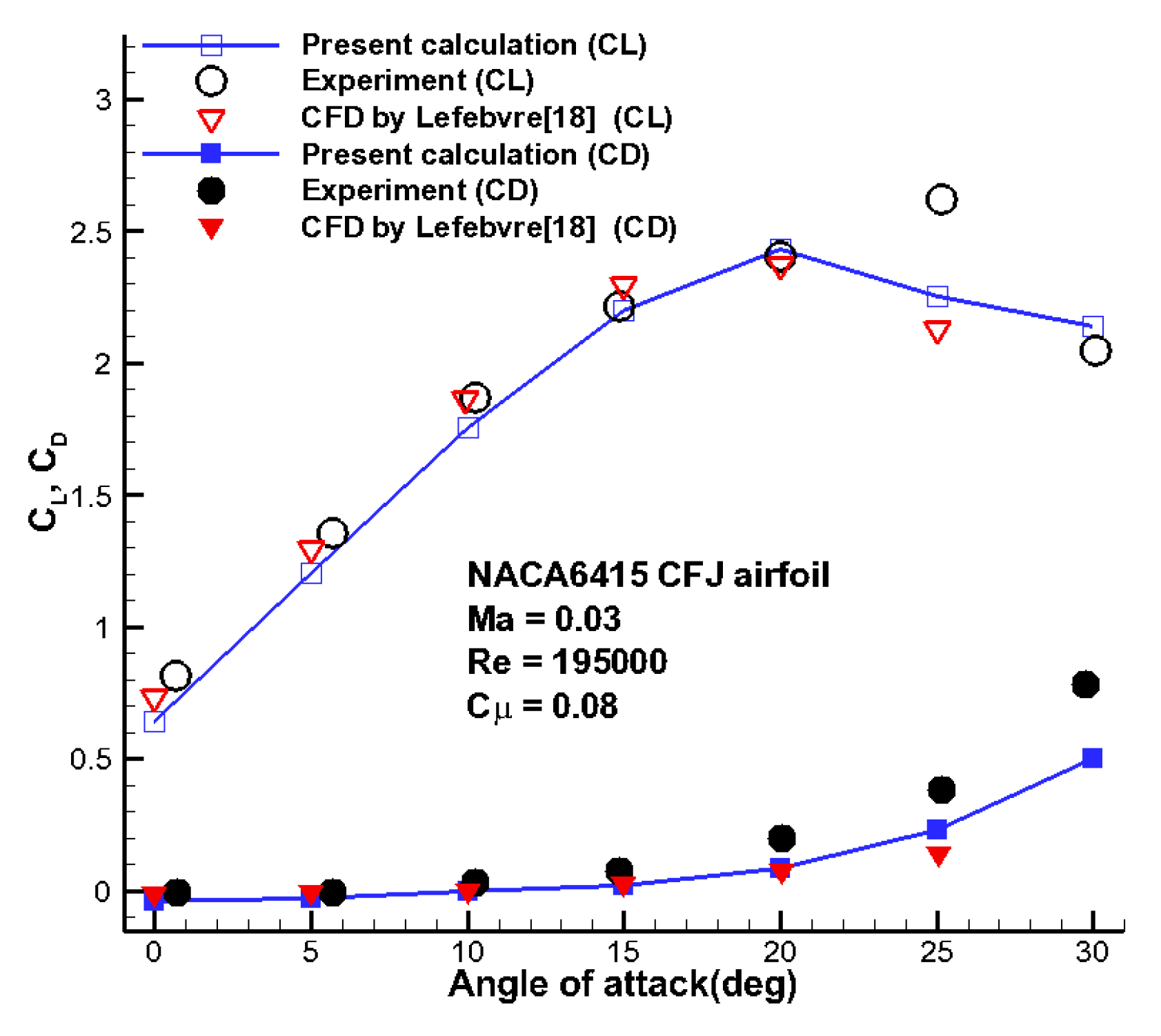
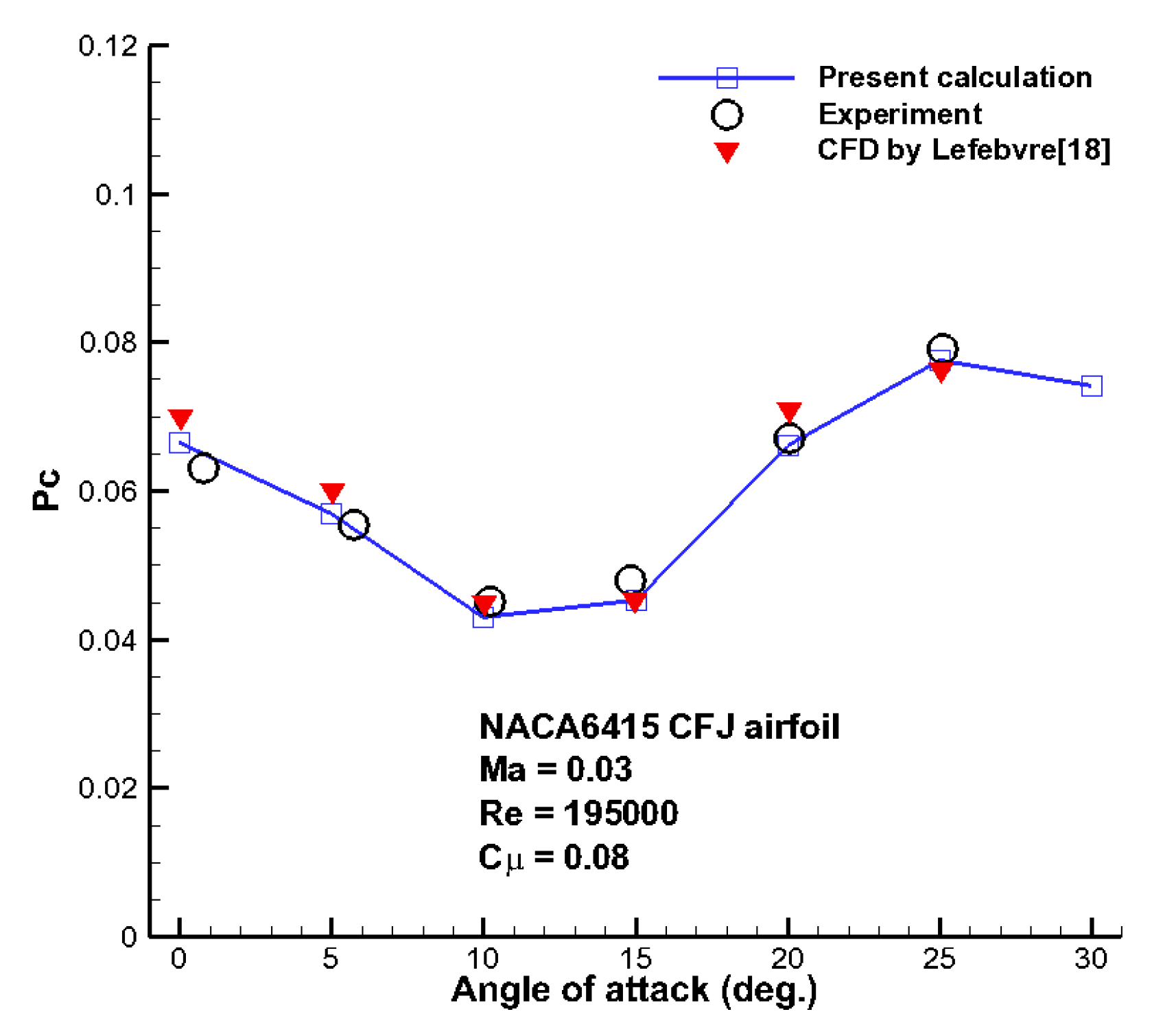
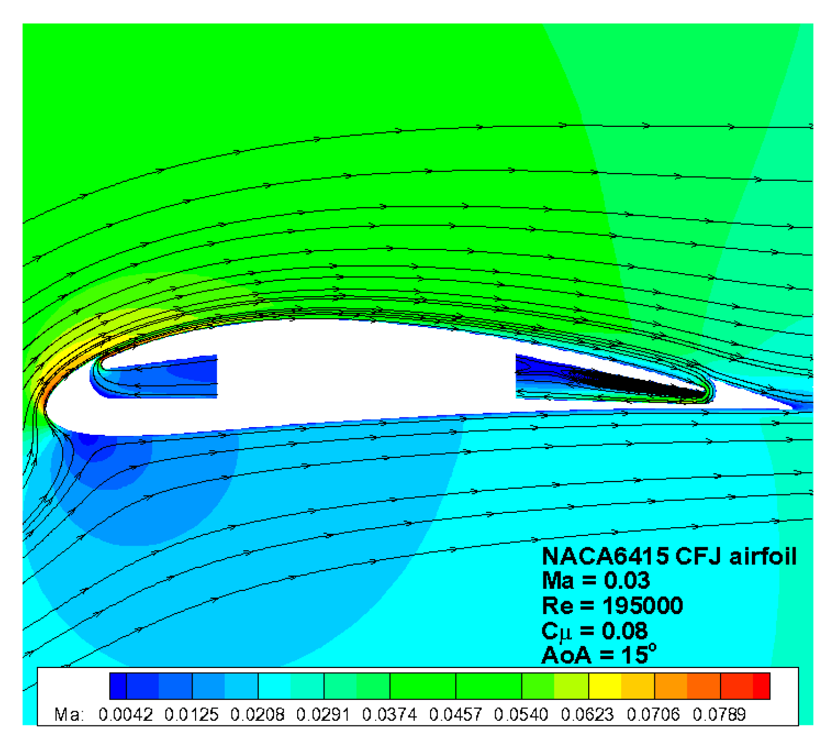
Based on the grid-resolution study in Section 4.1.1, the computational mesh for the present NACA 6415 CFJ airfoil is generated in a similar way according to the medium mesh for the NREL S809 CFJ airfoil. The computed lift, drag and power coefficients are presented in Figure 8 and Figure 9, and the flow field at AoA = 15° is shown in Figure 10. The present numerical results are compared with experimental as well as CFD results by Lefebvre et al. [18], showing fairly good agreements, especially for the power coefficient. For the lift coefficient, good agreement is achieved up to the highest AoA of 30°, except AoA of 25° where the lift is underpredicted by the present solver as well as Lefebvre et al. [18]. The computed drag coefficient is underpredicted when the AoA is greater than 15°. Among the comparisons, the computed power coefficient agrees the best with the experiment. The reason may be that the total pressure and total temperature are integrated parameters using mass average, which is easier to predict accurately than the drag that is determined by skin friction and pressure distribution. Overall, it is demonstrated that the present solver can predict the CFJ flow with a fairly good precision, and it is reliable to be used for the present numerical study of CFJ.

4.3. Inactive CFJ Cases

The co-flow jet flow control concept has a distinct feature with a jet channel on a large portion of the airfoil suction surface by a translation and slight rotation operation. This channel is necessary for the co-flow jet concept. However, the presence of a channel inevitably affects the original well-designed aerodynamic performance of the baseline airfoil when the co-flow jet is inactive, since it has changed the aerodynamic shape of the airfoil. The effect of the presence of a channel on the static characteristics of airfoil has been investigated in a previous work [21], showing that the channel will lead to a mild lift decrease, earlier stall, and drag increase. In the present study, the effect of a jet-off channel on the dynamic characteristics is studied by simulating the sinusoidal oscillation of the jet-off configuration at the same conditions as the baseline.

The numerical results are shown in Figure 11, and are compared with the baseline results. For the lift coefficient, the jet-off cases have an overall lower value than the baseline, especially in the range of lower angles of attack during down-stroke motion. In the upstroke process, the lift coefficient is constantly lower than the baseline till the angle of attack about 20°, after which the lift increases to a peak even larger than the corresponding baseline, and then experiences a rapid drop. This drastic variation consequently causes corresponding peaks in the drag coefficient and moment coefficient hysteresis loops. That is to say, with the jet-off channel, the wind turbine airfoil will experience a more severe extreme air load in terms of drag and moment.

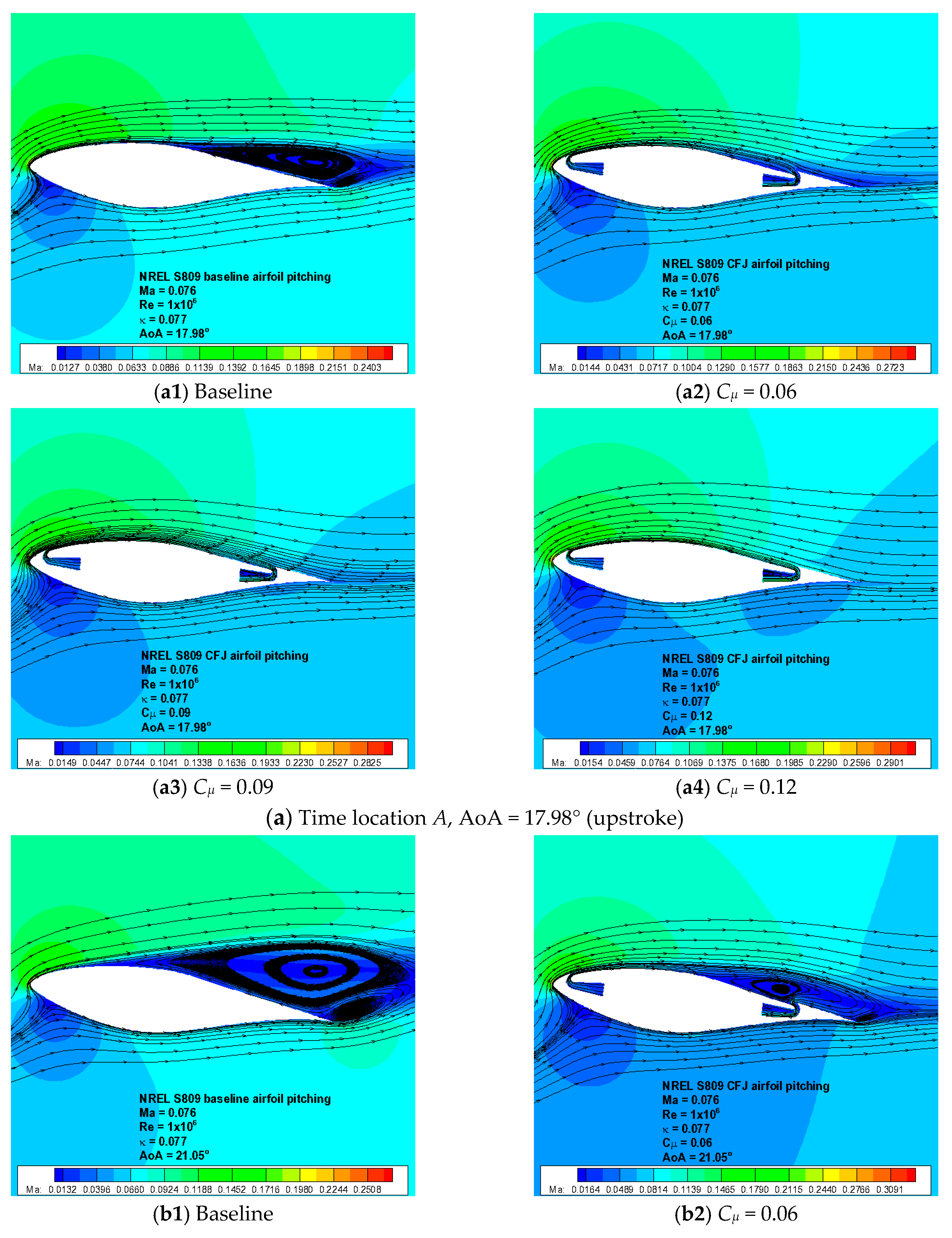
In the previous static study [21], the force and moment coefficient peaks in the jet-off case were not present, and hence it is expected to be the reflection of the pitch oscillation effect on the flow. To make clear the reason of the peak’s existence, the flow fields and pressure coefficient distributions of six specific time locations are plotted in Figure 12 and Figure 13, respectively. The six time locations are denoted by A, B, C, D, E, and F in Figure 11a, which cover the range of angles of attack that see the peak occurrence. For the purpose of comparison, the corresponding baseline flow fields and pressure coefficient distributions are also plotted in the same scale. At the time location A, the flow pattern of jet-off case is similar to the baseline, except that a small recirculating region exists behind the injection slot surface. It can be seen from the comparison of pressure coefficient distribution in Figure 13a that the presence of a channel results in a lower suction peak and a lower suction for a large proportion of the channel surface, causing the lift to decrease by a small amount, although the local suction is increased in the small recirculating region. Then the small standing vortex continues to increase in streamwise size as the angle of attack increases. At the time location B, the front vortex develops enough to connect with the trailing edge vortex. At the time location C, the front vortex and the trailing edge vortex start to combine together, causing the corresponding surface pressure lower than the baseline as shown in the comparison of pressure coefficient distribution in Figure 13c. At the time location D, the two vortices continue to merge, and the lift continues to increase. At time location E, the two vortices completely merge into one larger vortex, causing the lift to reach a maximum. By comparing the Mach contours in Figure 12i,j, it can be found that the flow velocity on the jet-off suction surface at the location about 70%c from the leading edge is much larger than that of baseline, causing much lower pressure. The difference between the pressures of this particular part of suction surface is evidently the reason that the forces and moment reach a peak. After the formation of a single larger vortex, the lift starts to decrease rapidly due to the convection of the vortex into the wake. At the time location F, the jet-off flow field presents a more complicated multiple-vortex feature, and the lift is lower than the baseline. Therefore, the dynamic process of vortex merging gives rise to the presence of peak which is a kind of extreme aerodynamic load.

4.4. Active CFJ Cases

As the main focus of present study, the dynamic characteristics of the S809 CFJ airfoil are investigated with three jet momentum coefficients C_μ = 0.06, 0.09, 0.12. Figure 14 shows comparison of unsteady aerodynamic characteristics between the baseline and CFJ cases with three momentum coefficients at Re = 1 × 10⁶. The overall lift coefficients of the CFJ cases are much higher than that of the baseline, while the drag and moment coefficients of the CFJ cases are much lower than that of the baseline. It is obvious for the CFJ cases that the co-flow jet with a higher momentum coefficient has a greater ability in the lift enhancement, and results in a wider range of the linear portion of the lift coefficient curves. With increasing momentum coefficient from 0.06 to 0.12, the aerodynamic coefficient loops exhibit smaller hysteresis as expected. A stronger jet can suppress the separation at higher angles of attack. It can be found in Figure 14a that for the CFJ case with C_μ = 0.06, at higher angles of attack larger than 21° and during the down-stroke, the lift coefficient curve presents a flow-separation characteristic, indicating that this C_μ level is not strong enough to suppress flow separation at angle of attack greater than 21°. However, for the case with C_μ = 0.12, the lift coefficient curve does not present a noticeable stall feature, demonstrating that a stronger jet can fully control the dynamic stall.

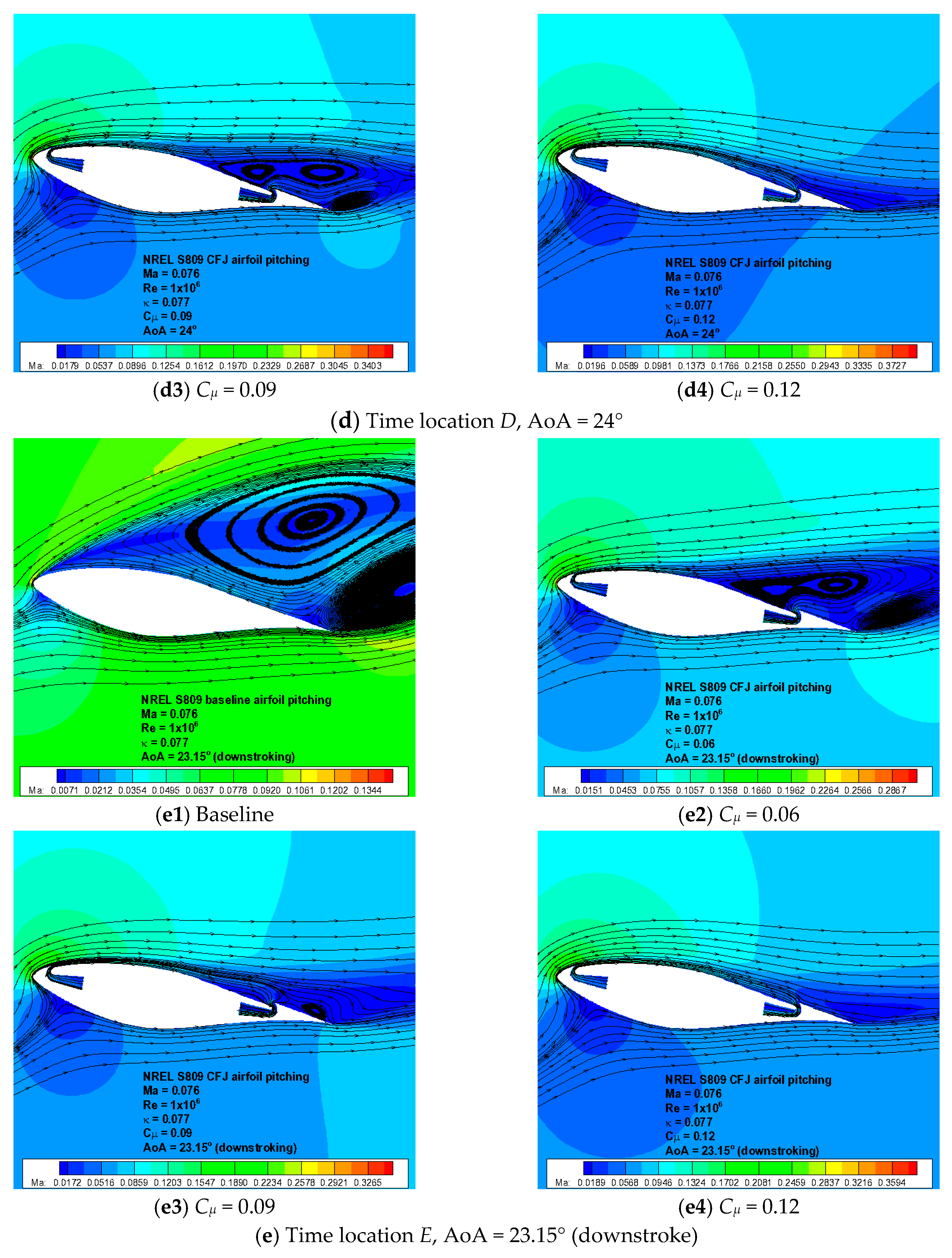
To show in detail and compare the abilities of co-flow jets with different C_μ levels in suppressing separation at large angles of attack, five typical instantaneous time locations for the case of κ = 0.077 are investigated in terms of flow field contours and streamlines as well as surface pressure coefficient distributions, as shown in Figure 15 and Figure 16. The five time locations are labeled in Figure 14a. The lift coefficients of time locations A, B, C are the highest values for the baseline, CFJ with C_μ = 0.06, CFJ with C_μ = 0.09, respectively. The angle of attack of the time location D is 24°, the maximum of the investigated pitch oscillation motion. The time location E is the position that it is most likely to occur a separation flow since it is the locally lowest point in the down-stroke hysteresis loop. All the four cases of baseline, C_μ = 0.06, 0.09, 0.12 are simultaneously investigated at each of the five time locations. In Figure 15a, it is shown that the baseline has a mild trailing edge separation, whereas the CFJ cases with all the three C_μ levels can completely suppress the separation. In Figure 15b, the baseline experiences a massive separation, and the CFJ with C_μ = 0.06 is not strong enough to suppress it. With stronger CFJ with C_μ = 0.09 and 0.12, this massive separation can still be completely suppressed. In Figure 15c, a stronger separation exists in the baseline case as well as the CFJ case with C_μ = 0.06 due to the large angle of attack being 22.77°. But with a stronger CFJ with C_μ = 0.09 and 0.12, the separation still disappears. In Figure 15d, at the highest angle of attack in the pitch motion, the baseline, CFJ with C_μ = 0.06 and 0.09 are all undergoing a separation, while the CFJ with C_μ = 0.12 remains the ability of completely suppressing separation. At the down-stroke time location E, the flow field with CFJ C_μ = 0.12 remains attached, demonstrating a perfect performance of CFJ in suppressing dynamic stall.

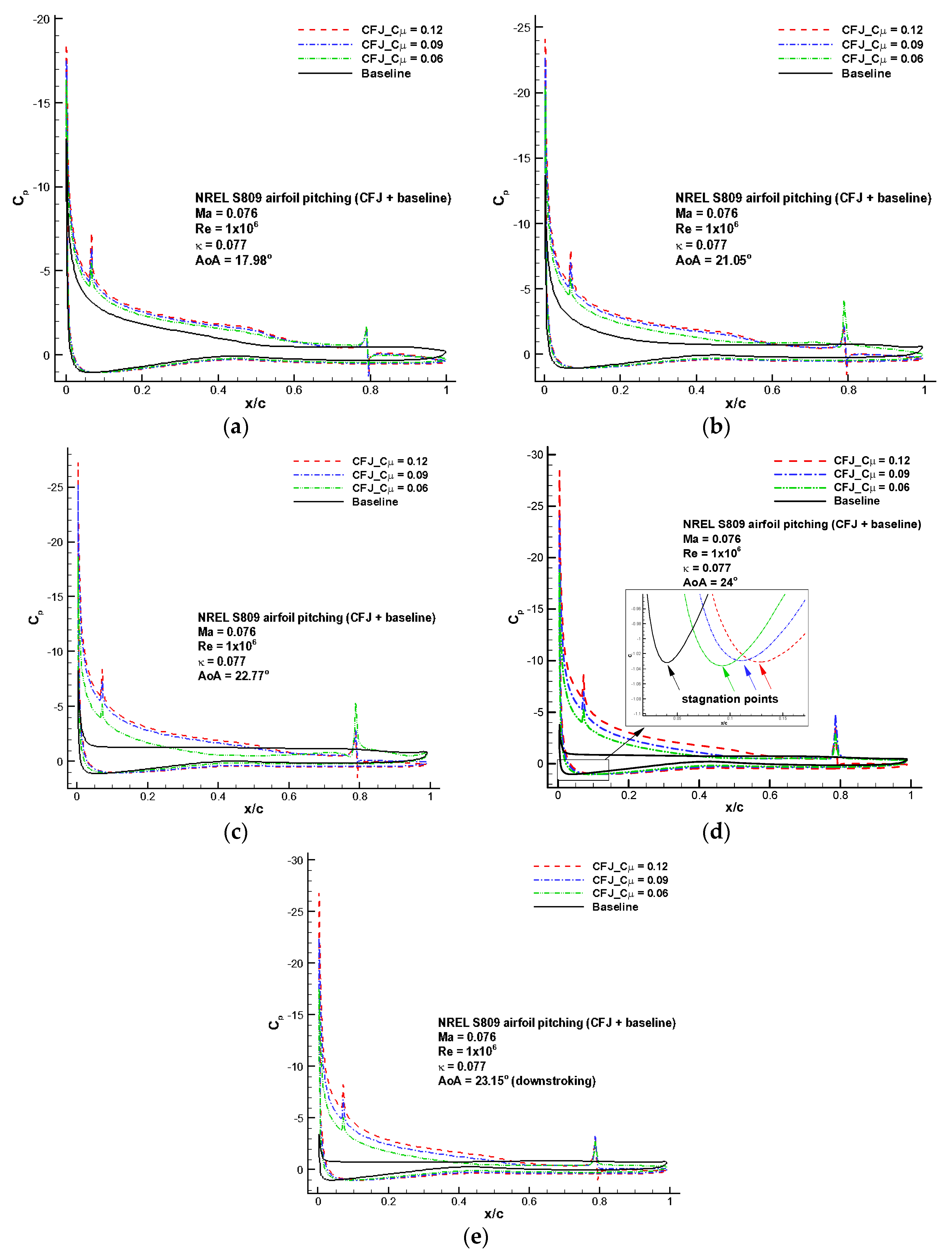
Figure 16 presents the corresponding pressure coefficient distributions for the five time locations, showing that enclosed area is larger for the cases with a higher jet momentum coefficient, representing a higher lift. From the view of the Kutta-Joukowski theorem [35], a higher lift corresponds to a larger circulation, which is embodied in how far downstream the location of stagnation point is.

The time location D is chosen to show this interesting phenomenon in Figure 16d, which in the enlarged window shows that the CFJ case with the highest C_μ = 0.12 has the most downstream stagnation point while the baseline has the most front stagnation point.

One purpose of the present study is to find out the performance of the CFJ in reducing the fluctuating extreme loads, especially the pitching drag force and moment.

Table 3. Comparison of amplitudes of force and moment coefficients (κ = 0.077).

Coefficient	Baseline	Cμ = 0.06	Cμ = 0.09	Cμ = 0.12
CL,min	0.5083	0.7469	0.8022	0.8389
CL,max	1.5862	2.0902	2.2719	2.4680
CL,amp	1.0779	1.3433	1.4697	1.6291
ΔCL,amp	–	24.62%↑	36.35%↑	51.14%↑
CD,min	0.0121	−0.0184	−0.0398	−0.0583
CD,max	0.6323	0.1708	0.0922	0.0781
CD,amp	0.6202	0.1892	0.1320	0.1364
ΔCD,amp	–	69.49%↓	78.72%↓	78.01%↓
CM,min	−0.2899	−0.2090	−0.1281	−0.1361s
CM,max	−0.0027	−0.0381	−0.0596	−0.0688
CM,amp	0.2872	0.1709	0.0685	0.0673
ΔCM,amp	–	40.49%↓	76.15%↓	76.57%↓

presents the amplitudes of the aerodynamic hysteresis loops for all cases with three different jet momentum coefficients, as well as the variation quantities of the amplitudes of the CFJ cases relative to those of the baseline. It is shown that the amplitude of lift coefficient can be significantly increased by implementing CFJ, while the amplitudes of drag and moment coefficients can be significantly reduced. The enhanced lift is beneficial for power generation, while the reduction of drag and moment is beneficial to the structural fatigue problem. The amplitude of lift can be enhanced by up to 51.14% in the CFJ case with C_μ = 0.12, the amplitude of drag can be reduced by as much as 78.72% with C_μ = 0.09, and the amplitude of moment can be reduced by 76.57% with C_μ = 0.12, as shown in Table 3. It should also be noted that in terms of drag and moment reduction, the CFJ with C_μ = 0.09 and 0.12 have an equivalent ability, meaning that a stronger jet with C_μ larger than 0.09 cannot necessarily result in a better performance in further reducing the amplitudes of drag and moment coefficients, although it may bring a further enhancement in lift. The amount of moment amplitude reduction only increases from 76.15% to 76.57% when C_μ varies from 0.09 to 0.12, and the amount of drag amplitude reduction even decreases from 78.72% to 78.01%. Overall, the study exhibits a rather encouraging and desired result: the CFJ concept can greatly enhance the lift, reduce the fluctuating drag and moment, leading to a larger output of wind energy, while reducing the potential structural fatigue damage.

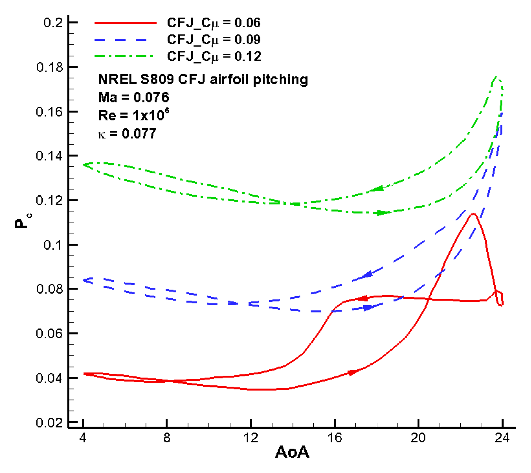
4.5. Energy Consumption Analysis

The consideration of energy cost of a flow control method is important in the all-round assessment of the method’s practicability and economy. As an active flow control method, the CFJ implementation needs a certain amount of energy input to perform its effect on the flow field.

Figure 17 gives the comparison of power coefficient hysteresis loops for all three C_μ levels, showing that more power input is required to pressurize the jet flow for a higher C_μ level jet. In the attached flow regime, the required power input decreases as the angle of attack increases. The reason is, from the view of airfoil aerodynamics, the pressure in the vicinity of the injection slot which is near the leading edge becomes lower when angle of attack increases, namely the suction peak becomes gradually higher with increasing angle of attack before the flow separates. The low pressure will benefit the power consumption, because the pump will perform less work to drive the jet flow. On the other hand, the pressure around the suction slot which is near the trailing edge is relatively higher due to the pressure recovery process on the airfoil suction surface. This higher pressure also makes it easier for the pump to suck flow from the suction slot. The combination of injection and suction takes full advantage of the pressure difference between the injection and suction slots, and hence results in relatively lower energy consumption. At very high angles of attack, the energy input increases with increasing angle of attack, regardless the flow is attached or separated. For the separated flow at the high angles of attack in the case with C_μ = 0.06, the energy input reaches a peak during the upstroke process, while keeps at a nearly constant high level during the down-stroke process. Even so, the cycle averaged value of energy input of the case with C_μ = 0.06 is still much lower than that of cases with higher C_μ levels, which will be seen in

Table 4. Averaged aerodynamic and power coefficients in one oscillation cycle (κ = 0.077).

Coefficient	Baseline	Cμ = 0.06	Cμ = 0.09	Cμ = 0.12
CL,ave	0.8615	1.3313	1.5695	1.7090
CD,ave	0.1625	0.0424	0.0189	0.0052
CM,ave	−0.0801	−0.0932	−0.0947	−0.1011
Pc,ave	–	0.0558	0.0916	0.1325

.

The analysis of energy consumption performance of the present two-dimensional CFJ implementation is given here based on an average estimation, and more comprehensive computation and analysis are left to be conducted in further three-dimensional wind turbine rotor simulation work. Table 4 gives the time-averaged aerodynamic and power coefficients, which are calculated from one oscillation cycle. It is shown that the lift and power increase with C_μ, while drag and moment decrease with C_μ. The reduction of drag with increasing C_μ is attributed to the contribution of jet reaction force. Indeed, the energy consumed by the pump is partly injected into the main flow and energizes the main flow as well as the boundary layer, resulting in a reduced drag.

For simplicity, assume that the free stream flow direction is perpendicular to the rotor plane with a magnitude of $V_{\infty }/\sqrt{2}$ (V_∞ is the local coming flow seen by the sectional airfoil, which is equal to 0.076 × 340 m/s = 25.84 m/s). Assume that the controlled S809 airfoil is located at a position that rotates at a speed equal to the free stream velocity. Hence, a decomposed component of airfoil lift by multiplying the total lift with $\sqrt{2}/2$ will contribute to the energy generation. Assume that the wind turbine efficiency of energy generation from the torque is η_e = 0.85. Then the coefficient of rotor power generation P_e by 2-D airfoil with unit span can be calculated by:

$$P_{e,ave}=\frac{LV}{q_{\infty }{V}_{\infty }}\cdot {\eta }_e=\frac{0.5{\rho }_{\infty }{V}_{\infty }^{2}c(1)\sqrt{2}/2C_{L,ave}\cdot V_{\infty }/\sqrt{2}}{0.5{\rho }_{\infty }{V}_{\infty }^{3}c(1)}\cdot {\eta }_e=\frac{1}{2}{\eta }_e{C}_{L,ave}$$

(5)

The power loss for pumping can be calculated in percentage of baseline rotor power by

$$P_{pumping,ave}=\frac{P_{c,ave}}{P_{e,ave,baseline}}\times 100\%$$

(6)

The power gain through increased C_L,ave can be calculated by

$$P_{gain,ave}=\frac{\Delta L\cdot V}{q_{\infty }{V}_{\infty }}\cdot {\eta }_e/P_{e,ave,baseline}\times 100\%=\frac{\Delta C_{L,ave}}{C_{L,ave,baseline}}\times 100\%$$

(7)

Table 5. Power performance analysis for different C_μ levels (κ = 0.077).

Cases	Ppumping	Pgain	Pgain − Ppumping
Cμ = 0.06	15.24%	54.53%	39.29%
Cμ = 0.09	25.02%	82.18%	57.16%
Cμ = 0.12	36.19%	98.37%	62.18%

shows the power performance analyses for different C_μ levels. It is shown that more power can be gained by using larger jet strength. However, it should be noted that the increase of net power gain from C_μ = 0.09 to C_μ = 0.12 is much lower than that from C_μ = 0.06 to C_μ = 0.09, implying that a too strong jet will not necessarily have a better performance, and there is an optimal jet strength choice.

5. Conclusions

Dynamic stall control using a co-flow jet is systematically investigated by numerically solving the unsteady Reynolds-Averaged Navier-Stokes equations. The solver is validated by comparing the numerical results with a baseline experiment and a CFJ experiment. The jet-off configuration is simulated to assess the negative effect of the jet channel existence. The dynamic stall control performance of the CFJ is investigated by implementing co-flow jets at three momentum coefficients on the pitching CFJ airfoil and comparing results with the baseline. The detailed instantaneous flow field contours and streamlines, and surface pressure coefficient distributions are examined and analyzed. The energy consumption of applying a co-flow jet is computed and analyzed to assess the CFJ concept. The conclusions obtained are as follows:

(1)

The solver can predict well the aerodynamic characteristics of the baseline airfoil as well as the CFJ airfoil, including the static characteristics and dynamic pitch oscillation characteristics on the basis of grid-resolution and time-step resolution studies.

(2)

When the co-flow jet is inactive, the jet channel has a negative effect on the airfoil dynamic aerodynamic performance. The lift is reduced, while the drag and moment increase. In particular, the drag and moment hysteresis loops exhibit a higher local peak which, as a form of fluctuating extreme aerodynamic loads on the structure, can cause potential structural fatigue damage.

(3)

A co-flow jet can effectively suppress dynamic stall, especially with a higher momentum coefficient level which can fully control the separation. The amplitude of lift increases and it is beneficial to the energy output. The amplitudes of drag and moment are significantly reduced, showing an attractive performance in reducing the fluctuating aerodynamic loads on the wind turbine structure. The dynamic stall caused by unsteady inflow due to atmospheric turbulence or wakes form other turbines in a wind farm can lead to generation of unsteady torque at the shaft. By applying the CFJ concept, it is expected that the unsteady torque at the shaft can be greatly mitigated.

(4)

The co-flow jet concept makes use of the advantageous pressure difference between injection and suction slots, and requires a minimum energy input to pump the jet. A positive net power gain is obtained by the approximate two-dimensional energy consumption analysis. It is demonstrated that the CFJ method is an applicable and economic approach in dynamic stall control.

Numerical results of the present study show a powerful ability for the CFJ to suppress dynamic stall, theoretically proving it’s promising application for wind turbines. However, it should be noted that the implementation of a CFJ will give rise to some concerns, including added weight, complexity of spanwise slots, control of recirculating jets and potential extra maintenance. The extra maintenance is an important issue for the long-term cost analysis, and the potential situation in which the co-flow jet is closed due to failure of the device should be taken into account. From the studies shown in this paper, the co-flow jet channel has a moderate negative effect on the aerodynamic performance when the device doesn’t work. In view of the long-term benefit from the CFJ application, it is worthwhile to make efforts to reduce the maintenance and keep carrying this research further. In fact, the fast development of material science and manufacturing technology have made great contributions in reducing rotor weight, allowing more complicated designs and enhancing structural reliability. In practice, the high-pressure and low-pressure cavities could be connected by a pump inside the blade or by pipes linked to special pressurization equipment integrated in the stationary part of the wind turbine system. For large scale wind turbines, the chord length and sectional airfoil thickness near the blade root are relatively large and the inflow velocity is relatively low, making it feasible to install a pump inside the blade. The slots and channel could be designed as a continuous whole or be discretely distributed on the blade surface. Three-dimensional simulations would be helpful to understand more about the flow phenomena and mechanism of the CFJ concept, which is our future work plan.

References

1. Tchakoua, P.; Wamkeue, R.; Ouhrouche, M.; Slaoui-Hasnaoui, F.; Tameghe, T.A.; Ekemb, G. Wind turbine condition monitoring: State-of-the-art review, new trends, and future challenges. Energies 2014, 7, 2595–2630. [Google Scholar]
2. World Wind Energy Association. Half Year Report. 2014. Available online: http://www.wwindea.org/webimages/WWEA_half_year_report_2014.pdf (accessed on 6 August 2015).
3. Mo, W.; Li, D.; Wang, X.; Zhong, C. Aeroelastic coupling analysis of the flexible blade of a wind turbine. Energy 2015, 89, 1001–1009. [Google Scholar] [CrossRef]
4. Sanaye, S.; Hassanzadeh, A. Multi-objective optimization of airfoil shape for efficiency improvement and noise reduction in small wind turbines. J. Renew. Sustain. Energy 2014, 6, 053105. [Google Scholar] [CrossRef]
5. Lee, J.W.; Kim, J.K.; Shin, H.K.; Bang, H.J. Active load control for wind turbine blades using trailing edge flap. Wind Struct. 2013, 16, 263–278. [Google Scholar] [CrossRef]
6. Macquart, T.; Maheri, A.; Busawon, K. Microtab dynamic modeling for wind turbine blade load rejection. Renew. Energy 2014, 64, 144–152. [Google Scholar] [CrossRef]
7. Johnson, S.J.; Baker, J.P.; van Dam, C.P.; Berg, D. An overview of active load control techniques for wind turbines with an emphasis on microtabs. Wind Energy 2010, 13, 239–253. [Google Scholar] [CrossRef]
8. Gao, L.Y.; Zhang, H.; Liu, Y.Q.; Han, S. Effects of vortex generators on a blunt trailing-edge airfoil for wind turbines. Renew. Energy 2015, 76, 303–311. [Google Scholar] [CrossRef]
9. Wang, G.N.; Lewalle, J.; Glauser, M.; Walczak, J. Investigation of benefits of unsteady blowing actuation on a 2D wind turbine blade. J. Turbul. 2013, 14, 165–189. [Google Scholar] [CrossRef]
10. Müller-Vahl, H.F.; Strangfeld, C.; Nayeri, C.; Paschereit, C.; Greenblatt, D. Thick Airfoil Deep Dynamic Stall and Its Control. Available online: http://arc.aiaa.org/doi/10.2514/6.2013-854 (accessed on 22 December 2015).
11. Tongchitpakdee, C.; Benjanirat, S.; Sankar, L.N. Numerical Studies of the Effects of Active and Passive Circulation Enhancement Concepts on Wind Turbine Performance. J. Sol. Energy Eng. 2006, 128, 432–444. [Google Scholar] [CrossRef]
12. Yen, J.; Ahmed, N.A. Enhancing vertical axis wind turbine by dynamic stall control using synthetic jets. J. Wind Eng. Ind. Aerodyn. 2013, 114, 12–17. [Google Scholar] [CrossRef]
13. Greenblatt, D.; Ben-Harav, A.; Mueller-Vahl, H. Dynamic stall control on a vertical-axis wind turbine using plasma actuators. AIAA J. 2014, 52, 456–462. [Google Scholar] [CrossRef]
14. Zha, G.C.; Carroll, B.; Paxton, C.; Conley, C.A.; Wells, A. High performance airfoil with co-flow jet flow control. AIAA J. 2007, 45, 2087–2090. [Google Scholar] [CrossRef]
15. Zha, G.C.; Gao, W.; Paxton, C.D. Jet effects on co-flow jet airfoil performance. AIAA J. 2007, 45, 1222–1231. [Google Scholar] [CrossRef]
16. Wang, B.Y.; Haddoukessouni, B.; Levy, J.; Zha, G.C. Numerical investigations of injection slot size effect on the performance of co-flow jet airfoil. J. Aircr. 2008, 45, 2084–2091. [Google Scholar] [CrossRef]
17. Dano, B.P.E.; Zha, G.C.; Castillo, M. Experimental study of co-flow jet airfoil performance enhancement using discrete jets. In Proceedings of the 49th AIAA Aerospace Sciences Meeting including the New Horizons Forum and Aerospace Exposition, Orlando, FL, USA, 4–7 January 2011.
18. Lefebvre, A.; Dano, B.P.E.; Fronzo, M.D.; Bartow, W.B.; Zha, G.C. Performance of co-flow jet airfoil with variation of Mach number. In Proceedings of the 51st AIAA Aerospace Sciences Meeting including the New Horizons Forum and Aerospace Exposition, Grapevine, TX, USA, 7–10 January 2013.
19. Lefebvre, A.; Zha, G.C. Pitching airfoil performance enhancement using co-flow jet control at high Mach number. In Proceedings of the 52nd Aerospace Sciences Meeting, National Harbor, MD, USA, 13–17 January 2014.
20. Im, H.S.; Zha, G.C.; Dano, B. Large eddy simulation of co-flow jet airfoil at high angle of attack. J. Fluids Eng. 2014, 136, 02110. [Google Scholar]
21. Xu, H.Y.; Xing, S.L.; Ye, Z.Y. Numerical study of the S809 airfoil aerodynamic performance using a co-flow jet active control concept. J. Renew. Sustain. Energy 2015, 7, 023131. [Google Scholar] [CrossRef]
22. Reuss, R.R.; Hoffmann, M.J.; Gregorek, G.M. Effects of Grit Roughness and Pitch Oscillations on the S809 Airfoil; Technical Report NREL/TP-442-7817; National Renewable Energy Laboratory (NREL): Fort Collins, CO, USA, 1995. [Google Scholar]
23. Jameson, A. Time dependent calculations using multi-grid with applications to unsteady flows past airfoils and wings. In Proceedings of the 10th Computational Fluid Dynamics Conference, Honolulu, HI, USA, 24–27 June 1991.
24. Yoon, S.; Jameson, A. Lower-Upper Symmetric-Gauss-Seidel Method for the Euler and Navier-Stokes Equations. AIAA J. 1988, 26, 1025–1026. [Google Scholar] [CrossRef]
25. Roe, P. Approximate Riemann solvers, parameter vectors, and difference schemes. J. Comput. Phys. 1981, 43, 357–372. [Google Scholar] [CrossRef]
26. Van Leer, B. Towards the ultimate conservative difference scheme, V: A second order sequel to Godunov’s method. J. Comput. Phys. 1979, 32, 101–136. [Google Scholar] [CrossRef]
27. Hermanns, M. Parallel Programming in FORTRAN 95 Using OpenMP; Technical Report. Universidad Politecnica De Madrid: Madrid, Spain, 2002. Available online: http://www.openmp.org/presentations/miguel/F95_OpenMPv1_v2.pdf (accessed on 25 October 2015).
28. Xu, H.Y.; Xing, S.L.; Ye, Z.Y. Investigation on the unstructured rotational dynamic overset grids. Aircr. Eng. Aerosp. Technol. 2015, 87, 293–304. [Google Scholar] [CrossRef]
29. Xu, H.Y.; Ye, Z.Y.; Shi, A.M. Numerical study of propeller slipstream based on unstructured dynamic overset grids. J. Aircr. 2012, 49, 384–389. [Google Scholar] [CrossRef]
30. Xu, H.Y.; Ye, Z.Y. Euler calculation of rotor-airframe interaction based on unstructured overset grids. J. Aircr. 2011, 48, 707–712. [Google Scholar] [CrossRef]
31. Xu, H.Y.; Ye, Z.Y. Coaxial rotor helicopter in hover based on unstructured dynamic overset grids. J. Aircr. 2010, 47, 1820–1824. [Google Scholar] [CrossRef]
32. Xu, H.Y.; Xing, S.L.; Ye, Z.Y. Numerical study of an airfoil/rotating-slotted-cylinder based flutter exciter. J. Aircr. 2015, 52, 2100–2105. [Google Scholar] [CrossRef]
33. Xu, H.Y.; Ye, Z.Y. Numerical simulation of rotor-airframe aerodynamic interaction based on unstructured dynamic overset grids. Sci. China Technol. Sci. 2012, 55, 2798–2807. [Google Scholar] [CrossRef]
34. Somers, D.M. Design and Experimental Results for the S809 Airfoil; Report No. NREL/SR-440-6918; National Renewable Energy Laboratory: Fort Collins, CO, USA, 1997. [Google Scholar]
35. Anderson, J.D., Jr. Fundamentals of Aerodynamics, 5th ed.; McGraw-Hill: New York, NY, USA, 2011. [Google Scholar]
Figure 1. Co-flow jet conceptual airfoil.
Energies 09 00429 g001
Figure 2. The computational models of S809 CFJ airfoil: (a) Jet-on; (b) Jet-off.
Energies 09 00429 g002
Figure 3. O-mesh for S809 airfoil (medium level).
Energies 09 00429 g003
Figure 4. Comparisons of computed static aerodynamic coefficients with experiment: (a) Lift coefficient; (b) Drag coefficient; (c) Moment coefficient.
Energies 09 00429 g004
Figure 5. Comparisons of surface pressure coefficient distributions with experiment: (a) AoA = 6.1°; (b) AoA = 12.2°; (c) AoA = 18.1°; (d) AoA = 24°.
Energies 09 00429 g005aEnergies 09 00429 g005b
Figure 6. Comparison of aerodynamic coefficient loops for reduced frequency κ = 0.077: (a) Lift coefficient; (b) Drag coefficient; (c) Moment coefficient.
Energies 09 00429 g006aEnergies 09 00429 g006b
Figure 7. Comparison of aerodynamic coefficient loops for the static and oscillating motions under three reduced frequencies: (a) Lift coefficient; (b) Drag coefficient; (c) Moment coefficient.
Energies 09 00429 g007aEnergies 09 00429 g007b
Figure 8. Comparison of lift and drag coefficients between experiment and CFD simulations.
Energies 09 00429 g008
Figure 9. Comparison of power coefficient between experiment and CFD simulations.
Energies 09 00429 g009
Figure 10. Streamlines and Mach contour at AoA 15°.
Energies 09 00429 g010
Figure 11. Comparison of aerodynamic coefficient loops for reduced frequency κ = 0.077: (a) Lift coefficient; (b) Drag coefficient; (c) Moment coefficient.
Energies 09 00429 g011
Figure 12. Comparison of flow fields for six instantaneous angles of attack: (a) Time location A for jet-off case; (b) Time location A for baseline case; (c) Time location B for jet-off case; (d) Time location B for baseline case; (e) Time location C for jet-off case; (f) Time location C for baseline case; (g) Time location D for jet-off case; (h) Time location D for baseline case; (i) Time location E for jet-off case; (j) Time location E for baseline case; (k) Time location F for jet-off case; (l) Time location F for baseline case.
Energies 09 00429 g012aEnergies 09 00429 g012b
Figure 13. Comparisons of pressure coefficient distributions for six instantaneous angles of attack: (a) Time location A; (b) Time location B; (c) Time location C; (d) Time location D; (e) Time location E; (f) Time location F.
Energies 09 00429 g013
Figure 14. Comparison of aerodynamic coefficient loops for reduced frequency κ = 0.077: (a) Lift coefficient; (b) Drag coefficient; (c) Moment coefficient.
Energies 09 00429 g014
Figure 15. Comparison of flow fields at five instantaneous angles of attack for reduced frequency κ = 0.077. (a) Time location A, AoA = 17.98° (upstroke); (a1) Baseline; (a2) Cμ = 0.06; (a3) Cμ = 0.09; (a4) Cμ = 0.12; (b) Time location B, AoA = 21.05° (upstroke); (b1) Baseline; (b2) Cμ = 0.06; (b3) Cμ = 0.09; (b4) Cμ = 0.12; (c) Time location C, AoA = 22.77° (upstroke); (c1) Baseline; (c2) Cμ = 0.06; (c3) Cμ = 0.09; (c4) Cμ = 0.12; (d) Time location D, AoA = 24°; (d1) Baseline; (d2) Cμ = 0.06; (d3) Cμ = 0.09; (d4) Cμ = 0.12; (e) Time location E, AoA = 23.15° (downstroke); (e1) Baseline; (e2) Cμ = 0.06; (e3) Cμ = 0.09; (e4) Cμ = 0.12.
Energies 09 00429 g015aEnergies 09 00429 g015bEnergies 09 00429 g015c
Figure 16. Comparison of pressure coefficient distributions at five instantaneous angles of attack: (a) Time location A, AoA = 17.98° (upstroke); (b) Time location B, AoA = 21.05° (upstroke); (c) Time location C, AoA = 22.77° (upstroke); (d) Time location D, AoA = 24°; (e) Time location E, AoA = 23.15° (downstroke).
Energies 09 00429 g016
Figure 17. Comparison of the power coefficients between different Cμ levels.
Energies 09 00429 g017